
Parametric Optimization of Thin-Walled 3D Beams with Perforation Based on Homogenization and Soft Computing


Abstract
:1. Introduction
2. Materials and Methods
2.1. Study Objective and Optimization Frameworks
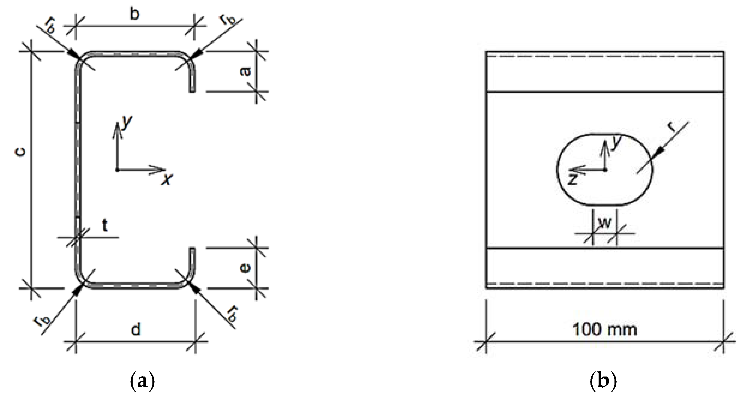
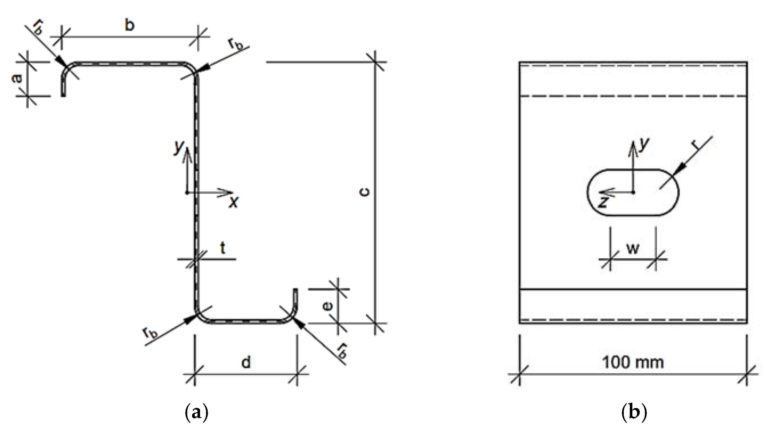
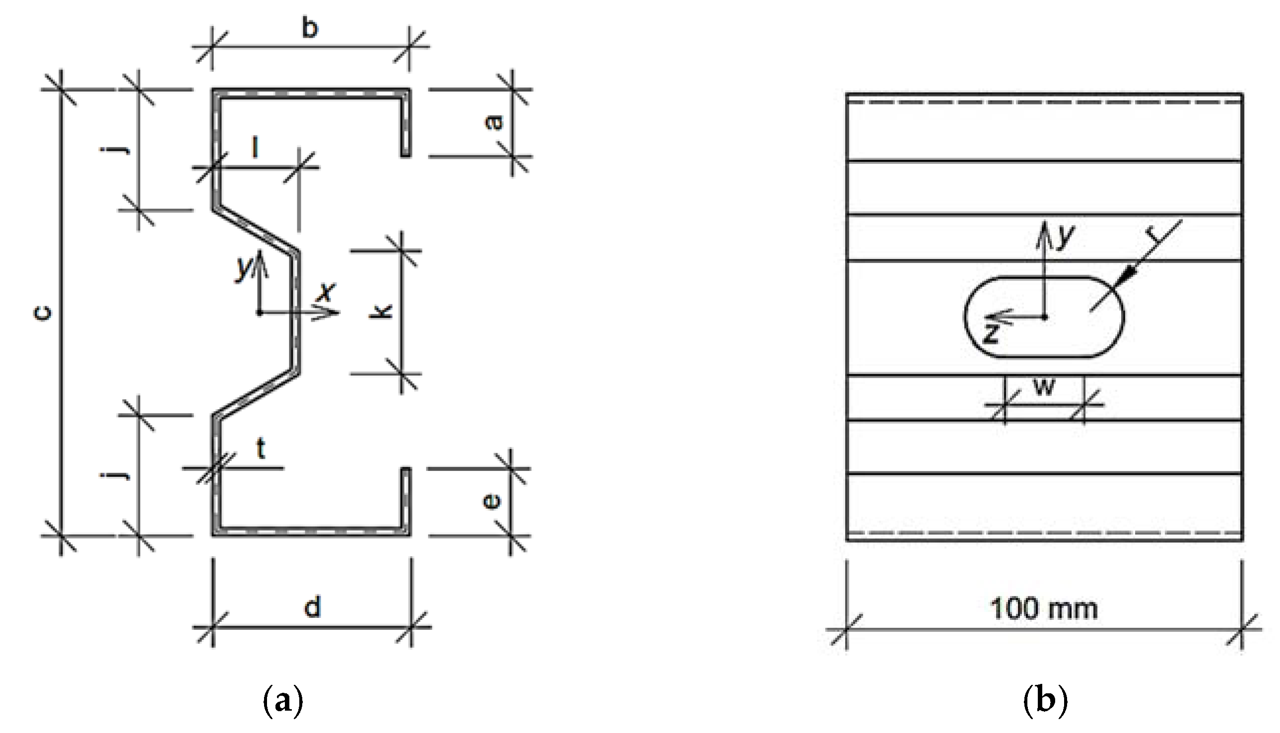
2.2. Parametric Models of Thin-Walled Cross-Sections
- b—upper flange width
- c—web height
- d—lower flange width
- t—thin-walled sheet
- w—length of the rectangular part of the hole
- r—radius of the hole
- b—upper/lower flange width
- c—overall height
- j—non-perforated height of the web
- k—perforation height
- l—web perforation depth
2.3. Numerical Homogenization Technique
2.4. Optimization Methods Used
2.4.1. Sequential Quadratic Programming
2.4.2. Radial Basis Function Network
2.5. Submodelling Sampling
2.5.1. Systematic Exploration
2.5.2. Optimal Latin Hypercube Sampling
2.6. Surrogate Model
3. Results
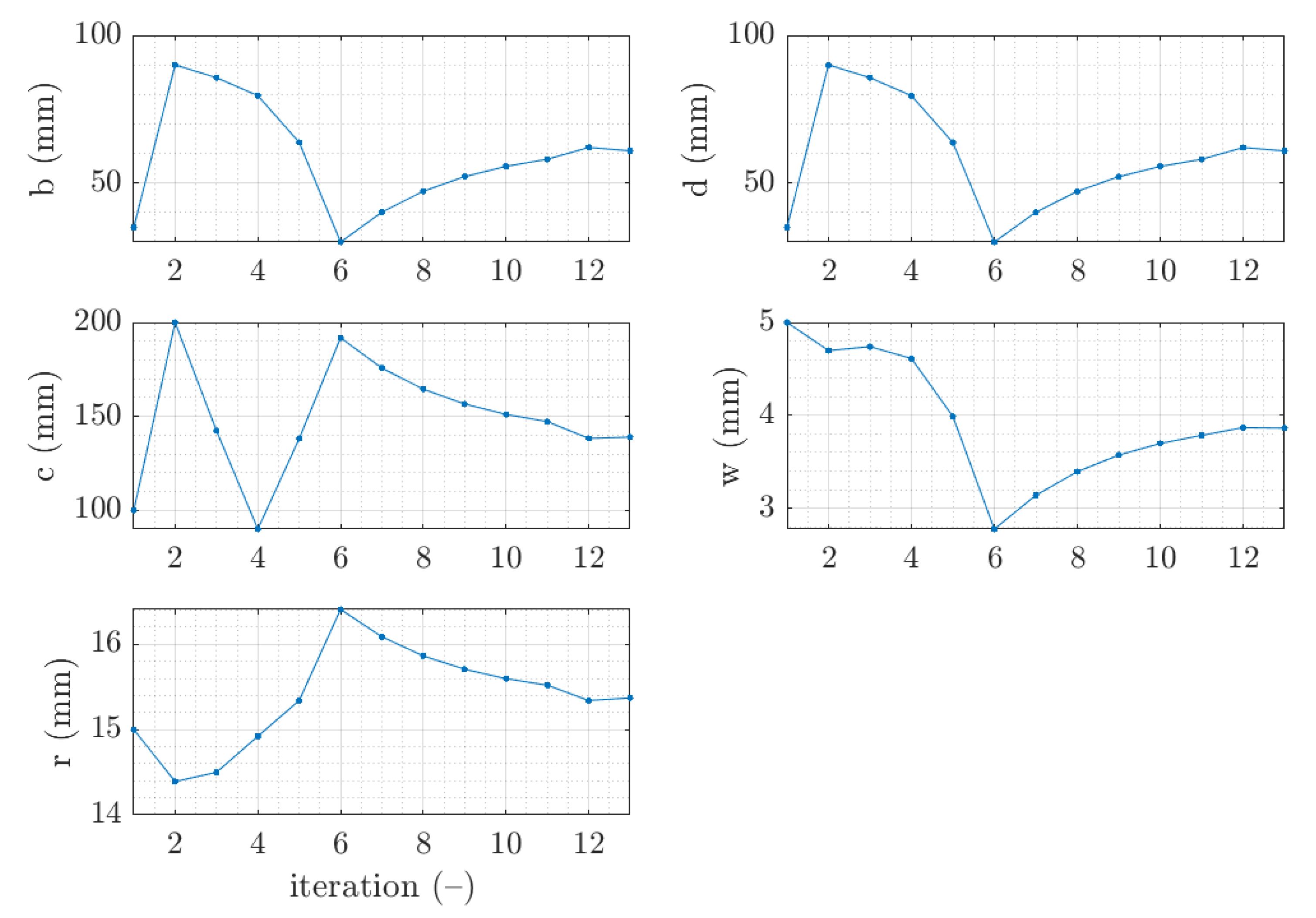
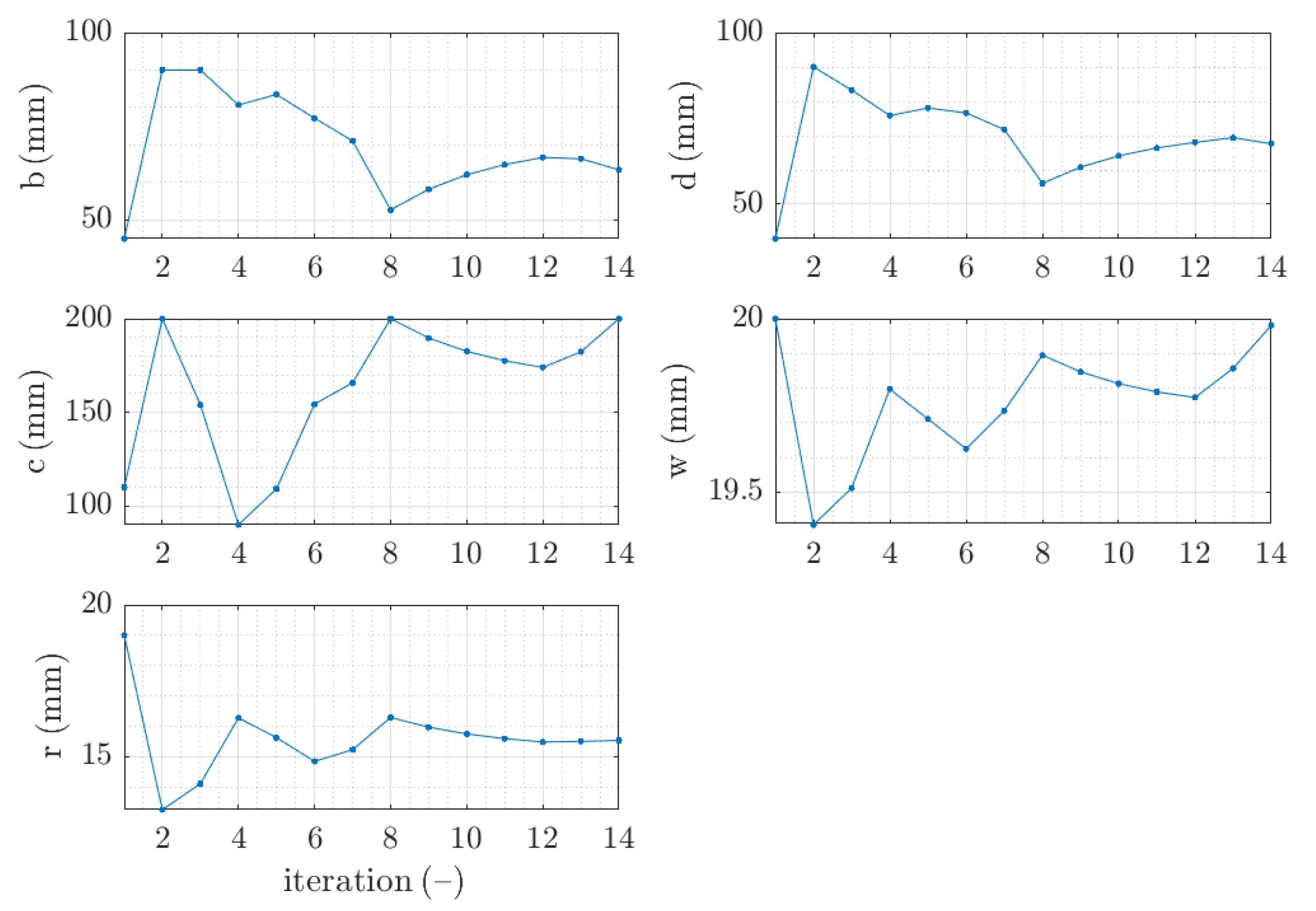
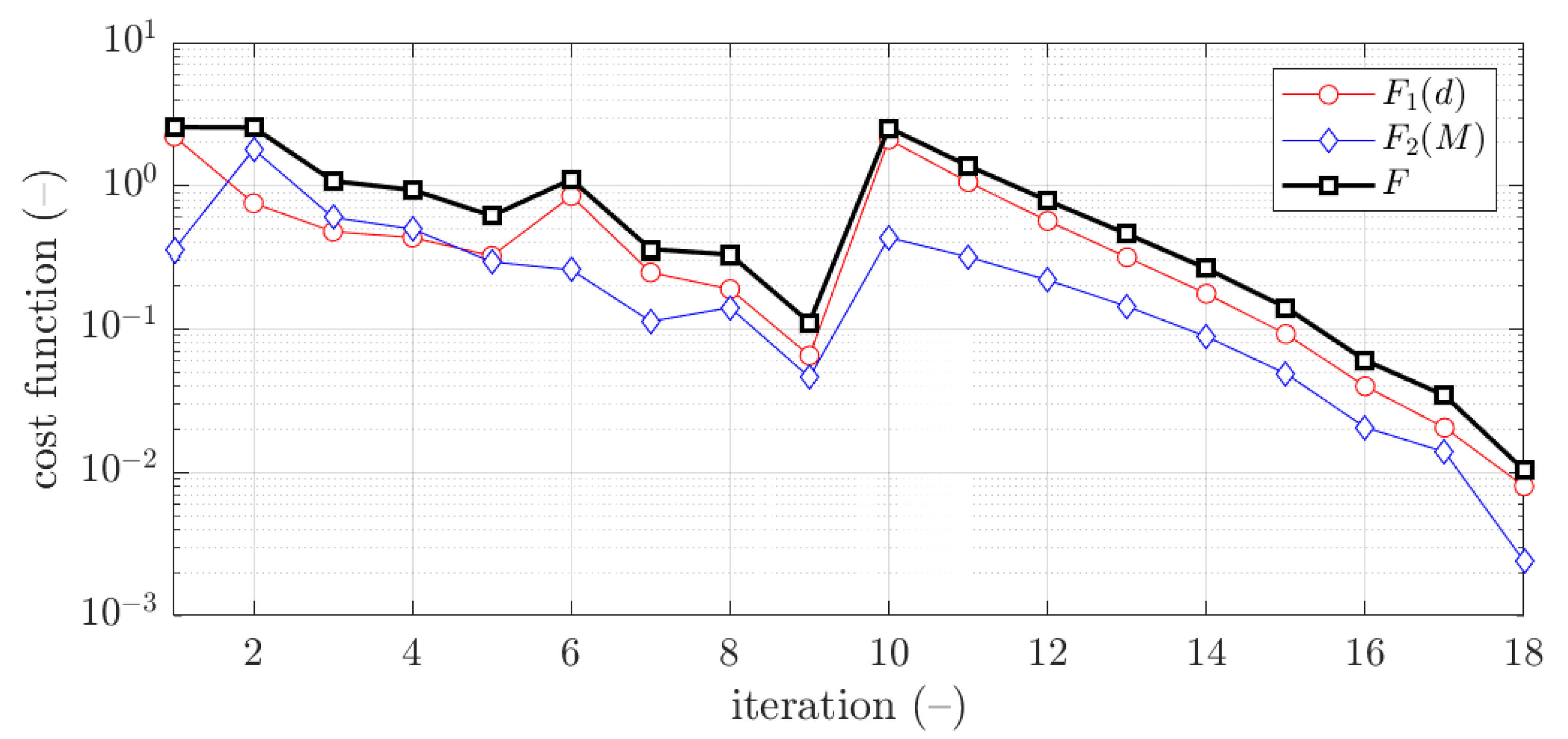
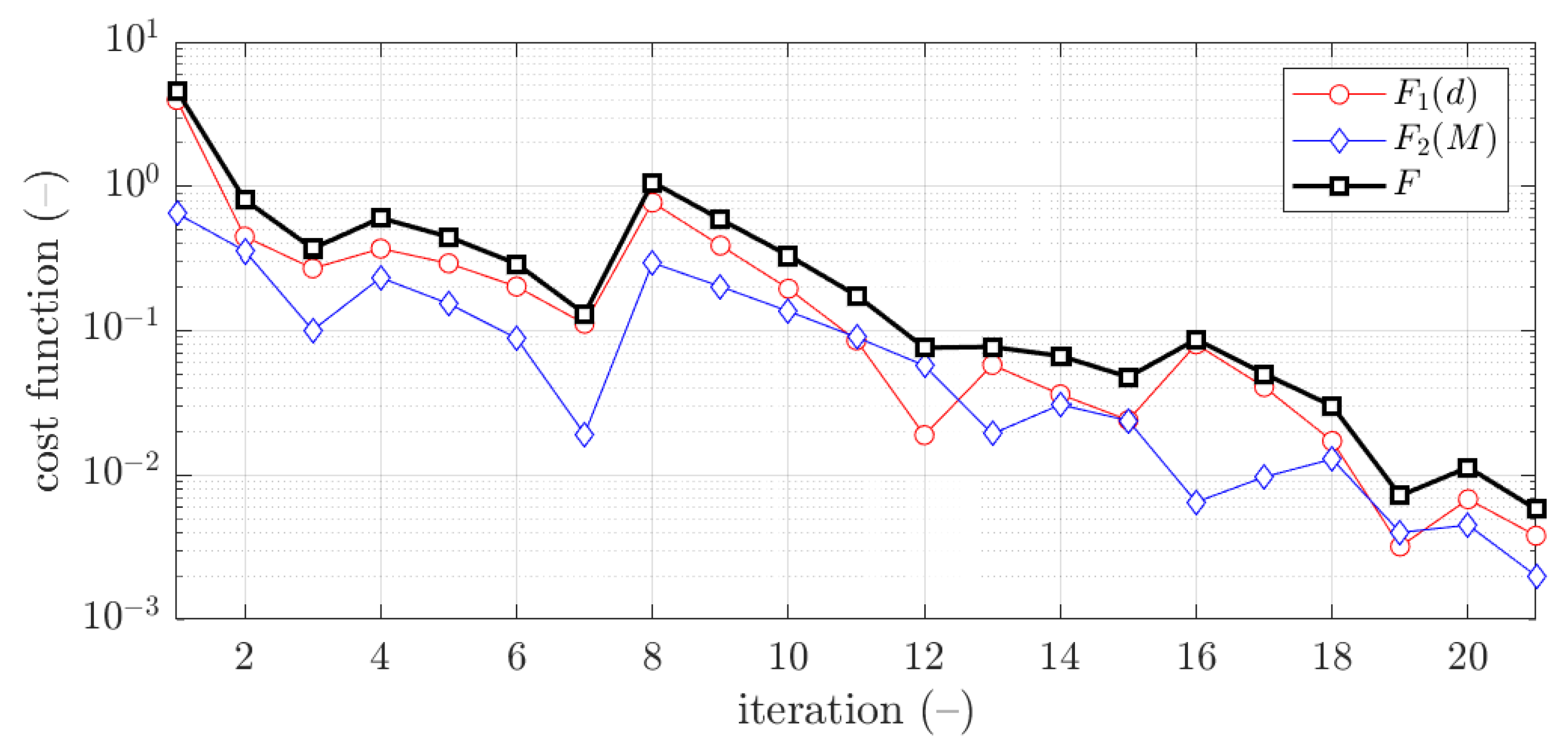
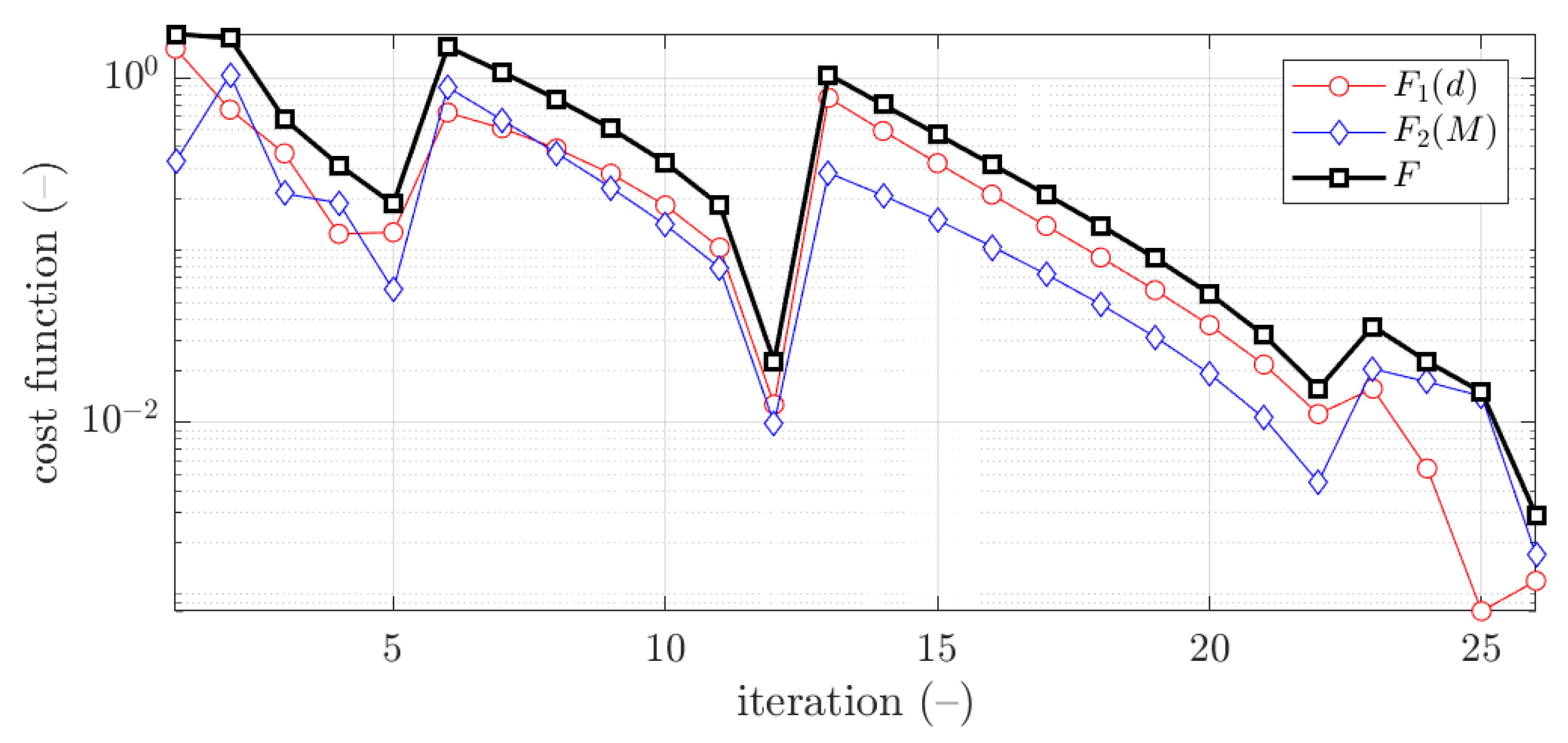
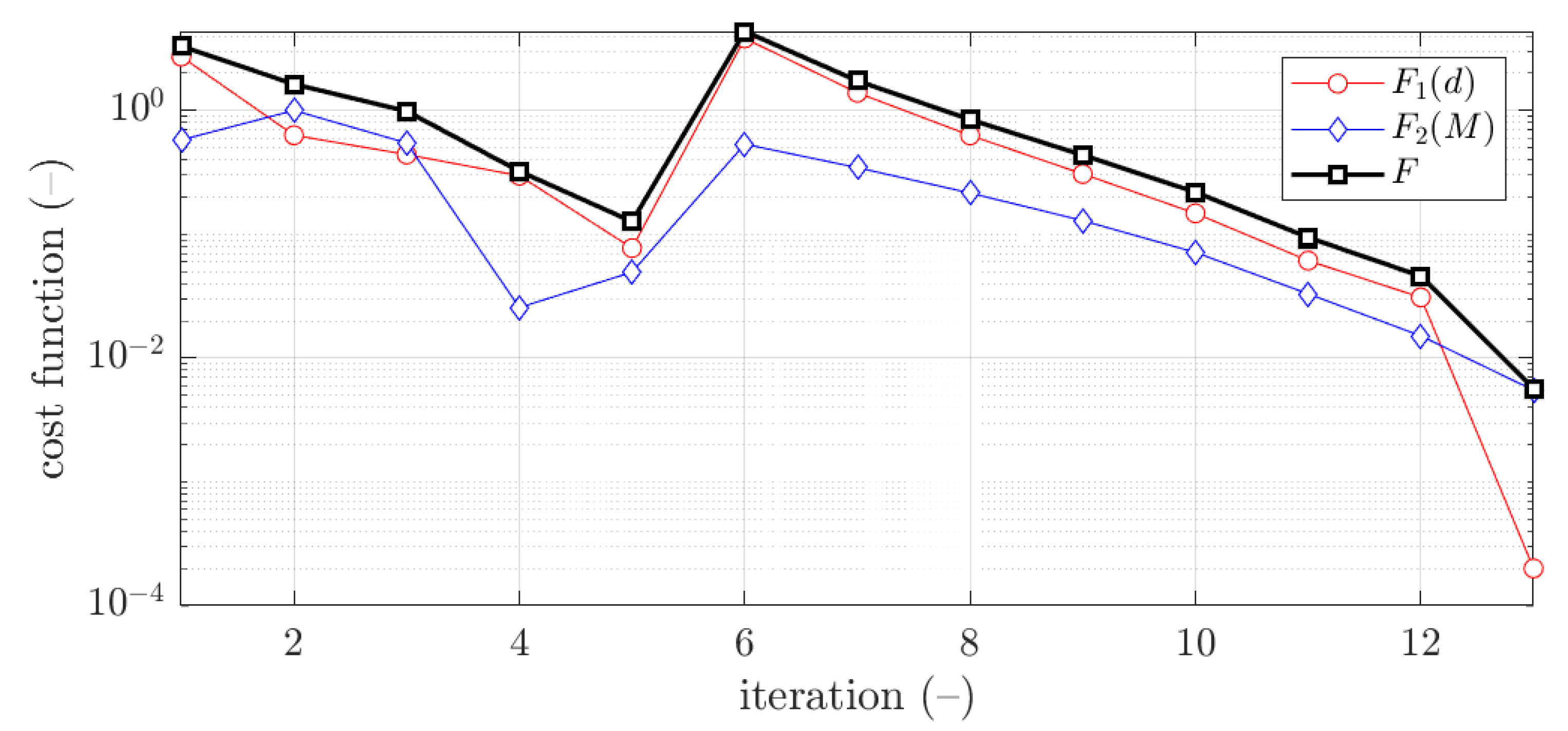
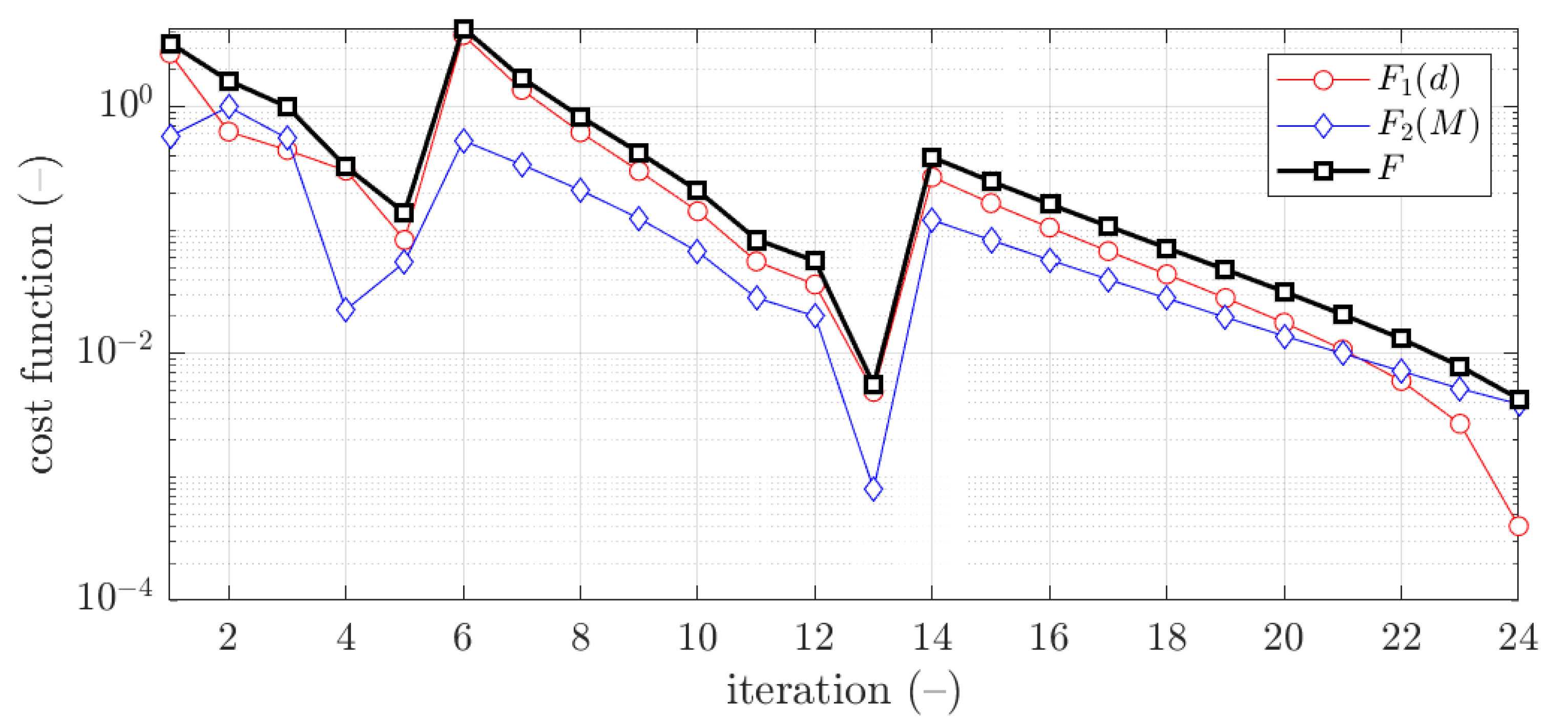
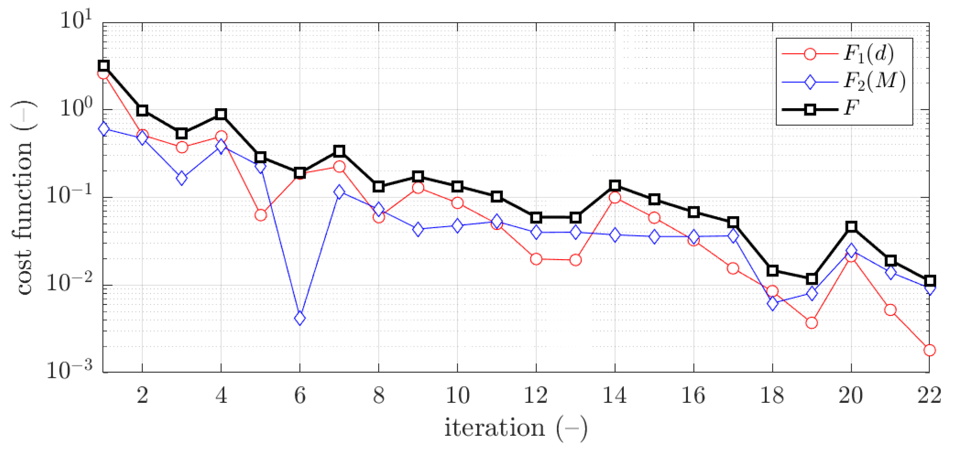
- design parameters are passed to the objective function (due to initial guess or optimization update, Equation (21))
- these design parameters are used to compute, via numerical homogenization, the effective stiffnesses (Equation (10))
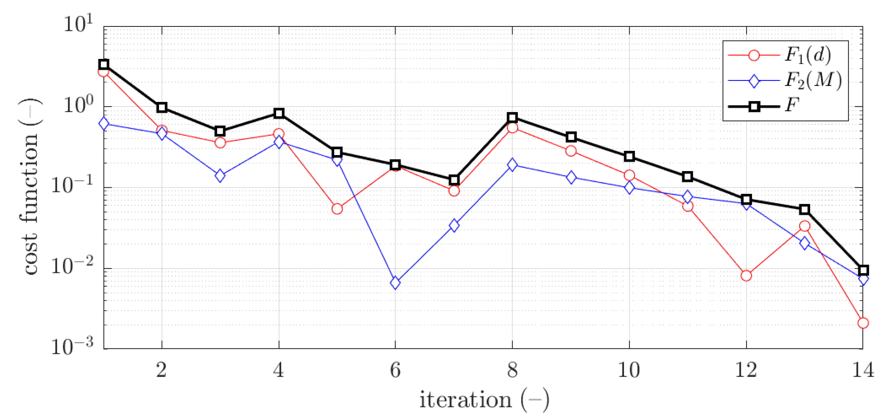
- these effective stiffnesses are used in Equations (2) and (3) to compute the objective function values , Equation (5), at each iteration step of the optimization process
- is minimized according to Equations from (13) to (21).
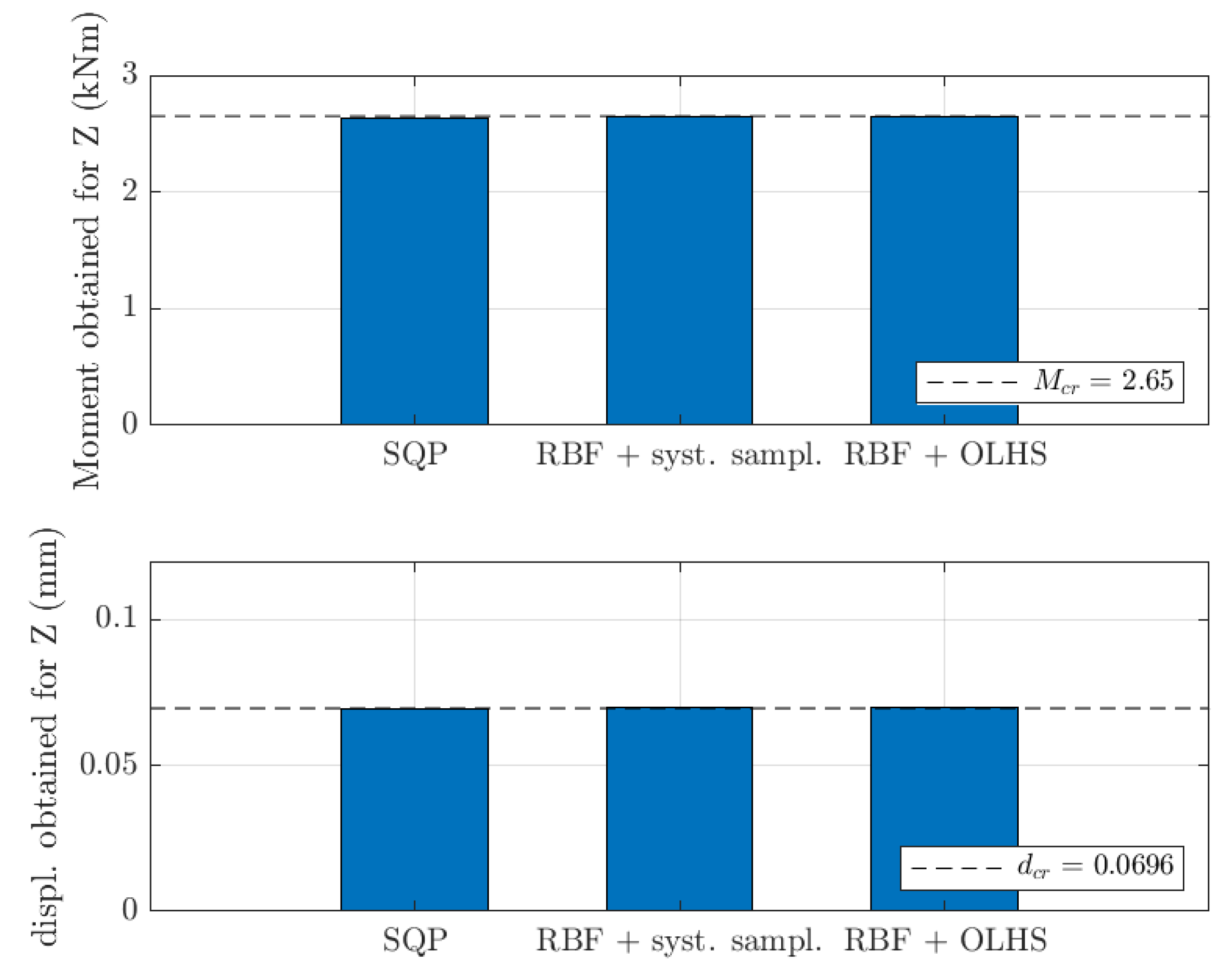
3.1. Traditional Optimization with SQP Minimization Algorithm
3.1.1. Z Profile
3.1.2. C Profile
3.1.3. Σ. Profile
3.2. Optimization with Radial Basis Function Metamodeling Feed with Systematic Sampling Data
3.2.1. Z Profile
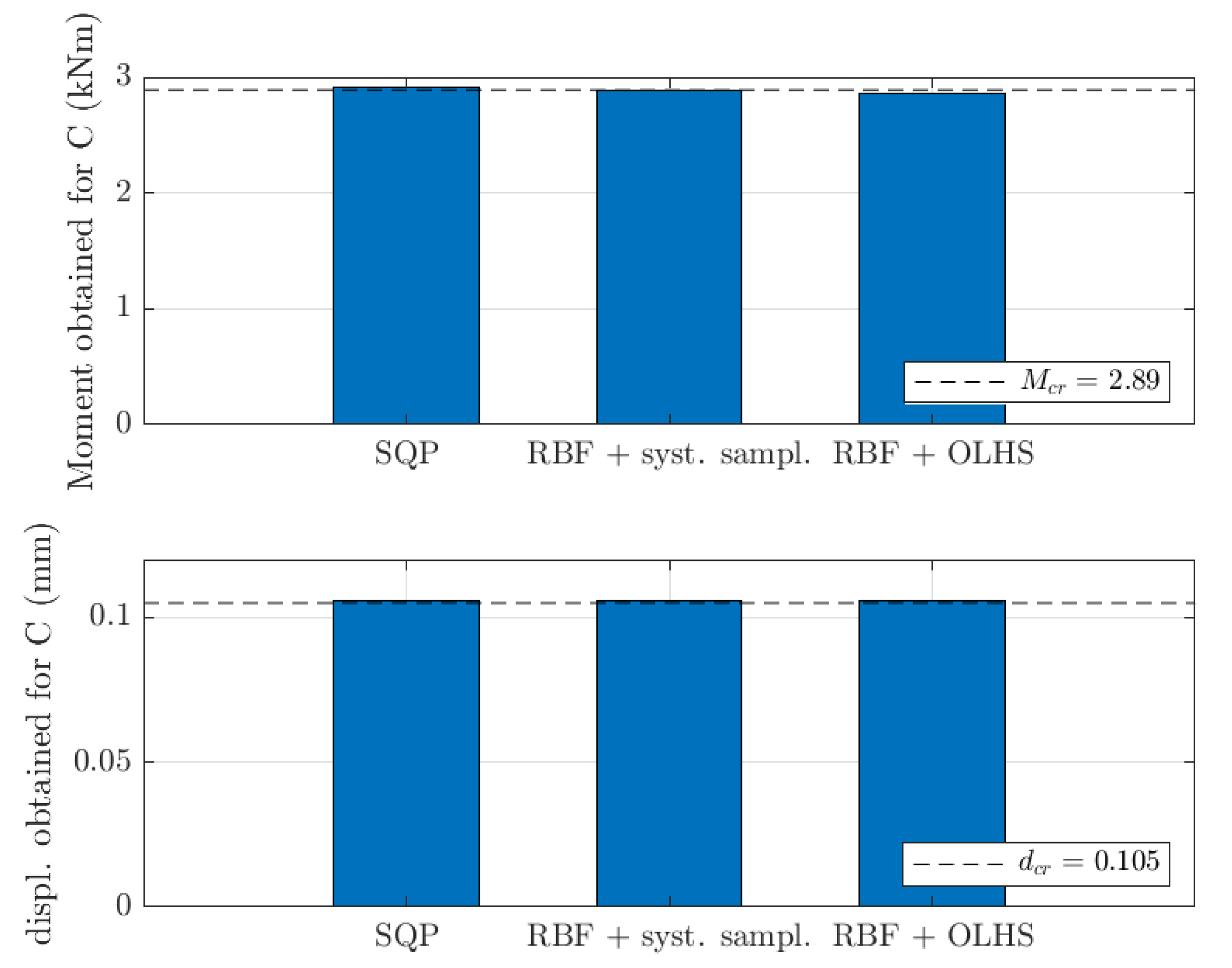
3.2.2. C Profile
3.3. Optimization with Radial Basis Function Metamodeling Feed with Optimal Latin Hypercube Sampling Data
3.3.1. Z Profile
3.3.2. C Profile
4. Discussion
5. Conclusions
Author Contributions
Funding
Institutional Review Board Statement
Informed Consent Statement
Data Availability Statement
Acknowledgments
Conflicts of Interest
References
- Ciesielczyk, K.; Studziński, R. Experimental and numerical investigation of stabilization of thin-walled Z-beams by sandwich panels. J. Constr. Steel Res. 2017, 133, 77–83. [Google Scholar] [CrossRef]
- Bihina, G.; Zhao, B.; Bouchaïr, A. Behaviour of composite steel–concrete cellular beams in fire. Eng. Struct. 2013, 56, 2217–2228. [Google Scholar] [CrossRef]
- Camotin, D.; Basaglia, C.; Silvestre, N. GBT buckling analysis of thin-walled steel frames: A state-of-the-art report. Thin-Walled Struct. 2010, 48, 726–743. [Google Scholar] [CrossRef]
- Yoon, K.; Lee, P.S.; Kim, D.N. An efficient warping model for elastoplastic torsional analysis of composite beams. Compos. Struct. 2017, 178, 37–49. [Google Scholar] [CrossRef]
- Genoese, A.; Genoese, A.; Bilotta, A.; Garcea, G. A generalized model for heterogeneous and anisotropic beams including section distortions. Thin-Walled Struct. 2014, 74, 85–103. [Google Scholar] [CrossRef]
- Addessi, D.; Di Re, P.; Cimarello, G. Enriched beam finite element models with torsion and shear warping for the analysis of thin-walled struc-tures. Thin-Walled Struct. 2021, 159, 107259. [Google Scholar] [CrossRef]
- Mrówczyński, D.; Gajewski, T.; Garbowski, T. The generalized constitutive law in nonlinear structural analysis of steel frames. In Modern Trends in Research on Steel, Aluminium and Composite Structures, Proceedings of the 14th International Conference on Metal Structures, Poznań, Poland, 16–18 June 2021; Giżejowski, M.A., Kozłowski, A., Chybiński, M., Rzeszut, K., Studziński, R., Szumigała, M., Eds.; Routledge Taylor and Francis Group: Leiden, The Netherlands, 2021; pp. 120–126. [Google Scholar] [CrossRef]
- Mrówczyński, D.; Gajewski, T.; Garbowski, T. Application of the generalized nonlinear constitutive law in 2D shear flexible beam structures. Arch. Civ. Eng. 2021, 67, 157–176. [Google Scholar] [CrossRef]
- Staszak, N.; Gajewski, T.; Garbowski, T. Generalized nonlinear constitutive law applied to steel trapezoidal sheet plates. In Modern Trends in Research on Steel, Aluminium and Composite Structures, Proceedings of the 14th International Conference on Metal Structures (ICMS2021), Poznan, Poland, 16–18 June 2021; Giżejowski, M.A., Kozłowski, A., Chybiński, M., Rzeszut, K., Studziński, R., Szumigała, M., Eds.; Routledge Taylor and Francis Group: Leiden, The Netherlands, 2021; pp. 185–191. [Google Scholar] [CrossRef]
- Staszak, N.; Garbowski, T.; Ksit, B. Application of the Generalized Nonlinear Constitutive Law to Hollow-Core. Preprints 2021, 2021070672. [Google Scholar] [CrossRef]
- Hohe, J. A direct homogenisation approach for determination of the stiffness matrix for microheterogeneous plates with application to sandwich panels. Compos. Part B Eng. 2003, 34, 615–626. [Google Scholar] [CrossRef]
- Buannic, N.; Cartraud, P.; Quesnel, T. Homogenization of corrugated core sandwich panels. Compos. Struct. 2003, 59, 299–312. [Google Scholar] [CrossRef] [Green Version]
- Cartraud, P.; Messager, T. Computational homogenization of periodic beam-like structures. Int. J. Solid Struct. 2006, 43, 686–696. [Google Scholar] [CrossRef] [Green Version]
- Biancolini, M.E. Evaluation of equivalent stiffness properties of corrugated board. Compos. Struct. 2005, 69, 322–328. [Google Scholar] [CrossRef]
- Garbowski, T.; Gajewski, T. Determination of transverse shear stiffness of sandwich panels with a corrugated core by numerical homogenization. Materials 2021, 14, 1976. [Google Scholar] [CrossRef] [PubMed]
- Staszak, N.; Garbowski, T.; Szymczak-Graczyk, A. Solid Truss to Shell Numerical Homogenization of Prefabricated Composite Slabs. Materials 2021, 14, 4120. [Google Scholar] [CrossRef] [PubMed]
- Garbowski, T.; Knitter-Piątkowska, A.; Mrówczyński, D. Numerical Homogenization of Multi-Layered Corrugated Cardboard with Creasing or Perforation. Materials 2021, 14, 3786. [Google Scholar] [CrossRef] [PubMed]
- Staszak, N.; Gajewski, T.; Garbowski, T. Shell-to-Beam Numerical Homogenization of 3D Thin-Walled Perforated Beams. Materials 2022, 15, 1827. [Google Scholar] [CrossRef]
- Gesualdo, A.; Iannuzzo, A.; Pucillo, G.P.; Penta, F. A direct technique for the homogenization of periodic beam-like structures by transfer matrix eigen-analysis. Lat. Am. J. Solids Struct. 2018, 15, 1–30. [Google Scholar] [CrossRef] [Green Version]
- Reda, H.; Alavi, S.E.; Nasimsobhan, M.; Ganghoffer, J.F. Homogenization towards chiral Cosserat continua and applications to enhanced Timoshenko beam theories. Mech. Mater. 2021, 155, 21. [Google Scholar] [CrossRef]
- Tsavdaridis, K.D.; D’Mello, C. Optimisation of novel elliptically-based web opening shapes of perforated steel beams. J. Constr. Steel Res. 2012, 76, 39–53. [Google Scholar] [CrossRef]
- Allaire, G.; Geoffroy-Donders, P.; Pantz, O. Topology optimization of modulated and oriented periodic microstructures by the homogenization method. Comput. Math. Appl. 2019, 78, 2197–2229. [Google Scholar] [CrossRef] [Green Version]
- Wang, Z.P.; Poh, L.H. Optimal form and size characterization of planar isotropic petal-shaped auxetics with tunable effective properties using IGA. Compos. Struct. 2018, 201, 486–502. [Google Scholar] [CrossRef]
- Tserpes, K.I.; Chanteli, A. Parametric numerical evaluation of the effective elastic properties of carbon nanotube-reinforced polymers. Compos. Struct. 2013, 99, 366–374. [Google Scholar] [CrossRef]
- Vinot, P.; Cogan, S.; Piranda, J. Shape optimization of thin-walled beam-like structures. Thin-Walled Struct. 2001, 39, 611–630. [Google Scholar] [CrossRef]
- Tsavdaridis, K.D.; Kingman, J.J.; Toropov, V.V. Application of structural topology optimisation to perforated steel beams. Comput. Struct. 2015, 158, 108–123. [Google Scholar] [CrossRef] [Green Version]
- Geoffroy-Donders, P.; Allaire, G.; Pantz, O. 3-d topology optimization of modulated and oriented periodic microstructures by the homogenization method. J. Comput. Phys. 2020, 401, 108994. [Google Scholar] [CrossRef] [Green Version]
- Magnucki, K.; Monczak, T. Optimum shape of the open cross-section of a thin-walled beam. Eng. Optim. 2000, 32, 335–351. [Google Scholar] [CrossRef]
- Parastesh, H.; Hajirasouliha, I.; Taji, H.; Sabbagh, A.B. Shape optimization of cold-formed steel beam-columns with practical and manufacturing constraints. J. Constr. Steel Res. 2019, 155, 249–259. [Google Scholar] [CrossRef]
- Fiore, A.; Marano, G.C.; Greco, R.; Mastromarino, E. Structural optimization of hollow-section steel trusses by differential evolution algorithm. Int. J. Steel Struct. 2016, 16, 411–423. [Google Scholar] [CrossRef]
- Lian, Y.; Uzzaman, A.; Lim, J.B.; Abdelal, G.; Nash, D.; Young, B. Effect of web holes on web crippling strength of cold-formed steel channel sections under end-one-flange loading condition–Part I: Tests and finite element analysis. Thin-Walled Struct. 2016, 107, 443–452. [Google Scholar] [CrossRef] [Green Version]
- Chuda-Kowalska, M.; Gajewski, T.; Garbowski, T. The mechanical characterization of orthotropic elastic parameters of a foam by the mixed experimental-numerical analysis. J. Theor. Appl. Mech. 2015, 53, 383–394. [Google Scholar] [CrossRef] [Green Version]
- Sielicki, P.W.; Sumelka, W.; Łodygowski, T. Close Range Explosive Loading on Steel Column in the Framework of Anisotropic Viscoplasticity. Metals 2019, 9, 454. [Google Scholar] [CrossRef] [Green Version]
- Kołodziej, J.A.; Grabski, J.K. Many names of the Trefftz method. Eng. Anal. Bound. Elem. 2018, 96, 169–178. [Google Scholar] [CrossRef]
- Grabski, J.K.; Mrozek, A. Identification of elastoplastic properties of rods from torsion test using meshless methods and a metaheuristic. Comput. Math. Appl. 2021, 92, 149–158. [Google Scholar] [CrossRef]
- Schittkowski, K. NLQPL: A FORTRAN subroutine solving constrained nonlinear programming problems. Ann. Oper. Res. 1986, 5, 485–500. [Google Scholar] [CrossRef]
- Biggs, M.C. Constrained minimization using recursive quadratic programming. In Towards Global Optimization; North-Holland: Amsterdam, The Netherlands, 1975. [Google Scholar]
- Han, S.P. A globally convergent method for nonlinear programming. J. Optim. Theory Appl. 1977, 22, 297–309. [Google Scholar] [CrossRef] [Green Version]
- Powell, M.J.D. The convergence of variable metric methods for nonlinearly constrained optimization calculations. In Proceedings of the Special Interest Group on Mathematical Programming Symposium Conducted by the Computer Sciences Department at the University of Wisconsin–Madison, Madison, WI, USA, 11–13 July 1977; Academic Press: Cambridge, MA, USA, 1978. [Google Scholar] [CrossRef]
- Powell, M.J.D. A fast algorithm for nonlinearly constrained optimization calculations. Numer. Anal. 1978, 630, 144–157. [Google Scholar]
- Nocedal, J.; Wright, S.J. Numerical Optimization, 2nd ed.; Springer Series in Operations Research; Springer: Berlin/Heidelberg, Germany, 2006. [Google Scholar]
- Deep Learning Toolbox. Available online: https://www.mathworks.com/help/deeplearning/ug/radial-basis-neural-networks (accessed on 24 February 2022).
- Jin, R.; Chen, W.; Sudjianto, A. An efficient algorithm for constructing optimal design of computer experiments. J. Stat. Plan. Inference 2005, 134, 268–287. [Google Scholar] [CrossRef]


| Boundary | Profile | b (mm) | d (mm) | c (mm) | w (mm) | r (mm) |
|---|---|---|---|---|---|---|
| Z, C | 30 | 30 | 90 | 0 | 5 | |
| 90 | 90 | 200 | 24 | 20 | ||
| Boundary | Profile | b and d (mm) | c (mm) | j (mm) | k (mm) | l (mm) |
| Σ | 30 | 90 | 20 | 20 | 5 | |
| 90 | 200 | 45 | 80 | 45 |
| No. | Profile | b (mm) | d (mm) | c (mm) | w (mm) | r (mm) |
|---|---|---|---|---|---|---|
| Z, C | 45 | 40 | 110 | 20 | 19 | |
| Z, C | 35 | 35 | 140 | 5 | 5 | |
| Z, C | 30 | 65 | 90 | 5 | 15 | |
| Z, C | 35 | 35 | 100 | 5 | 15 | |
| Z, C | 45 | 30 | 150 | 10 | 5 | |
| No. | Profile | b and d (mm) | c (mm) | j (mm) | k (mm) | l (mm) |
| Σ | 80 | 150 | 37.5 | 50 | 50 | |
| Σ | 30 | 120 | 20 | 40 | 20 | |
| Σ | 60 | 110 | 37.5 | 20 | 35 | |
| Σ | 45 | 170 | 20 | 20 | 10 | |
| Σ | 55 | 135 | 30 | 30 | 30 |
| No. | t (mm) | b (mm) | d (mm) | c (mm) | w (mm) | r (mm) | |
|---|---|---|---|---|---|---|---|
| 1 | 1.5 | 82.97 | 84.08 | 124.01 | 19.64 | 19.16 | 0.0085 |
| 2 | 87.92 | 87.92 | 113.67 | 4.82 | 5.06 | 0.0084 | |
| 3 | 63.56 | 69.52 | 200 | 4.53 | 12.69 | 0.0554 | |
| 4 | 85.14 | 85.14 | 119.31 | 5.6 | 16.38 | 0.0079 | |
| 5 | 90.0 | 89.6 | 112.42 | 9.19 | 5.26 | 0.0259 | |
| 1 | 2.0 | 60.8 | 57.02 | 155.88 | 19.92 | 18.23 | 0.0218 |
| 2 | 90.0 | 90.0 | 200.0 | 4.98 | 5.02 | 1.6343 | |
| 3 | 55.78 | 62.78 | 149.35 | 4.62 | 13.55 | 0.0068 | |
| 4 | 60.9 | 60.87 | 138.94 | 3.86 | 15.37 | 0.0057 | |
| 5 | 78.85 | 48.76 | 122.68 | 9.84 | 6.2 | 0.0058 |
| No. | t (mm) | b (mm) | d (mm) | c (mm) | w (mm) | r (mm) | |
|---|---|---|---|---|---|---|---|
| 1 | 1.5 | 63.37 | 67.64 | 200 | 19.98 | 15.54 | 0.0095 |
| 2 | 89.45 | 89.15 | 96.69 | 5.22 | 5.32 | 0.1845 | |
| 3 | 43.47 | 88.0 | 130.68 | 4.85 | 14.33 | 0.0410 | |
| 4 | 64.77 | 65.81 | 200 | 5.67 | 14.85 | 0.0107 | |
| 5 | 85.14 | 50.86 | 129.97 | 9.16 | 5.26 | 0.1632 | |
| 1 | 2.0 | 61.26 | 60.1 | 145.55 | 20.17 | 16.73 | 0.0073 |
| 2 | 84.92 | 85.13 | 90 | 4.19 | 6.04 | 0.1345 | |
| 3 | 90 | 54.49 | 95.13 | 4.8 | 14.14 | 0.1093 | |
| 4 | 86.09 | 85.94 | 90 | 1.64 | 8.73 | 0.1341 | |
| 5 | 58.09 | 59.77 | 144.87 | 11.07 | 5.24 | 0.0112 |
| No. | t (mm) | b and d (mm) | c (mm) | j (mm) | k (mm) | l (mm) | |
|---|---|---|---|---|---|---|---|
| 1 | 1.5 | 64.51 | 90 | 34.23 | 45.87 | 45.0 | 0.1004 |
| 2 | 66.94 | 90 | 40.06 | 20.06 | 45.0 | 0.1104 | |
| 3 | 54.72 | 159.5 | 41.62 | 22.65 | 40.5 | 0.0733 | |
| 4 | 56.40 | 145.1 | 26.02 | 20.0 | 5.0 | 0.0260 | |
| 5 | 54.79 | 157.6 | 36.0 | 31.42 | 41.87 | 0.0719 | |
| 1 | 2.0 | 51.82 | 90.0 | 30.0 | 45.6 | 38.26 | 0.0280 |
| 2 | 50.49 | 90.0 | 43.35 | 20.0 | 41.39 | 0.0104 | |
| 3 | 53.48 | 90.0 | 35.70 | 20.0 | 34.98 | 0.0237 | |
| 4 | 51.77 | 107.5 | 31.26 | 20.77 | 20.95 | 0.0491 | |
| 5 | 53.43 | 90.0 | 35.71 | 32.40 | 30.48 | 0.0241 |
| No. | t (mm) | b (mm) | d (mm) | c (mm) | w (mm) | r (mm) | |
|---|---|---|---|---|---|---|---|
| 1 | 1.5 | 83.36 | 76.4 | 137.39 | 20.07 | 18.55 | 0.0902 |
| 2 | 87.56 | 87.55 | 114.15 | 4.74 | 7.09 | 0.0078 | |
| 3 | 58.31 | 74.06 | 200 | 4.55 | 13.19 | 0.0531 | |
| 4 | 86.46 | 86.45 | 117.42 | 4.96 | 15.89 | 0.0058 (0.0248) | |
| 5 | 90 | 83.52 | 115.2 | 9.91 | 6.44 | 0.0105 | |
| 1 | 2.0 | 61.6 | 59.43 | 142.02 | 19.68 | 17.15 | 0.009 |
| 2 | 66.6 | 66.55 | 117.29 | 5.14 | 6.98 | 0.0073 | |
| 3 | 60.69 | 57.7 | 152.2 | 4.62 | 13.33 | 0.0092 | |
| 4 | 60.7 | 60.7 | 140.52 | 5.04 | 15.82 | 0.0043 (0.0315) | |
| 5 | 64.71 | 58.91 | 132.61 | 10.15 | 6.5 | 0.0129 |
| No. | t (mm) | b (mm) | d (mm) | c (mm) | w (mm) | r (mm) | |
|---|---|---|---|---|---|---|---|
| 1 | 1.5 | 67.14 | 63.35 | 200 | 19.89 | 12.23 | 0.0111 |
| 2 | 90 | 90 | 98.89 | 3.95 | 14.14 | 0.1822 | |
| 3 | 40.7 | 80.65 | 167 | 4.52 | 13.9 | 0.0697 | |
| 4 | 69.52 | 68.63 | 158.7 | 3.61 | 18.29 | 0.1079 | |
| 5 | 83.8 | 33.78 | 157.93 | 10.48 | 14.52 | 0.0091(0.0144) | |
| 1 | 2.0 | 51.68 | 67.4 | 144.37 | 19.93 | 15.51 | 0.0024 (0.0030) |
| 2 | 81.11 | 79.27 | 90 | 6 | 14.41 | 0.1109 | |
| 3 | 90 | 54.99 | 95.02 | 4.81 | 14.31 | 0.1126 | |
| 4 | 90 | 78.81 | 90 | 10.53 | 20 | 0.0904 | |
| 5 | 64.53 | 53.92 | 145.78 | 10.12 | 10.83 | 0.0056 |
| No. | t (mm) | b (mm) | d (mm) | c (mm) | w (mm) | r (mm) | |
|---|---|---|---|---|---|---|---|
| 1 | 1.5 | 66.26 | 67.87 | 188.8 | 21.01 | 17.16 | 0.0772 |
| 2 | 87.48 | 87.29 | 114.64 | 4.95 | 5.79 | 0.0058 (0.0004) | |
| 3 | 56.16 | 75.61 | 200 | 4.4 | 12.17 | 0.0567 | |
| 4 | 82.95 | 80.55 | 122.36 | 5.61 | 15.07 | 0.0484 | |
| 5 | 90.0 | 85.63 | 113.75 | 10.7 | 5.0 | 0.0113 | |
| 1 | 2.0 | 62.29 | 56.38 | 151.84 | 19.98 | 17.8 | 0.0154 |
| 2 | 66.76 | 67.17 | 116.47 | 4.84 | 5.02 | 0.0084 | |
| 3 | 54.86 | 62.04 | 160.03 | 4.39 | 12.22 | 0.0221 | |
| 4 | 60.67 | 61.12 | 138.63 | 4.94 | 14.85 | 0.0098 | |
| 5 | 82.96 | 32.9 | 138.04 | 9.98 | 8.56 | 0.0072 (0.0069) |
| No. | t (mm) | b (mm) | d (mm) | c (mm) | w (mm) | r (mm) | |
|---|---|---|---|---|---|---|---|
| 1 | 1.5 | 66.85 | 64.74 | 192.81 | 20.61 | 14.46 | 0.0196 (0.0186) |
| 2 | 89.8 | 87.98 | 97.81 | 4.78 | 5.57 | 0.1855 | |
| 3 | 40.78 | 80.43 | 169.31 | 4.52 | 11.2 | 0.0546 | |
| 4 | 75.01 | 51.8 | 184.13 | 3.76 | 7.68 | 0.0224 | |
| 5 | 88.62 | 68.07 | 109.38 | 10.24 | 5.42 | 0.1993 | |
| 1 | 2.0 | 49.86 | 69.02 | 142.49 | 20.26 | 17.13 | 0.0163 |
| 2 | 63.0 | 90.0 | 90.0 | 5.92 | 7.39 | 0.1053 | |
| 3 | 90.0. | 53.76 | 95.26 | 4.7 | 13.38 | 0.1098 | |
| 4 | 90.0 | 90.0 | 90.0 | 24.0 | 20.0 | 0.0603 | |
| 5 | 59.61 | 59.32 | 144.03 | 9.77 | 7.54 | 0.0029 (0.0011) |
Publisher’s Note: MDPI stays neutral with regard to jurisdictional claims in published maps and institutional affiliations. |
© 2022 by the authors. Licensee MDPI, Basel, Switzerland. This article is an open access article distributed under the terms and conditions of the Creative Commons Attribution (CC BY) license (https://creativecommons.org/licenses/by/4.0/).
Share and Cite
Gajewski, T.; Staszak, N.; Garbowski, T. Parametric Optimization of Thin-Walled 3D Beams with Perforation Based on Homogenization and Soft Computing. Materials 2022, 15, 2520. https://doi.org/10.3390/ma15072520
Gajewski T, Staszak N, Garbowski T. Parametric Optimization of Thin-Walled 3D Beams with Perforation Based on Homogenization and Soft Computing. Materials. 2022; 15(7):2520. https://doi.org/10.3390/ma15072520
Chicago/Turabian StyleGajewski, Tomasz, Natalia Staszak, and Tomasz Garbowski. 2022. "Parametric Optimization of Thin-Walled 3D Beams with Perforation Based on Homogenization and Soft Computing" Materials 15, no. 7: 2520. https://doi.org/10.3390/ma15072520
APA StyleGajewski, T., Staszak, N., & Garbowski, T. (2022). Parametric Optimization of Thin-Walled 3D Beams with Perforation Based on Homogenization and Soft Computing. Materials, 15(7), 2520. https://doi.org/10.3390/ma15072520