
A Novel Method for the Determination of the Lateral Dimensions of 2D Rectangular Flakes


Abstract
:1. Introduction
- (i)
- Flakes are of rectangular shape and of uniform size;
- (ii)
- Flakes are parallel to each other;
- (iii)
- Flakes have random in-plane orientations in the interval .
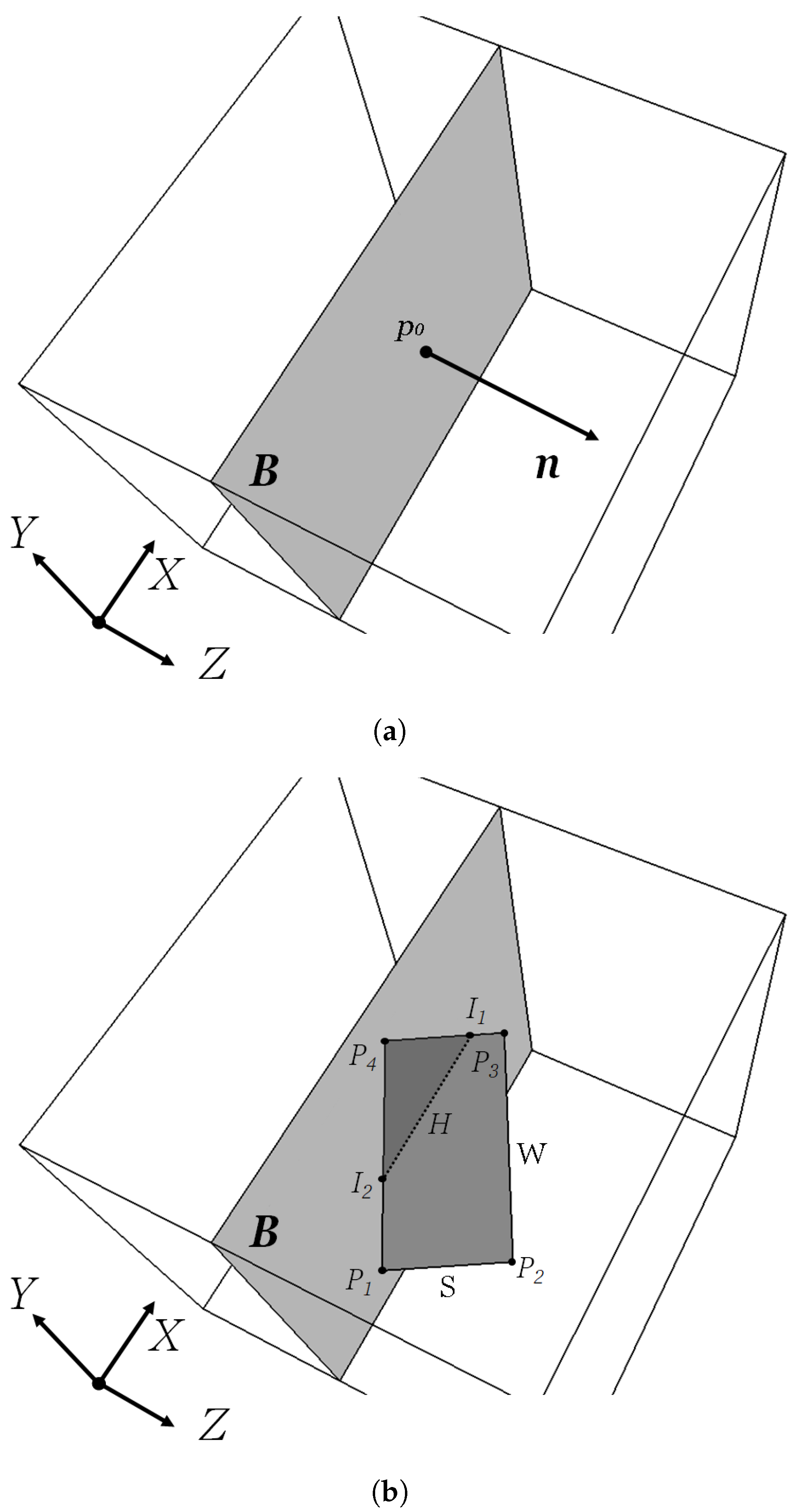
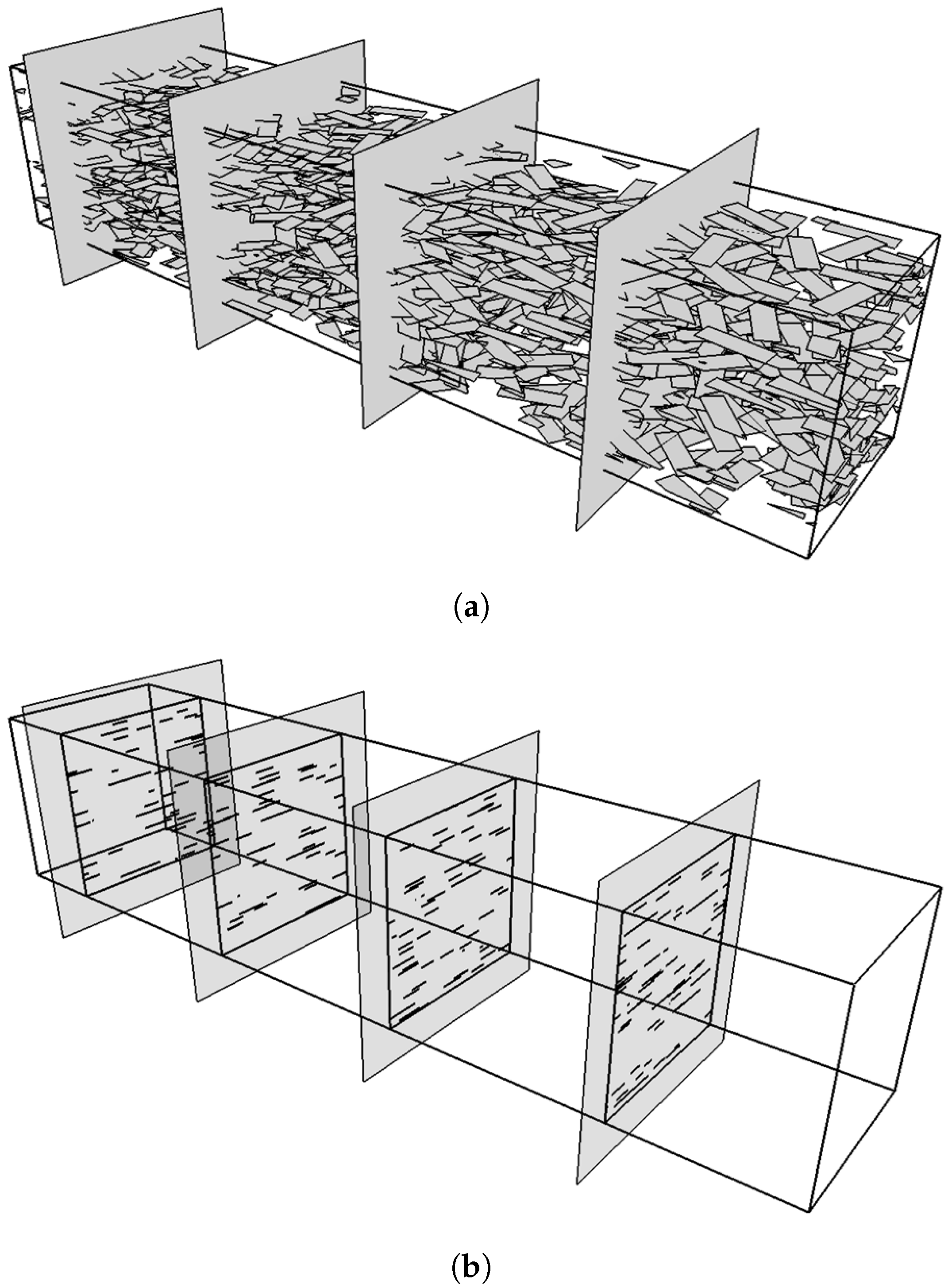
2. Geometry Generation and Numerical Sectioning
3. Theoretical Model for the Sectioning Process
- (i)
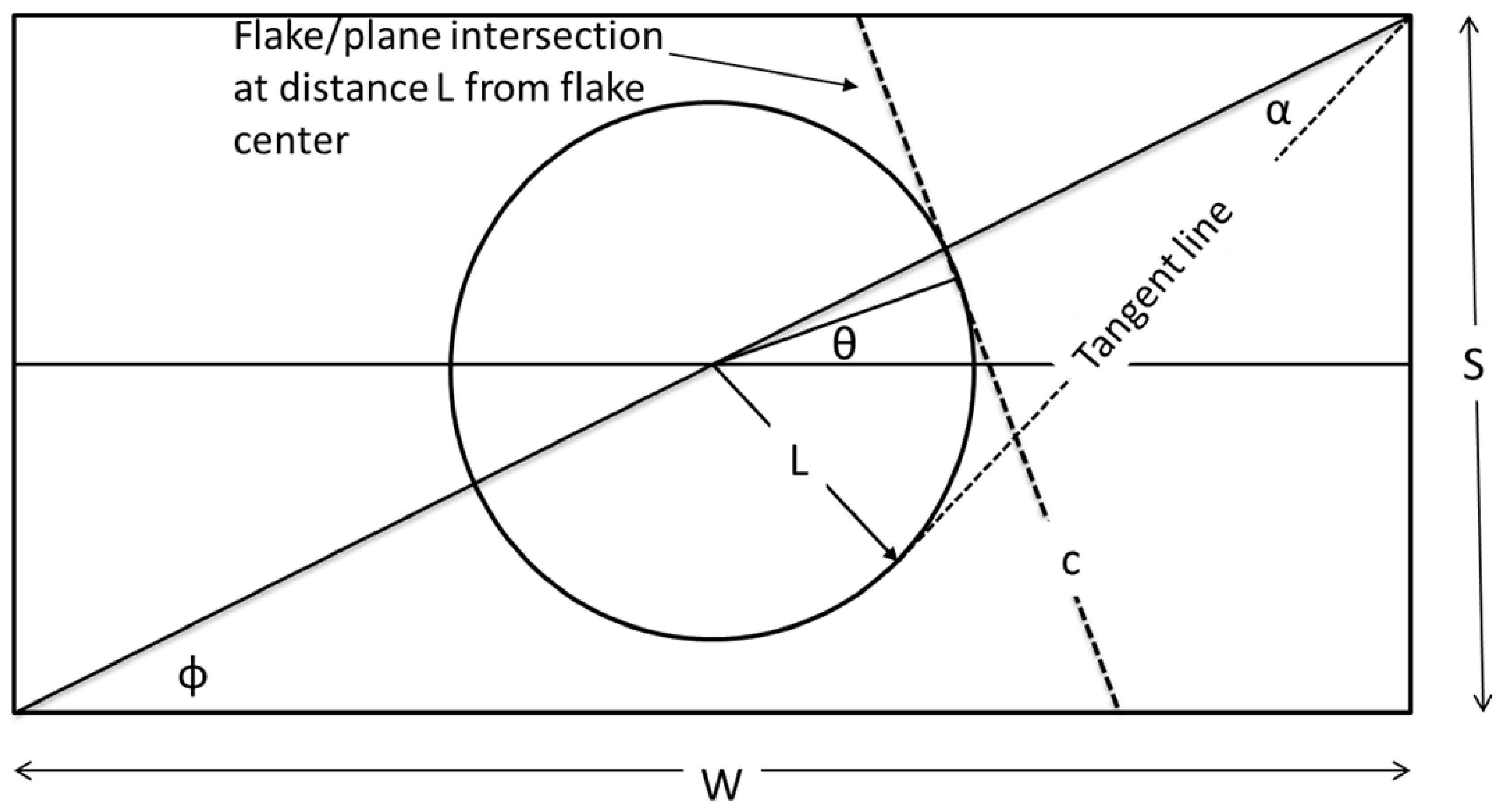
- (Figure 5a).In this case it is obvious that all lines tangent to the circle with radius (L) will intersect the rectangle; therefore, for there will be an intersecting line for all , . We define as angles to the angles formed (counter-clockwise) between the long axis of the rectangle and the arc points 1–4, at which a tangent will pass through a corner of the rectangle, as shown in Figure 5a. It can be shown that , , , . It then follows that the intersection length can be calculated as:
- (a)
- (b)
- (c)
- (d)
- (e)
Equations (4), (6) and (8) represent the case when the cutting plane intersects two opposite sides of the rectangle, while Equations (5) and (7) represent the case when it intersects adjacent sides. Only Equations (5)–(7) are expected to produce long intersections, while Equations (4) and (8) might generate intersections with lengths comparable to S. - (ii)
- (Figure 5b).In this case, not all tangent lines to the circle of radius (L) will intersect the rectangle. From Figure 5b it is clear that no intersection will occur if . For all other values of the cutting plane will intersect the rectangle. It can be shown that , , , . In this case the intersection lengths are calculated as:
- (iii)
- (Figure 5c).The situation is similar to (ii) and the arcs at which no intersecting lines can be drawn are , , and . , , , . The intersection lengths are
4. Results and Discussion
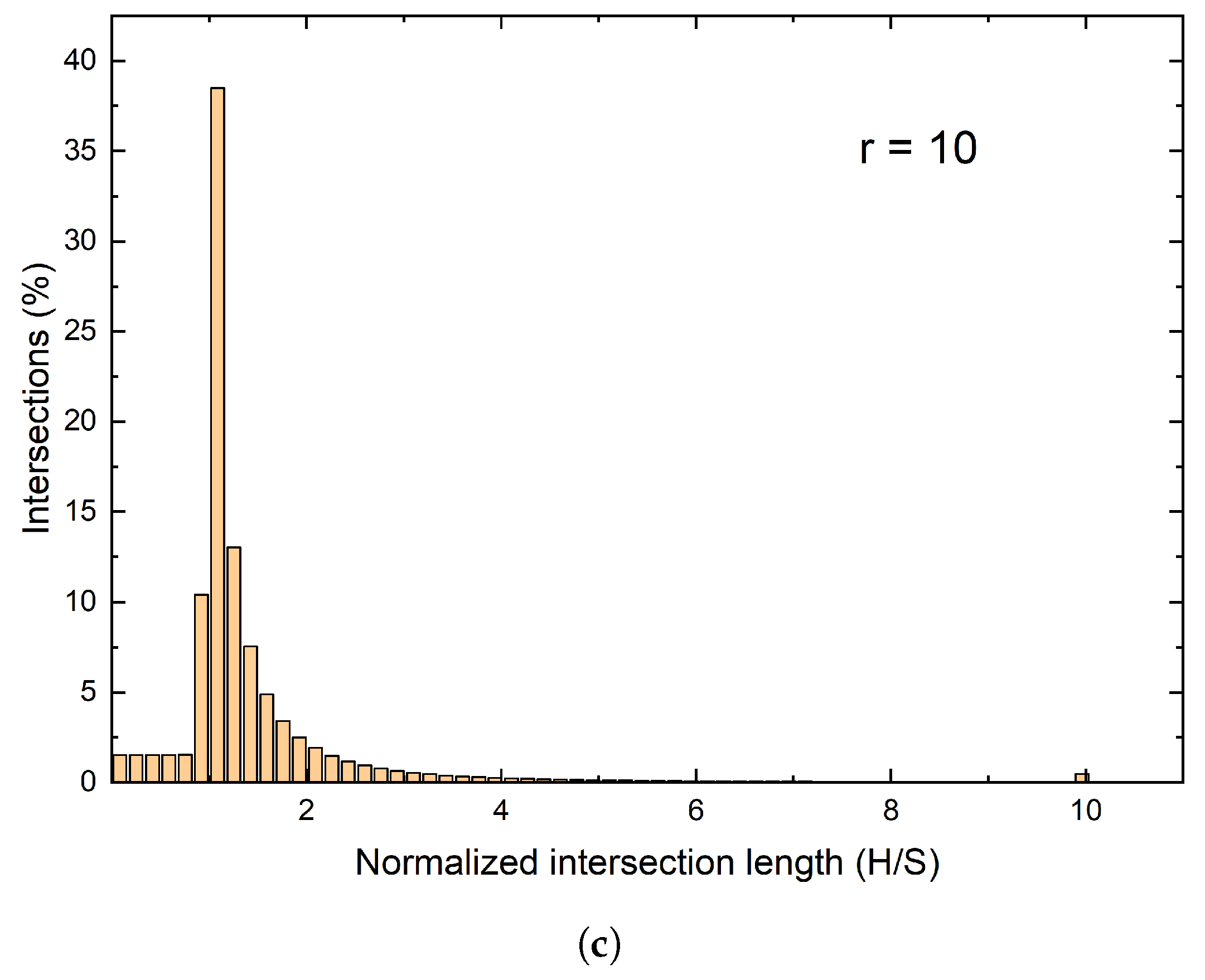
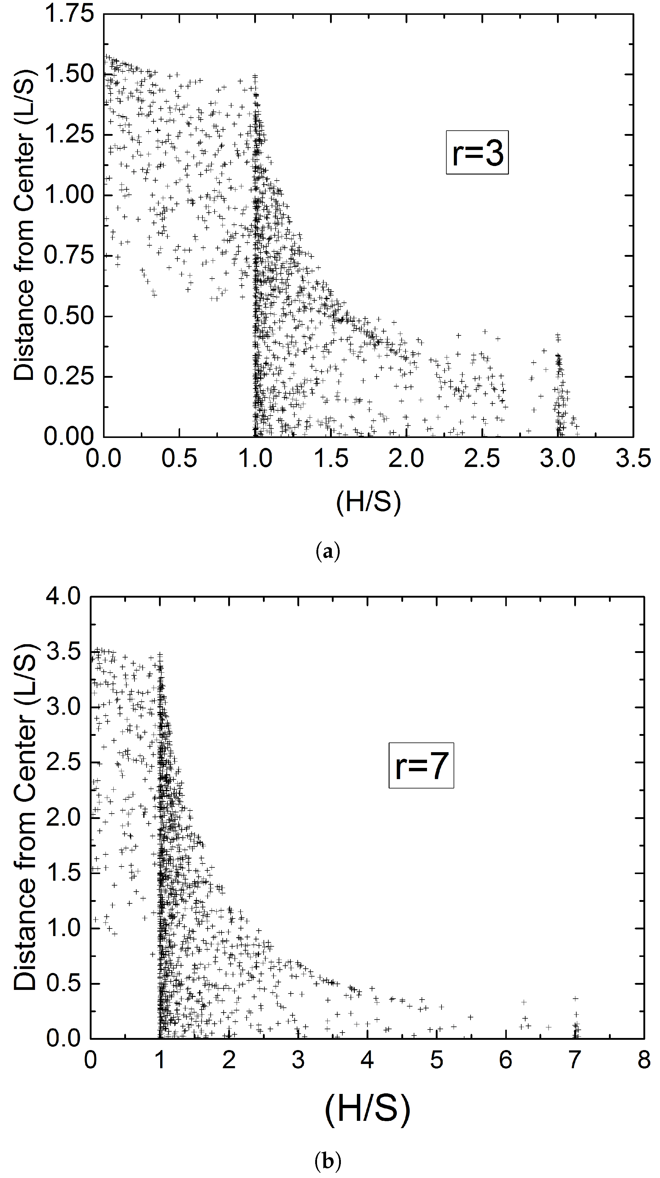
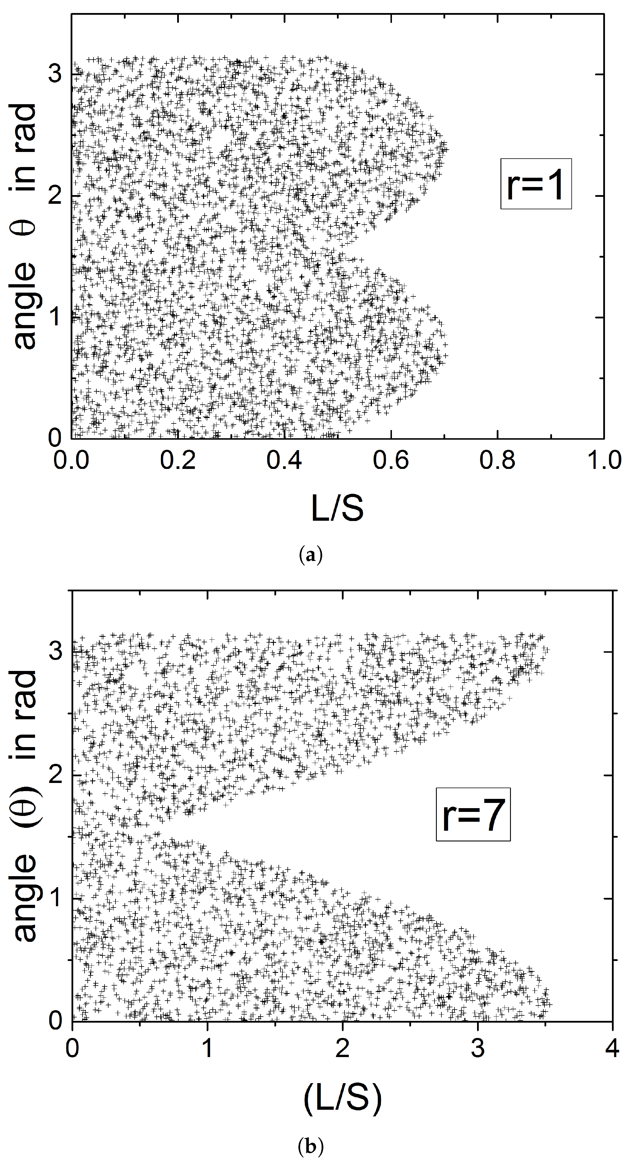
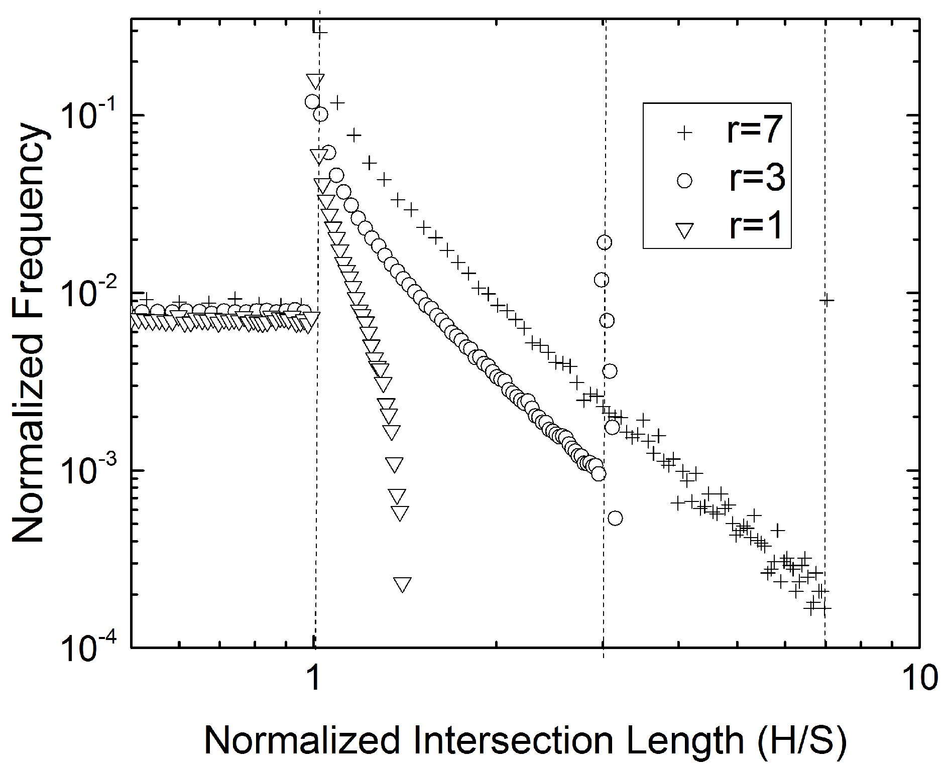
4.1. General Observations
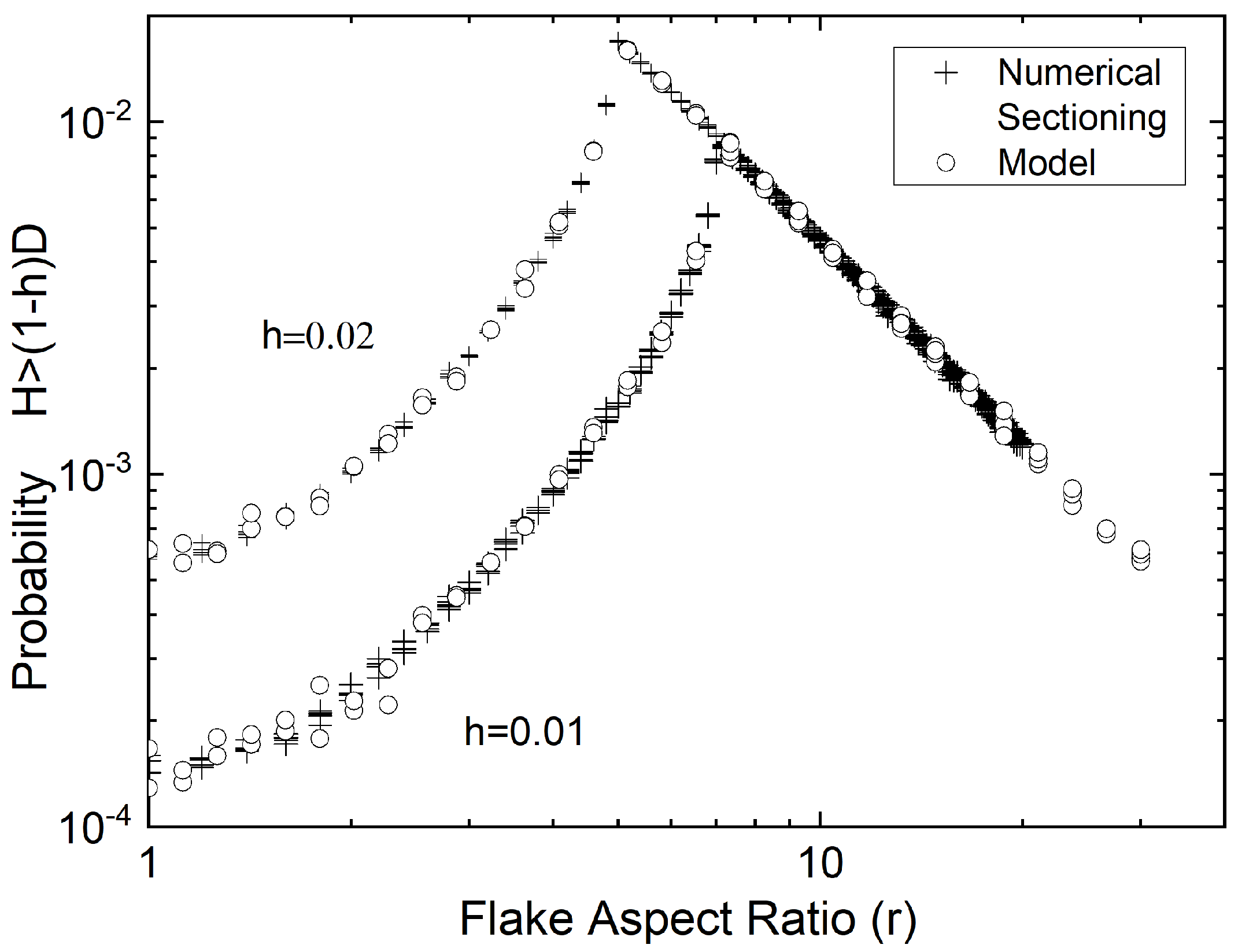
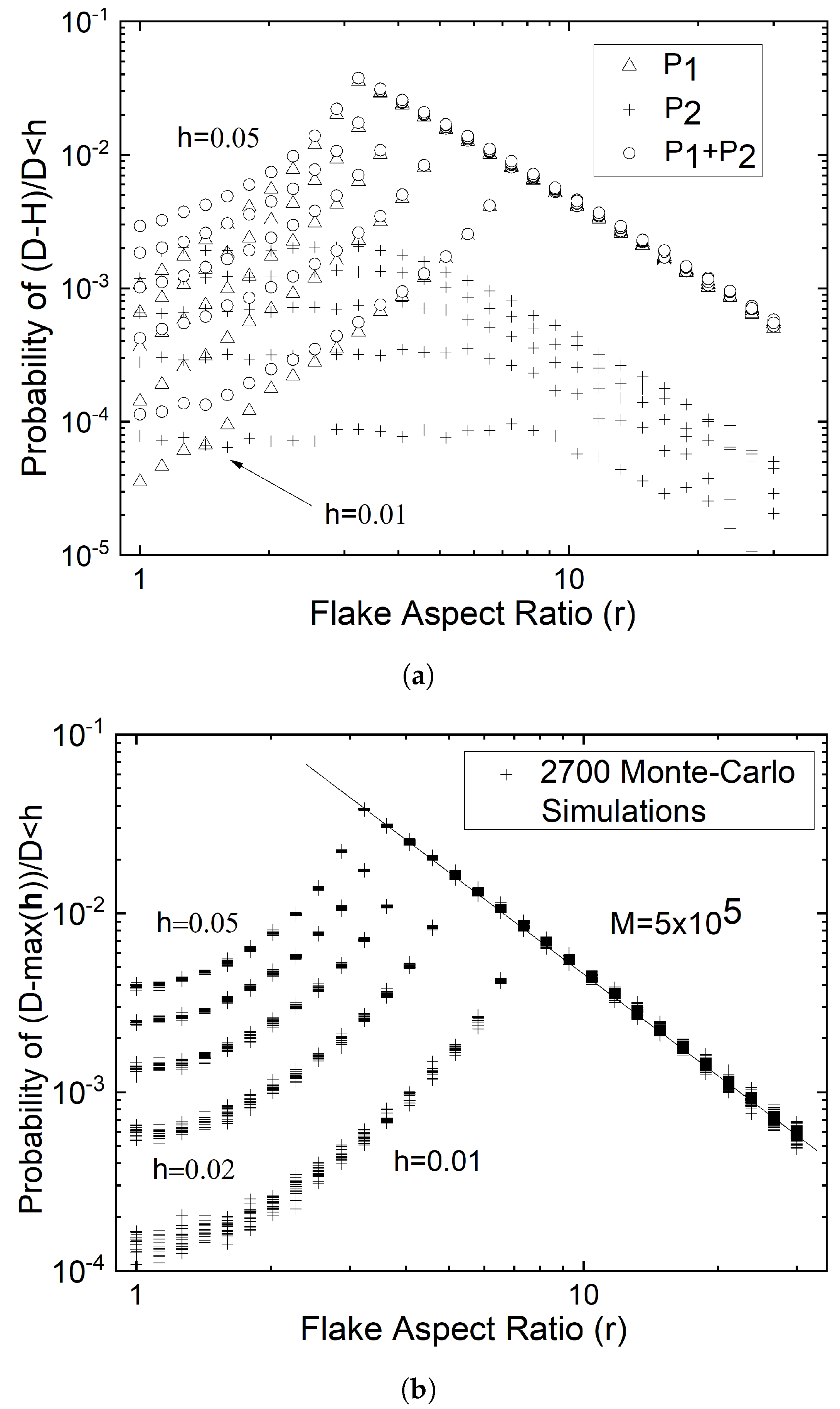
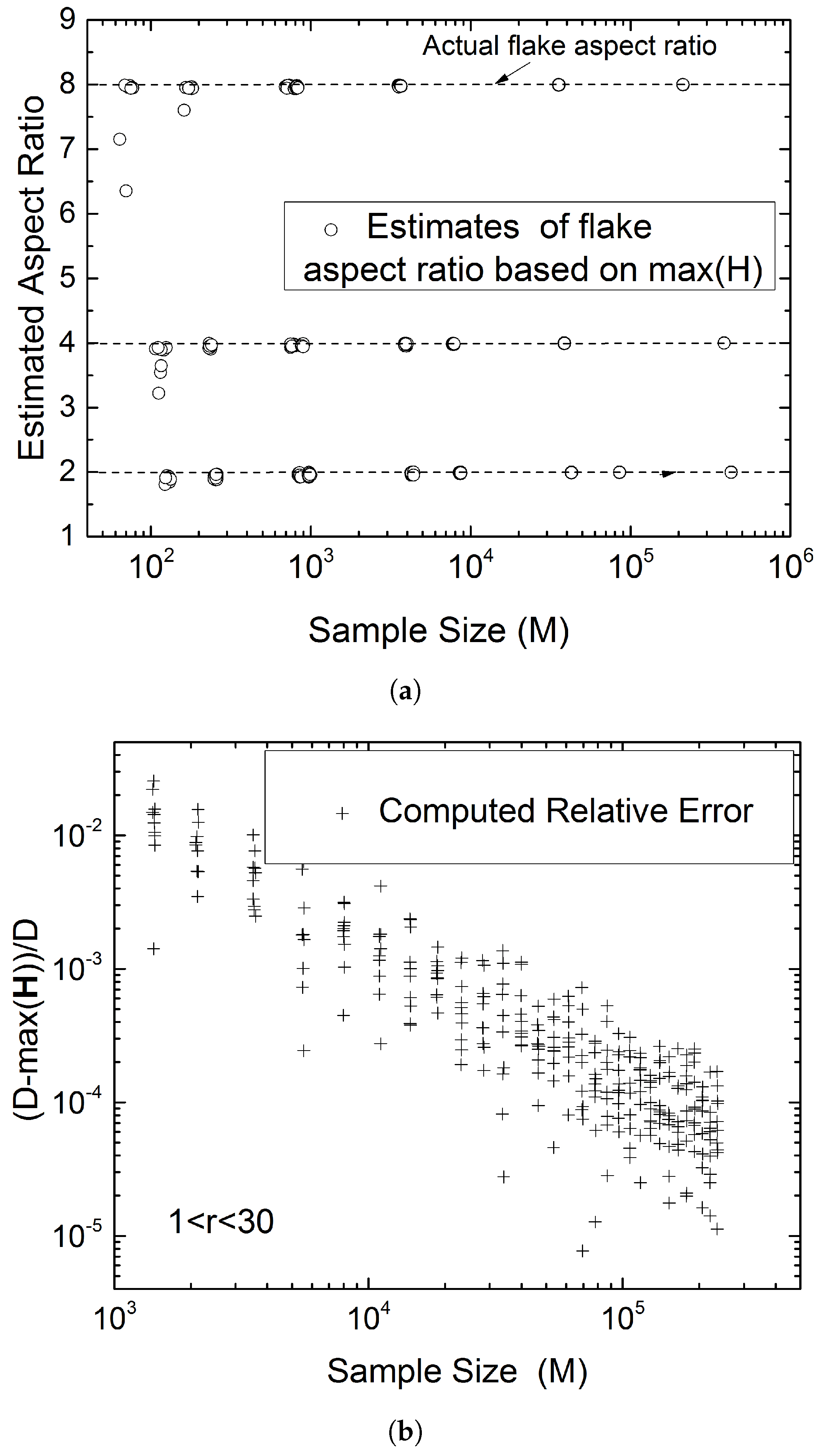
4.2. Determination of the Flake Aspect Ratio from the Maximum Intersection Length
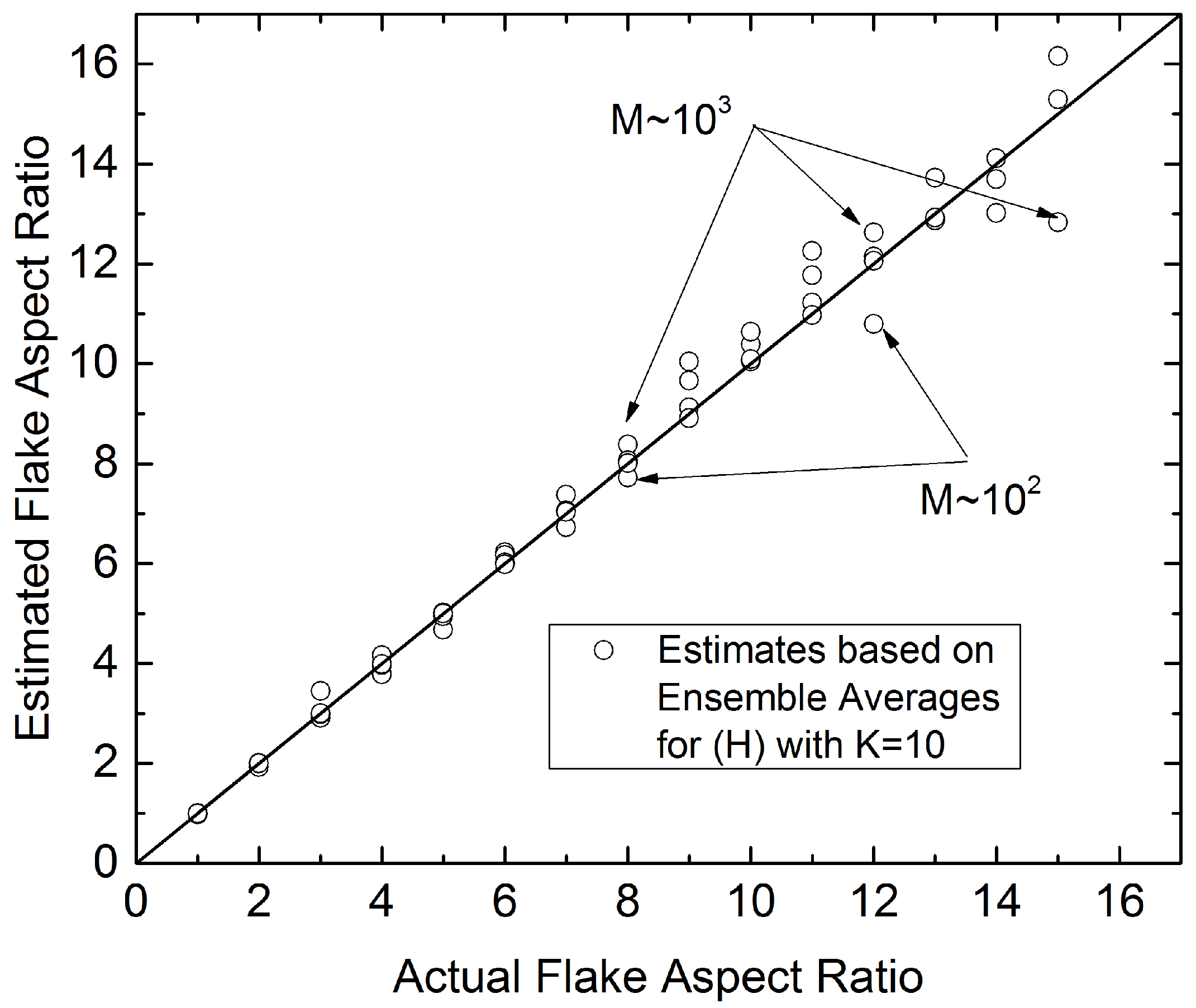
4.3. Determination of Flake Aspect Ratio from the Average of the Intersection Lengths
4.4. Comparison between Predictions and Results of Numerical Experiments
5. Conclusions
Author Contributions
Funding
Data Availability Statement
Acknowledgments
Conflicts of Interest
Abbreviations
| 2D | two-dimensional |
| 3D | three-dimensional |
| AFM | Atomic Force Microscopy |
| BIF | Barrier Improvement Factor |
| EMI | Electromagnetic Interference |
| RSA | Random Sequential Addition |
| RVE | Representative Volume Element |
| TEM | Transmission Electron Microscopes |
References
- Clarke, A.; Davidson, N.; Archenhold, G. Mesostructural characterisation of aligned fibre composites. In Flow-Induced Alignment in Composite Materials; Elsevier: Amsterdam, The Netherlands, 1997; pp. 230–292. [Google Scholar]
- Da Costa, J.P.; Oprean, S.; Baylou, P.; Germain, C. Stereological estimation of orientation distribution of generalized cylinders from a unique 2D slice. Microsc. Microanal. 2013, 19, 1678–1687. [Google Scholar] [CrossRef] [Green Version]
- Clarke, A.; Eberhardt, C. The representation of reinforcing fibres in composites as 3D space curves. Compos. Sci. Technol. 1999, 59, 1227–1237. [Google Scholar] [CrossRef]
- Eberhardt, C.; Clarke, A.; Vincent, M.; Giroud, T.; Flouret, S. Fibre-orientation measurements in short-glass-fibre composites—II: A quantitative error estimate of the 2d image analysis technique. Compos. Sci. Technol. 2001, 61, 1961–1974. [Google Scholar] [CrossRef]
- Bale, H.; Blacklock, M.; Begley, M.R.; Marshall, D.B.; Cox, B.N.; Ritchie, R.O. Characterizing three-dimensional textile ceramic composites using synchrotron X-ray micro-computed-tomography. J. Am. Ceram. Soc. 2012, 95, 392–402. [Google Scholar] [CrossRef]
- Lee, Y.; Lee, S.; Youn, J.; Chung, K.; Kang, T. Characterization of fiber orientation in short fiber reinforced composites with an image processing technique. Mater. Res. Innov. 2002, 6, 65–72. [Google Scholar] [CrossRef]
- Martín-Herrero, J.; Germain, C. Microstructure reconstruction of fibrous C/C composites from X-ray microtomography. Carbon 2007, 45, 1242–1253. [Google Scholar] [CrossRef] [Green Version]
- Nyflött, Å.; Meriçer, Ç.; Minelli, M.; Moons, E.; Järnström, L.; Lestelius, M.; Baschetti, M.G. The influence of moisture content on the polymer structure of polyvinyl alcohol in dispersion barrier coatings and its effect on the mass transport of oxygen. J. Coat. Technol. Res. 2017, 14, 1345–1355. [Google Scholar] [CrossRef]
- Xia, L.; Wu, H.; Guo, S.; Sun, X.; Liang, W. Enhanced sound insulation and mechanical properties of LDPE/mica composites through multilayered distribution and orientation of the mica. Compos. Part A Appl. Sci. Manuf. 2016, 81, 225–233. [Google Scholar] [CrossRef]
- Dasari, A.; Yu, Z.Z.; Cai, G.P.; Mai, Y.W. Recent developments in the fire retardancy of polymeric materials. Prog. Polym. Sci. 2013, 38, 1357–1387. [Google Scholar] [CrossRef]
- Kortschot, M.; Woodhams, R. Computer simulation of the electrical conductivity of polymer composites containing metallic fillers. Polym. Compos. 1988, 9, 60–71. [Google Scholar] [CrossRef]
- Taherian, R. Experimental and analytical model for the electrical conductivity of polymer-based nanocomposites. Compos. Sci. Technol. 2016, 123, 17–31. [Google Scholar] [CrossRef]
- Kandasubramanian, B.; Gilbert, M. An electroconductive filler for shielding plastics. In Macromolecular Symposia; Wiley Online Library: Weinheim, Germany, 2005; Volume 221, pp. 185–196. [Google Scholar]
- Jiang, G.; Gilbert, M.; Hitt, D.; Wilcox, G.; Balasubramanian, K. Preparation of nickel coated mica as a conductive filler. Compos. Part A Appl. Sci. Manuf. 2002, 33, 745–751. [Google Scholar] [CrossRef]
- Tsiantis, A.; Papathanasiou, T.D. A general scaling for the barrier factor of composites containing thin layered flakes of rectangular, circular and hexagonal shape. Int. J. Heat Mass Transf. 2020, 157, 119962. [Google Scholar] [CrossRef]
- Tsiantis, A.; Wang, Y.; Huang, X.; Papathanasiou, T.D. From flakes to ribbons: The barrier factor of composites containing flakes of rectangular shape. J. Compos. Mater. 2022, 56, 181–198. [Google Scholar] [CrossRef]
- Meunier, J.L.; Mendoza-Gonzalez, N.Y.; Pristavita, R.; Binny, D.; Berk, D. Two-dimensional geometry control of graphene nanoflakes produced by thermal plasma for catalyst applications. Plasma Chem. Plasma Process. 2014, 34, 505–521. [Google Scholar] [CrossRef]
- Lin, L.S.; Bin-Tay, W.; Li, Y.R.; Aslam, Z.; Westwood, A.; Brydson, R. A practical characterisation protocol for liquid-phase synthesised heterogeneous graphene. Carbon 2020, 167, 307–321. [Google Scholar] [CrossRef]
- Jiang, J.; Wong, C.P.Y.; Zou, J.; Li, S.; Wang, Q.; Chen, J.; Qi, D.; Wang, H.; Eda, G.; Chua, D.H.; et al. Two-step fabrication of single-layer rectangular SnSe flakes. 2D Mater. 2017, 4, 021026. [Google Scholar] [CrossRef]
- Zeng, X.; Hirwa, H.; Ortel, M.; Nerl, H.C.; Nicolosi, V.; Wagner, V. Growth of large sized two-dimensional MoS 2 flakes in aqueous solution. Nanoscale 2017, 9, 6575–6580. [Google Scholar] [CrossRef]
- Peng, Y.Y.; Akuzum, B.; Kurra, N.; Zhao, M.Q.; Alhabeb, M.; Anasori, B.; Kumbur, E.C.; Alshareef, H.N.; Ger, M.D.; Gogotsi, Y. All-MXene (2D titanium carbide) solid-state microsupercapacitors for on-chip energy storage. Energy Environ. Sci. 2016, 9, 2847–2854. [Google Scholar] [CrossRef] [Green Version]
- Mag-isa, A.E.; Kim, J.H.; Lee, H.J.; Oh, C.S. A systematic exfoliation technique for isolating large and pristine samples of 2D materials. 2D Mater. 2015, 2, 034017. [Google Scholar] [CrossRef]
- Santos, J.C.; Prado, M.C.; Morais, H.L.; Sousa, S.M.; Silva-Pinto, E.; Cançado, L.G.; Neves, B.R. Topological vectors as a fingerprinting system for 2D-material flake distributions. npj 2D Mater. Appl. 2021, 5, 51. [Google Scholar] [CrossRef]
- Decker, J.J.; Meyers, K.P.; Paul, D.R.; Schiraldi, D.A.; Hiltner, A.; Nazarenko, S. Polyethylene-based nanocomposites containing organoclay: A new approach to enhance gas barrier via multilayer coextrusion and interdiffusion. Polymer 2015, 61, 42–54. [Google Scholar] [CrossRef]
- Spencer, M.W.; Hunter, D.; Knesek, B.; Paul, D. Morphology and properties of polypropylene nanocomposites based on a silanized organoclay. Polymer 2011, 52, 5369–5377. [Google Scholar] [CrossRef]
- Zhang, D.; Zhan, Z. Strengthening effect of graphene derivatives in copper matrix composites. J. Alloys Compd. 2016, 654, 226–233. [Google Scholar] [CrossRef]
- Adak, B.; Joshi, M.; Butola, B.S. Polyurethane/clay nanocomposites with improved helium gas barrier and mechanical properties: Direct versus master-batch melt mixing route. J. Appl. Polym. Sci. 2018, 135, 46422. [Google Scholar] [CrossRef]
- Tsiantis, A.; Papathanasiou, T.D. A novel FastRSA algorithm: Statistical properties and evolution of microstructure. Phys. A Stat. Mech. Its Appl. 2019, 534, 122083. [Google Scholar] [CrossRef]
- Lim, I.L.H.; Yang, D. Low-cost precision motion control for industrial digital microscopy. In Proceedings of the IECON 2017—43rd Annual Conference of the IEEE Industrial Electronics Society, Beijing, China, 29 October–1 November 2017; pp. 7281–7287. [Google Scholar]
- Merchant, F.A.; Castleman, K.R. Computer-assisted microscopy. In The Essential Guide to Image Processing; Elsevier: Amsterdam, The Netherlands, 2009; pp. 777–831. [Google Scholar]
- Barwick, S.C.; Papathanasiou, T.D. Identification of sample preparation defects in automated topological characterization of composite materials. J. Reinf. Plast. Compos. 2003, 22, 655–669. [Google Scholar] [CrossRef]
- Barwick, S.C.; Papathanasiou, T.D. Identification of fiber misalignment in continuous fiber composites. Polym. Compos. 2003, 24, 475–486. [Google Scholar] [CrossRef]
- Davidson, N.; Clarke, A. Extending the dynamic range of fibre length and fibre aspect ratios by automated image analysis. J. Microsc. 1999, 196, 266–272. [Google Scholar] [CrossRef]
- Leroy, M.; Acher, O. Assessment of microscopy moving stage performance down to the 10 nm range using encoded patterns with automated reading. In Proceedings of the Euspen 18th International Conference & Exhibition, Venise, Italy, 4–8 June 2018. [Google Scholar]


| M | |||||||
|---|---|---|---|---|---|---|---|
| 1 | 1 | 130 | 0.7772 | 0.03429 | 0.025857 | 0.979 | 0.06451 |
| 1250 | 0.7866 | 0.00765 | 0.005773 | 1.003 | 0.01475 | ||
| 12,500 | 0.7851 | 0.00324 | 0.002443 | 0.999 | 0.00622 | ||
| 128,000 | 0.7849 | 0.00071 | 0.000533 | 0.999 | 0.00135 | ||
| 1 | 2 | 125 | 1.0331 | 0.04439 | 0.033471 | 1.922 | 0.18200 |
| 1230 | 1.0474 | 0.01480 | 0.011162 | 2.002 | 0.06405 | ||
| 12,350 | 1.0481 | 0.00487 | 0.003671 | 2.006 | 0.02112 | ||
| 127,000 | 1.0471 | 0.00106 | 0.000804 | 2.000 | 0.00461 | ||
| 1 | 3 | 120 | 1.2179 | 0.04845 | 0.036532 | 3.453 | 0.46120 |
| 1180 | 1.1691 | 0.00857 | 0.00646 | 2.912 | 0.06293 | ||
| 12,080 | 1.1763 | 0.00542 | 0.004087 | 2.983 | 0.04128 | ||
| 121,000 | 1.1780 | 0.00222 | 0.001675 | 3.000 | 0.01707 | ||
| 1 | 4 | 115 | 1.2419 | 0.04515 | 0.034041 | 3.779 | 0.49493 |
| 1130 | 1.2663 | 0.03251 | 0.024512 | 4.161 | 0.41566 | ||
| 11,500 | 1.2548 | 0.00430 | 0.003242 | 3.973 | 0.05105 | ||
| 116,000 | 1.2558 | 0.00241 | 0.001818 | 3.989 | 0.02882 | ||
| 1 | 5 | 110 | 1.2936 | 0.06103 | 0.046016 | 4.671 | 0.94229 |
| 1120 | 1.3063 | 0.02227 | 0.016791 | 4.943 | 0.37765 | ||
| 11,500 | 1.3097 | 0.00739 | 0.005576 | 5.021 | 0.12870 | ||
| 116,000 | 1.3090 | 0.00249 | 0.001876 | 5.003 | 0.04305 | ||
| 1 | 6 | 105 | 1.3531 | 0.08089 | 0.060993 | 6.222 | 202.580 |
| 1070 | 1.3516 | 0.01873 | 0.014119 | 6.171 | 0.46234 | ||
| 11,000 | 1.3468 | 0.01087 | 0.008198 | 6.017 | 0.25705 | ||
| 110,000 | 1.3459 | 0.00195 | 0.001473 | 5.989 | 0.04581 | ||
| 1 | 8 | 105 | 1.3905 | 0.10717 | 0.080805 | 7.723 | 391.494 |
| 1060 | 1.4032 | 0.03815 | 0.028768 | 8.383 | 161.267 | ||
| 10,550 | 1.3974 | 0.00511 | 0.003852 | 8.067 | 0.20164 | ||
| 105,000 | 1.3963 | 0.00251 | 0.001892 | 8.012 | 0.09783 | ||
| 1 | 12 | 105 | 1.4375 | 0.09517 | 0.071758 | 10.80 | 636.127 |
| 1070 | 1.4553 | 0.03430 | 0.025864 | 12.62 | 30.565 | ||
| 11,000 | 1.4511 | 0.01171 | 0.008827 | 12.14 | 0.97103 | ||
| 103,000 | 1.4503 | 0.00304 | 0.00229 | 12.06 | 0.24868 | ||
| 1 | 15 | 1030 | 1.4571 | 0.02617 | 0.019735 | 12.83 | 240.496 |
| 10,600 | 1.4790 | 0.00762 | 0.005747 | 16.16 | 107.709 | ||
| 101,000 | 1.4742 | 0.00548 | 0.004137 | 15.29 | 0.69910 |
Publisher’s Note: MDPI stays neutral with regard to jurisdictional claims in published maps and institutional affiliations. |
© 2022 by the authors. Licensee MDPI, Basel, Switzerland. This article is an open access article distributed under the terms and conditions of the Creative Commons Attribution (CC BY) license (https://creativecommons.org/licenses/by/4.0/).
Share and Cite
Papathanasiou, T.D.; Tsiantis, A.; Wang, Y. A Novel Method for the Determination of the Lateral Dimensions of 2D Rectangular Flakes. Materials 2022, 15, 1560. https://doi.org/10.3390/ma15041560
Papathanasiou TD, Tsiantis A, Wang Y. A Novel Method for the Determination of the Lateral Dimensions of 2D Rectangular Flakes. Materials. 2022; 15(4):1560. https://doi.org/10.3390/ma15041560
Chicago/Turabian StylePapathanasiou, Thanasis D., Andreas Tsiantis, and Yanwei Wang. 2022. "A Novel Method for the Determination of the Lateral Dimensions of 2D Rectangular Flakes" Materials 15, no. 4: 1560. https://doi.org/10.3390/ma15041560
APA StylePapathanasiou, T. D., Tsiantis, A., & Wang, Y. (2022). A Novel Method for the Determination of the Lateral Dimensions of 2D Rectangular Flakes. Materials, 15(4), 1560. https://doi.org/10.3390/ma15041560