Abstract
This study was devoted to an investigation on the dynamics of double-walled carbon nanotubes (DWCNTs) under the influence of Winkler–Pasternak foundation near the primary resonance. Two Euler–Bernoulli beams embedded on nonlinear foundation, interacting through van der Waals forces, subjected to mechanical impact are considered. By means of Hamilton’s principle, Eringen’s nonlocal elastic theory, and taking into account the moving nanoparticles, the Galerkin–Bubnov method is applied and accordingly, governing partial differential equations are reduced to two differential equations with variable coefficients. The nonlinear damped and forced vibration is studied using the optimal auxiliary functions method (OAFM). An explicit and very accurate analytical solution is obtained by means of OAFM without considering simplifying hypotheses. An accurate analysis is for the first time reported considering the cumulated effects of nonlinearities simultaneously induced by the Winkler–Pasternak foundation, the curvature of beams and van der Waals force, and also the effect of discontinuities marked by the presence of the Dirac function. Finally, a stability analysis of the considered model is developed by means of the homotopy perturbation method (HPM) using the condition of existence of the two frequencies. It was shown that an increasing of some constitutive parameters substantially reduces the area of stability, all these being of much help in guiding the design of advanced nanoelectromechanical devices, in which nanotubes act as basic elements.
1. Introduction
Starting with the discovery of carbon nanotubes (CNTs) by Iijima [1] in 1991, much research has been conducted on this new attractive topic in the field of nanotechnology. CNTs have a lot of applications in atomic-force microscopy, gas storage, fluid transport, nanosprings, nanofillers, nanomotors, agricultural or chemical industry, nanoelectromechanical devices, fuel cells, thermal and electrical conductivities, and so on. Slender or functionally graded Euler–Bernoulli, Timoshenko, Reddy, or Rayleigh beams, linear or nonlinear with Pasternak or Winkler foundation with or without van der Waals interactions, and free or forced vibrations were investigated in the last few years. These studies were basically conducted in two different principal ways delimited by considering or not the nonlinearity and associated nonlinear effects. In the first approach, nonlinearity and nonlinear terms were omitted, and in this first category of studies, a closed-form solution for the vibration of a linear carbon chain in CNTs was derived by Ding et al. [2] by means of continuum modeling of the van der Waals interactions. Analytical results showed that the vibration frequency of the carbon chain in a (5,5) CNT could be around two orders of magnitude higher than that of an independent carbon chain without initial tensile force. Rezapour and Araghi [3] considered the effects of inertia and Coriolis forces due to nanoparticle movement and viscoelastic behavior of single-walled carbon nanotubes (SWCNTs) is established by the Kelvin–Voigt viscoelastic model. The dynamic amplitude was found in this study almost 30% higher than the corresponding value obtained from the moving load model. The incremental harmonic balance method was implemented by Pirmoradian et al. [4] to investigate the parametric resonance of double-walled carbon nanotubes (DWCNTs) loaded by successive nanoparticles through the drug-delivery process. Comparing the static tensile axial force with the case of compressive force, they concluded that the DWCNT is more stable in the first case. Moreover, the instability of transverse vibration of an embedded DWCNT for the delivery of successive nanoparticles was investigated by Pirmoradian et al. [5] considering the van der Waals force and inertial effects of moving nanoparticles, and stability was determined by the incremental harmonic balance method.
A more realistic approach closer to the reality is obtained by considering also the nonlinearity in modeling these kinds of problems. Such nonlinear models were investigated by different researchers using various analytical techniques applicable in analyzing nonlinear differential equations. Soltani and Farshidianfar [6] applied the energy balance method in the study of vibrations of SWCNTs embedded on Pasternak-type foundation. The results showed that the nonlinearity can be tuned by applying axial tension to the nanotube. Khosrozadeh and Hajabasi [7] used the harmonic balance method for nonlinear free vibration of DWCNTs based on Euler–Bernoulli beam theory modeled by van der Waals force. The same procedure was applied by Fang et al. [8] for free vibration of clamped–clamped DWCNTs taking into account von Karman geometric nonlinearity, showing that the amplitudes of vibration in the case of van der Waals forces are larger than those considering both geometric nonlinearity and van der Waals force. Arani et al. [9] investigated single-walled boron nitride nanotubes (SWBNNTs) by means of the method of multiple scales and of differential quadrature. The interaction between the inner viscous fluid and SWBNNTs was studied by means of Navier–Stokes equations decoupling the electrical and mechanical fields. The parametrized perturbation method was proposed by Valipour et al. [10] to characterize the nonlinear vibration of embedded SWCNTs conveying fluid, employing Pasternak-type elastic foundation. The result is that by increasing the Winkler constant, the nonlinear frequency decreases. A modified variational iteration method was proposed by Pashaki and Li [11] to study strongly nonlinear vibration of CNTs conveying viscous fluid, which is a damped vibrational system. The results showed that with an increase in amplitude and incorporating the geometric nonlinearity, the effect of the viscosity became more apparent. Miashiro et al. [12] explored the mechanical vibration of SWCNTs at different lengths and carbon nanobelt forms with beam elements, showing that SWCNTs and carbon nanobelts smaller than the aspect ratio 1 significantly increase the static modulus and their first vibration mode also changes from bending mode to the radial mode. By using Fourier-transform infrared spectroscopy, Line et al. [13] employed the impacts of CNTs and titanium dioxide nanoparticles on tomato plants after a number of days of exposure in soil. They established modifications in leaf cell wall components of plants. Civalek et al. [14] analyzed the free vibration behavior of carbon nanotube-reinforced composite microbeams. CNTs are distributed in a polymeric matrix with four patterns of the reinforcement and the material properties are predicted by the rule of mixture T. The free vibration of a tapered beam modeling nonuniform SWCNT i.e., nanocones, was studied by De Rosa et al. [15] using the differential quadrature method applied to compute the natural frequencies for the clamped beam at one end and elastically restrained at the other. Su and Cho [16] examined the influences of the slenderness ratios, the boundary conditions, the atomic structures and the stiffness of the embedded medium on the natural frequencies and mode shapes of SWCNTs on the basis of the nonlocal cantilever Timoshenko beam model. Senthilkumar [17] studied the axial vibration of DWCNTs without decoupling the continuum model by means of the semianalytical procedure. The Pasternak medium support and magnetic effects influence the frequencies of the first and the second nanotubes. Hossain and Lellep [18] presented the Maclaurin series approach to solve the equation of motion derived from the Euler–Bernoulli beam theory based on Eringen’s nonlocal theory of elasticity. Accordingly, the upper beam influences the mode shape of the upper beams as well as the intact lower beam. Chen et al. [19] investigated the forced vibrations of a functionally graded double-nanobeam system on an elastic foundation using Eringen’s nonlocal elasticity theory. The explicit expressions of the stationary responses were obtained by Green’s functions method in conjunction with the superposition principle, leading to the conclusion that the bond between the two nanobeams can be significantly reinforced by increasing the stiffness and damping coefficient of the connecting layer.
Different practical applications of CNTs in various devices and materials or structures were recently reported [20,21,22,23], emphasizing their usefulness and efficiency. Baydin et al. [20] presented a comprehensive review of the current developments in the field of carbon nanotube devices for quantum technology, discussing recent progress in the development of carbon-nanotube-based devices and strategies for revolutionizing computation, sensing, and communication as components of quantum technology. Oh et al. [21] proposed an application of carbon nanotubes (CNTs), a conductive carbon nanofiller, and polydimethylsiloxane as a polymer matrix, to fabricate a flexible pressure sensor, and its piezoresistive and capacitive pressure-sensing characteristics were deeply analyzed, emphasizing a great potential for practical applications in manufacturing pressure sensors. Merodio-Perea et al. [22] studied the mechanical properties of cement reinforced with pristine and functionalized carbon nanotubes, showing that the incorporation of CNTs enhances the mechanical properties of tobermorite as a consequence of better interactions that are established at the cement–CNT interface. Páez-Pavón et al. [23] reported interesting results of the addition of different types of carbon nanotubes on the microstructure and on the physical properties of cement paste. The microstructure was analyzed and the electrical conductivity for different CNT concentrations was measured, identifying improved features of great interest in the field of construction materials.
In the present study, we investigated the nonlinear forced vibration of DWCNTs subjected to mechanical impact and embedded on Winkler–Pasternak foundation in the neighborhood of the primary resonance. Two Euler–Bernoulli beams interacting through van der Waals forces are considered in the paper. Using the Hamilton principle and Eringen’s nonlocal elastic theory, taking into consideration the moving nanoparticles, we obtain two partial differential equations as governing equations, which are reduced by means of the Galerkin–Bubnov procedure to two differential equations with variable coefficients. For the first time, we considered the cumulated effects of nonlinearities induced by the Winkler–Pasternak foundation, the curvature of beams and the nonlinear van der Waals force, and also the effect of discontinuities marked by the presence of the Dirac function. The nonlinear differential equations are studied by means of the optimal auxiliary functions method (OAFM). An explicit and very accurate analytical approximate solution is obtained using the so-called auxiliary functions and a moderate number of convergence-control parameters, independently of the presence of small or large parameters in the governing equations or in the boundary/initial conditions. Finally, a stability analysis of the considered model is developed by means of the homotopy perturbation method (HPM) using the condition of existence of the two frequencies, which led to the establishment of the borderline cases, all these being of much help in guiding the design of advanced nanoelectromechanical devices, in which nanotubes act as basic elements.
2. Governing Equations
In Figure 1 is depicted a double tube of length l, having inner radius R1, outer radius R2, Young’s modulus E and density ρ.
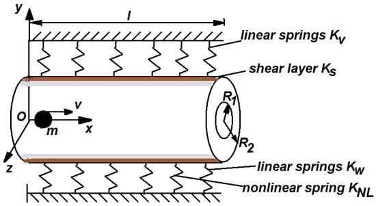
Figure 1.
Geometry of DWCNT on Winkler–Pasternak foundation under the moving nanoparticle.
The Winkler–Pasternak foundation is characterized by shear layer constant Ks, the linear spring Kw and nonlinear spring KNL. Through inner tube moves the nanoparticle of mass m and with constant speed v. While the nanoparticle arrives at the right end, another nanoparticle moves immediately. Simply supported boundary conditions are assumed. The extended Hamilton principle for a system with changing mass and based on Euler–Bernoulli beam theory can be written as
where T, Π and WNP are kinetic energy, potential energy (which include the strain energy of nanotube, potential energy from Winkler–Pasternak foundation and potential energy due to van der Waals forces) and the work done by the moving nanoparticle m, respectively. The Euler–Bernoulli theory supposes that the vector perpendicular to the neutral axis x of the beam remains perpendicular after deformation and accordingly, the deformation due to shear stress is neglected. Also, the longitudinal displacement of the beam can be neglected.
The displacement field can be written as [4,5,7,8]:
where , , are the displacements of an arbitrary point along x-, y-, z- directions, respectively. For small deflection, the strain component is
Hooke’s law for linear deformations becomes:
The kinetic energy of DWCNT is
where A1 and A2 are cross-sections of the inner and outer tubes, respectively.
The strain energy of nanotubes stored in the DWCNT is
The potential energy derived from Winkler–Pasternak foundation can be written in the form
The potential energy derived from van der Waals forces can be given by
where P12 is the force applied to the outer tube by the inner one and P21 is the force applied to the inner tube by the outer one. In this case it holds that P12 = −P21 = Pv and for the nonlinear analyses the potential of van der Waals forces can be extended by Taylor expansion around the equilibrium points as [9]:
The work done by the moving particle m is
in which F(x,t) is a combination of the loading function with the inertial effect of the moving nanoparticle
where the material derivative of W1 can be expressed as
and g is the gravity acceleration, Kv is the linear spring constant utilized to simulate the van der Waals force between the mass m and the DWCNT, H is the Heaviside function and δ is the Dirac function.
Substituting Equations (11) and (12) into Equation (10), we have:
Substituting Equations (5)–(8) and (13) into Equation (1) and calculating the variation of W1 and W2, the governing equations of motion are:
Based on Eringen’s nonlocal theory [24], the constitutive relations for homogeneous isotropic beams can be approximated by using Green’s function as [5]:
From the last equation, after it is multiplied by z and then is integrated, the nonlocal stress resultant becomes:
where we used the relation
Using the approximation
and performing some manipulations, from Equations (14), (15), (17) and (19), the governing equations of motion are:
In order to discretize the Equations (20) and (21), by applying the Galerkin–Bubnov procedure, the displacement of the DWCNT for the simply supported case are given by
Substituting Equation (22) into Equations (20) and (21), multiplying then by and integrating over the domain [0,l], one gets:
By means of non-dimensional parameters
the governing Equations (23) and (24) can be written as
where the prime denotes differentiation with respect to τ*.
The initial conditions for Equations (26) and (27) are
Equations (26)–(28) are second-order nonlinear differential equations with variable coefficients, and therefore are very difficult to be analytically solved. In what follows, for Equations (26)–(28), the OAFM is applied to study the nonlinear vibration near the primary resonance.
3. Basics of the Optimal Auxiliary Functions Methods
For a general nonlinear differential equation [25,26,27,28,29,30,31]
with the initial conditions
where L is a linear operator, N is a nonlinear operator, D is the domain of interest, B is a boundary operator, we propose that the approximate solution to be of the form
where Ci are n parameters unknown at this moment and n is an arbitrary positive integer number. The initial approximation Q0(τ) can be determined from the linear differential equation
with the initial conditions
Taking into consideration the last two equations, the first approximation Q1(τ,Ci) is obtained from the nonlinear differential equation
with the initial conditions
However, the nonlinear differential Equations (34) and (35) are very difficult to solve. We propose the following alternative. The nonlinear term of Equation (34) is developed in the form
where k! = 1, 2, …, k and N(k) denotes differentiation of order k of the nonlinear operator N. To avoid the difficulties that appear in solving the nonlinear differential Equation (36), and to accelerate the convergence of the first approximate solution Q1, instead of solving the following equation obtained from Equations (34) and (36):
we make the fundamental remarks as follows. In general, the solution of liner differential Equations (32) and (33) is known and can be expressed in the form
where the coefficients ai, the functions fi(τ) and integer positive p are known. Now, the nonlinear operator N[Q0(τ)] calculated for Q0(τ) given by Equation (38), may be written as
where the coefficients bj, the functions gi(τ) and positive integer q are known and depend on the initial approximation Q0(τ) and also on the nonlinear operator N. Since Equation (37) is very difficult to solve, according to OAFM procedure, it is more convenient to consider that the first approximation Q1(τ,Ci) can be solution of linear differential equation
where Hj are m < p so-called auxiliary functions which depend on n parameters Ci and can be chosen as mathematical expressions similar with Q0(τ) and N[Q0(τ)]. The functions gj are only m functions involved in Equation (39). In the case of vibration problems, the resonant terms into Equation (40) must be avoided. From this condition, we can obtain the expression of the frequency. After this clarification, the linear Equation (40) can be easily solved.
In consequence, the first approximation is determined from Equation (40) and the approximate solution of Equations (29) and (30) is determined from Equations (31), (32) and (40).
Finally, the unknown parameters Ci, i = 1, 2, …, n can be optimally identified via rigorous mathematical procedures, such as the Galerkin method, least square method, Ritz method, collocation method, Kantorovich method, and so on.
In this way, the optimal values of the convergence-control parameters are known and accordingly, the approximate solution is well-determined. Let us note that the nonlinear differential Equations (29) and (30) are reduced to two linear differential equations. This technique led to a very accurate result, is effective, explicit and provides a rigorous way to control and adjust the convergence of the solutions, without the presence of small parameters.
4. Application of OAFM to the Governing Equations of Nonlinear DWCNT System
If ω1 and ω2 are the frequencies of the tubes, and taking into consideration initial conditions (28), we make the following transformations:
such that Equations (26) and (27) can be rewritten as
The linear and nonlinear operators corresponding to Equations (42) and (43) are respectively
The initial conditions for nonlinear Equations (42) and (43) are
The approximate solutions of Equations (42) and (43) can be written as
The initial approximations X0(τ1) and Y0(τ2) are determined from the following linear differential equations
whose solutions are, respectively,
in which ω1 and ω2 are unknown.
Inserting Equation (48) into the second equations of (43) and (44), we obtain
The auxiliary functions given in Equation (39) corresponding to Equation (50) can be chosen in many forms, such as
or
or
and so on.
The auxiliary functions for Equation (50) can be:
or
or
Having in view only Equations (51) and (54), the first approximations can be obtained from the linear equations
The secular terms that appear in Equations (57) and (58) have to be canceled by equating the coefficients to zero. This leads to the equations:
and accordingly, one can get for the case of resonance: d1 ≈ 4, d3 ≈ 4:
From the initial conditions (47) and (49) it holds that
such that
In this way, the approximate solutions of Equations (26)–(28), having in view the transformations (41) can be obtained from Equations (46), (48), (63) and (64):
5. Numerical Example
The efficiency of our procedure can be proved through the following particular case, in which the values of the parameters are
Following the above procedure, the optimal values of the convergence-control parameters are:
Figure 2 and Figure 3 show the comparison between approximate solution (67) and (68) of nonlinear problems (26)–(28) and numerical solution obtained by means of a fourth-order Runge–Kutta approach.
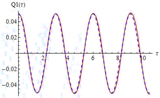
Figure 2.
Comparison between the analytical solution (65) and numerical integration results for Equation (26): red solid line depicts numerical integration results while blue dashed line depicts analytical results.
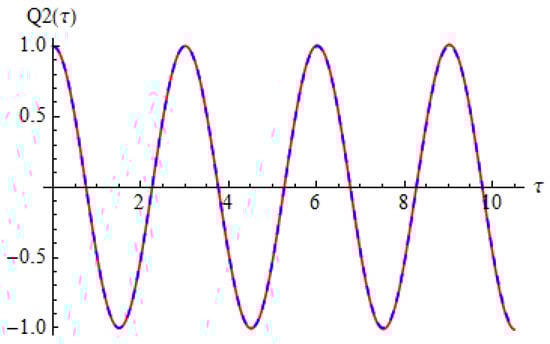
Figure 3.
Comparison between the analytical solution (66) and numerical integration results for Equation (27): red solid line depicts numerical integration results while blue dashed line depicts analytical results.
It can be seen that the two solutions obtained by means of OAFM are nearly identical to the numerical integration results.
6. Stability Analysis
The dynamic behavior of the DWCNT system considering mechanical impact and embedded on Winkler–Pasternak foundation is investigated through homotopy perturbation method [32]. This approach predicts limits of instability in the case of primary resonance . The characteristic of this technique is the presence of an embedding parameter p [0,1] such that for p = 0 any nonlinear differential equation reduces to a linear differential equation and for p = 1 one obtains the original equations. The original Equations (26) and (27) are rewritten omitting the bars and stars as:
We substitute the solution (Q1, Q2) and the coefficients d1 and d3 by the following power series of p:
where Ai and Bi are the solutions of the i-th order homotopy equations, Ω1 and Ω2 are the response frequencies, λi and γi are the i-th coefficients of the expansions.
By substituting Equation (71) into the homotopy Equations (69) and (70) and then identifying the coefficients of the same powers, it results a set two linear differential equations. From these linear equations, secular terms are collected and accordingly the values of the coefficients λi and γi are identified. Each function Ai and Bi are determined separately. Substituting the values of λi and γi into Equation (71), it suffices to replace p = 1 to obtain the frequency Ω1 and Ω2:
In the case in which the expressions below the radical of Equation (72) become zero, then we can obtain the boundaries curve separating regions of stability and instability.
By means of Equation (71), the Equations (69) and (70) can be rewritten using only three terms as:
The initial conditions of Equations (69) and (70) and corresponding Equations (73) and (74) are:
The homotopy equations of order pi, i = 0, 1, 2, … and the initial conditions are as follows:
The solutions of Equations (76) and (77) are
Substituting Equation (82) into Equations (78) and (79), and avoiding secular terms we have
The solutions of Equations (78) and (79) are, respectively:
where
and
where
Now, substituting Equations (82), (83) and (87) into Equations (80) and (81) and avoiding secular terms in the two equations, we obtain
Substituting Equations (83), (89) and (90) into Equation (72) one gets a system of two equations with unknown Ω1 and Ω2. This system can be solved numerically.
The stability boundaries obtained up to the p2 order are presented in Figure 4 and Figure 5 for two particular cases, with different quantities. In Figure 4 is presented the stability domain for the case when a1 = 2, a2 = 2.5, e1 = 3, e2 = 3.3, while in Figure 5 is presented the stability domain for the case when a1 = 0.2, a2 = 0.25, e1 = 0.3, e2 = 0.33.
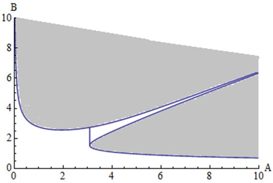
Figure 4.
Stability domain for case 1 (shadow area): a1 = 2, a2 = 2.5, e1 = 3, e2 = 3.3.
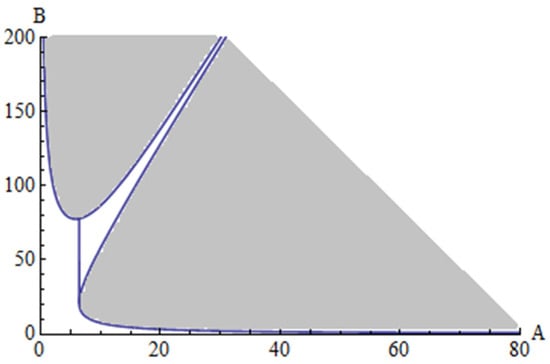
Figure 5.
Stability domain for case 2 (shadow area): a1 = 0.2, a2 = 0.25, e1 = 0.3, e2 = 0.33.
The boundary stability of the first tube is obtained from Equation (72). This boundary curve is , where λ1 and λ2 are given by Equations (83) and (89). On the other hand, the boundary curve of the second tube can be obtained from , where γ1 and γ2 are given by Equations (84) and (90). The area of stability for the first tube is given by and for the second tube the area of stability is given by .
7. Conclusions and Discussion
After carrying out an analysis of nonlinear vibration of double-walled carbon nanotubes subjected to mechanical impact, which is an important research direction in the field of new materials and has a large domain of applicability in engineering practice, the following conclusions can be highlighted.
- We studied the nonlinear vibration of DWCNTs embedded on Winkler–Pasternak foundation, interacting through van der Waals forces, for which the governing differential equations contain nonlinear terms of order three and accordingly such equations are very difficult to solve by exact or approximate methods.
- For the first time is considered the simultaneous presence of nonlinearities induced by the Winkler–Pasternak foundation, the curvature of beams and the nonlinear van der Waals force, and also the effect of discontinuities marked by the presence of the Dirac function, which substantially complicates the governing equations.
- The OAFM was successfully applied to obtain an approximate analytical solution near the primary resonance. In contrast to any other known techniques, the proposed original approach is based on the presence of so-called auxiliary functions and optimal convergence-control parameters which assure high accuracy of the approximate analytical solutions. These parameters are determined by means of rigorous mathematical procedure. The initial and the first iteration are constructed by an original technique and the initial nonlinear governing equations are reduced to only two linear differential equations. Our procedure is easy to apply and very accurate using only the first iteration.
- A numerical example is developed in order to emphasize the accuracy of the proposed analytical solution. In the considered example, it is observed that the variables Q1 and Q2 describing the motion have completely different amplitudes at relatively close frequencies. The amplitude of Q2 is 20 times higher than the amplitude of Q1.
- A stability analysis of the considered model is developed by means of a homotopy perturbation method (HPM) using the condition of existence of the two frequencies of the system. This procedure enables splitting the parameter planes in stable and unstable regions and determines the borderline semianalytically.
- It is observed that an increasing of the values of the constitutive parameters a1, a2, e1, and e2 substantially reduces the area of stability for the considered system. Increasing these values tenfold led to a reduction of approximately 90% of the area of stability.
All the findings emphasized by this research are of important physical significance in guiding the design of advanced devices in the field of nanostructural applications in which nanotubes act as basic elements, with possible applications in nanosensors, nanoresonators, nanoswitches, nanoresistors, nanomotors, nanorobots, and so on.
Author Contributions
Conceptualization, V.M. and N.H.; methodology, V.M.; software, N.H. and B.M.; validation, V.M. and N.H.; formal analysis, V.M.; investigation, V.M., B.M. and N.H.; resources, N.H.; data curation, N.H. and B.M.; writing—original draft preparation, V.M. and N.H.; writing—review and editing, V.M. and N.H.; visualization, N.H. and B.M.; supervision, N.H.; project administration, N.H.; funding acquisition, N.H. All authors have read and agreed to the published version of the manuscript.
Funding
This research received no external funding.
Institutional Review Board Statement
Not applicable.
Informed Consent Statement
Not applicable.
Data Availability Statement
Not applicable.
Conflicts of Interest
The authors declare no conflict of interest.
Abbreviations
| CNTs | carbon nanotubes |
| SWCNTs | single-walled CNTs |
| DWCNTs | double-walled CNTs |
| SWBNNT | single-walled boron nitride nanotubes |
| OAFM | optimal auxiliary functions method |
| HPM | homotopy perturbation method |
References
- Iijima, S. Helical microtubes of graphitic carbon. Nature 1991, 354, 56–58. [Google Scholar] [CrossRef]
- Ding, D.; Zhao, Y.; Dong, S.; Yu, P.; Wang, L.; Zhao, J. The vibration of linear carbon chain in carbon nanotubes. Materials 2017, 10, 478. [Google Scholar] [CrossRef] [PubMed]
- Rezapour, B.; Araghi, M.A.F. Semi-analytical investigation on dynamic response of viscoelastic single-walled carbon nanotube in nanoparticle delivery. J. Brasil. Soc. Mech. Sci. Eng. 2019, 41, 117. [Google Scholar] [CrossRef]
- Pirmoradian, M.; Torkan, E.; Toghraie, D. Study on size-dependent vibration and stability of DWCNTs subjected to moving nanoparticles and embedded on two-parameter foundation. Mech. Mater. 2020, 142, 103279. [Google Scholar] [CrossRef]
- Pirmoradian, M.; Torkan, E.; Zali, H.; Hashemian, M.; Toghraie, D. Statistical and parametric instability analysis for delivery of nanoparticles through embedded DWCNT. Physica A 2020, 554, 123911. [Google Scholar] [CrossRef]
- Soltani, P.; Farshidianfar, A. Periodic solution for nonlinear vibration of a fluid-conveying carbon nanotube, based on the nonlocal continuum theory by energy balance method. Appl. Math. Model. 2012, 36, 3712–3724. [Google Scholar] [CrossRef]
- Khosrozadeh, A.; Hajabasi, M.A. Free vibration of embedded double-walled carbon nanotubes considering nonlinear interlager van der Waals forces. Appl. Math. Model. 2012, 36, 997–1007. [Google Scholar] [CrossRef]
- Fang, B.; Zhen, Y.X.; Zhang, C.P.; Tang, Y. Nonlinear vibration analysis of double-walled carbon nanotubes based on nonlocal elasticity theory. Appl. Math. Model. 2013, 37, 1096–1107. [Google Scholar] [CrossRef]
- Ghorbanpour Arani, A.; Hashemian, M.; Kolahchi, R. Time discretization effect on the nonlinear vibration of embedded SWBNNT conveying viscous fluid. Compos. Part B 2013, 54, 298–306. [Google Scholar] [CrossRef]
- Valipour, P.; Ghasemin, S.E.; Khosranani, M.R.; Ganji, D.D. Theoretical analysis on nonlinear vibration of fluid flow in single-walled carbon nanotube. J. Theor. Appl. Phys. 2016, 10, 211–218. [Google Scholar] [CrossRef]
- Pashaki, P.V.; Li, J.C. Nonlocal nonlinear vibration of an embedded carbon nanotube conveying viscous fluid by introducing a modified variational iteration method. J. Brasil. Soc. Mech. Sci. Eng. 2020, 42, 174. [Google Scholar] [CrossRef]
- Miyashiro, D.; Taira, H.; Hamano, R.; Reserva, R.I.; Umemura, K. Mechanical vibration of single-walled carbon nanotubes at different lengths and carbon nanobelts by modal analysis method. Compos. Part C 2020, 2, 100028. [Google Scholar] [CrossRef]
- Line, C.; Herrera, J.R.; Bakshi, M.; Wazne, M.; Costa, V.; Roujol, D.; Jamet, E.; Michel, C.; Flahaut, E.; Larue, C. Fourier transform infrared spectroscopy contribution to disentangle nanomaterial (DWCNT, TiO2) impacts on tomato plants. Environ. Sci. 2021, 8, 2920–2931. [Google Scholar] [CrossRef]
- Civalek, O.; Dastjerdi, S.; Akbas, S.D.; Akgoz, B. Vibration analysis of carbon nanotubes-reinforced composite microbeam. Math. Meth. Appl. Sci. 2021, 1–17. [Google Scholar] [CrossRef]
- De Rosa, M.A.; Lippiello, M.; Babillio, E.; Ceraldi, C. Nonlinear vibration analysis of a nonuniform carbon nanotube with elastic constraints and an attached mass. Materials 2021, 14, 3445. [Google Scholar] [CrossRef]
- Su, Y.C.; Cho, T.Y. Free vibration of a single-walled carbon nanotube based on the nonlocal Timoshenko beam model. J. Mech. 2021, 37, 616–635. [Google Scholar] [CrossRef]
- Senthilkumar, V. Axial vibration of double-walled carbon nanotubes using double-nanorod model with van der Waals force under Pasternak medium and magnetic effects. Vietnam. J. Mech. 2022, 41, 29–43. [Google Scholar] [CrossRef]
- Hossain, M.; Lellep, J. Analysis of free vibration of tapered cracked double nanotubes using Maclaurin series. Eng. Res. Express 2022, 4, 025034. [Google Scholar] [CrossRef]
- Chen, B.; Lin, B.; Yang, Y.; Zhao, X.; Li, Y. Analytical solutions of nonlocal forced vibrations of a functionally graded double-nanobeam system interconnected by a viscoelastic layer. Z. Nat. A 2022, 77, 851–873. [Google Scholar] [CrossRef]
- Baydin, A.; Tay, F.; Fan, J.; Manjappa, M.; Gao, W.; Kono, J. Carbon nanotube devices for quantum technology. Materials 2022, 15, 1535. [Google Scholar] [CrossRef] [PubMed]
- Oh, J.; Kim, D.Y.; Kim, H.; Hur, O.N.; Park, S.H. Comparative study of carbon nanotube composites as capacitive and piezoresistive pressure sensors under varying conditions. Materials 2022, 15, 7637. [Google Scholar] [CrossRef] [PubMed]
- Merodio-Perea, R.G.; Lado-Touriño, I.; Páez-Pavón, A.; Talayero, C.; Galán-Salazar, A.; Aït-Salem, O. Mechanical properties of cement reinforced with pristine and functionalized carbon nanotubes: Simulation studies. Materials 2022, 15, 7734. [Google Scholar] [CrossRef] [PubMed]
- Páez-Pavón, A.; García-Junceda, A.; Galán-Salazar, A.; Merodio-Perea, R.G.; Sánchez del Río, J.; Lado-Touriño, I. Microstructure and electrical conductivity of cement paste reinforced with different types of carbon nanotubes. Materials 2022, 15, 7976. [Google Scholar] [CrossRef] [PubMed]
- Eringen, A.C. Nonlocal Continuum Field Theories; Springer: New York, NY, USA, 2002. [Google Scholar]
- Herisanu, N.; Marinca, V. An Efficient Analytical Approach to Investigate the Dynamics of a Misaligned Multirotor System. Mathematics 2020, 8, 1083. [Google Scholar] [CrossRef]
- Marinca, V.; Herisanu, N.; Marinca, B. Optimal Auxiliary Functions Method for Nonlinear Dynamical Systems; Springer: Cham, Switzerland, 2021. [Google Scholar]
- Herisanu, N.; Marinca, V.; Madescu, G. Application of the Optimal Auxiliary Functions Method to a permanent magnet synchronous generator. Int. J. Nonlin. Sci. Numer. Simul. 2019, 20, 399–406. [Google Scholar] [CrossRef]
- Marinca, V.; Herisanu, N. Construction of analytic solutions to axisymmetric flow and heat transfer on a moving cylinder. Symmetry 2020, 12, 1335. [Google Scholar] [CrossRef]
- Herisanu, N.; Marinca, V. An effective analytical approach to nonlinear free vibration of elastically actuated microtubes. Meccanica 2021, 56, 813–823. [Google Scholar] [CrossRef]
- Marinca, B.; Marinca, V.; Bogdan, C. Dynamical SEIR epidemic model by Optimal Auxiliary Functions Method. Chaos Solitons Fractals 2021, 14, 110949. [Google Scholar] [CrossRef]
- Herisanu, N.; Marinca, V. A solution procedure combining analytical and numerical approaches to investigate a two-degree of freedom vibro-impact oscillator. Mathematics 2021, 9, 1374. [Google Scholar] [CrossRef]
- He, J.H. Some asymptotic methods for strongly nonlinear equations. Int. J. Modern Phys. B 2006, 20, 1141–1199. [Google Scholar] [CrossRef]
Publisher’s Note: MDPI stays neutral with regard to jurisdictional claims in published maps and institutional affiliations. |
© 2022 by the authors. Licensee MDPI, Basel, Switzerland. This article is an open access article distributed under the terms and conditions of the Creative Commons Attribution (CC BY) license (https://creativecommons.org/licenses/by/4.0/).