
Electrochemical Machining of Curvilinear Surfaces of Revolution: Analysis, Modelling, and Process Control


Abstract
:1. Introduction
- the analysis of a change in the workpiece (WP) shape in time,
- determining the final shape of the workpiece (WP),
- determining the geometry of the working electrode to provide the desired shape of the workpiece (WP),
- optimising the process conditions to minimise the workpiece (WP) shape errors,
- searching for new methods to enhance machining accuracy.
2. Materials and Methods
2.1. Scheme of Electrochemical Machining Process Modeling
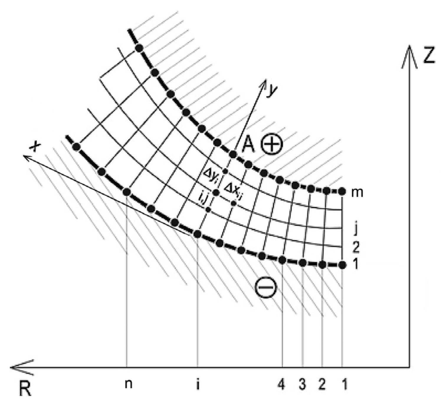
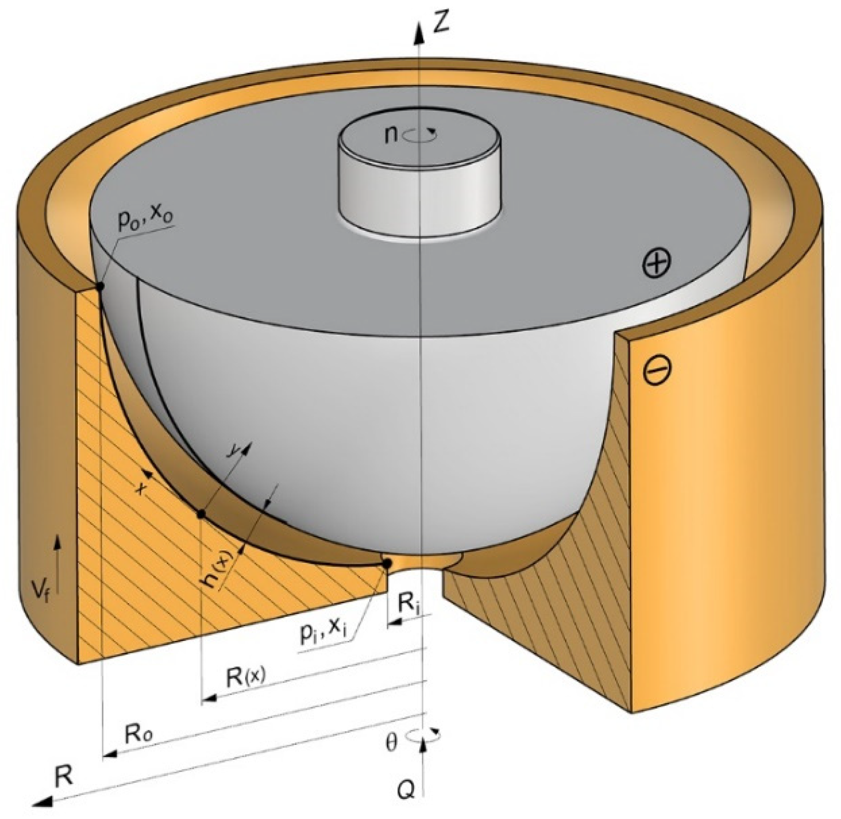
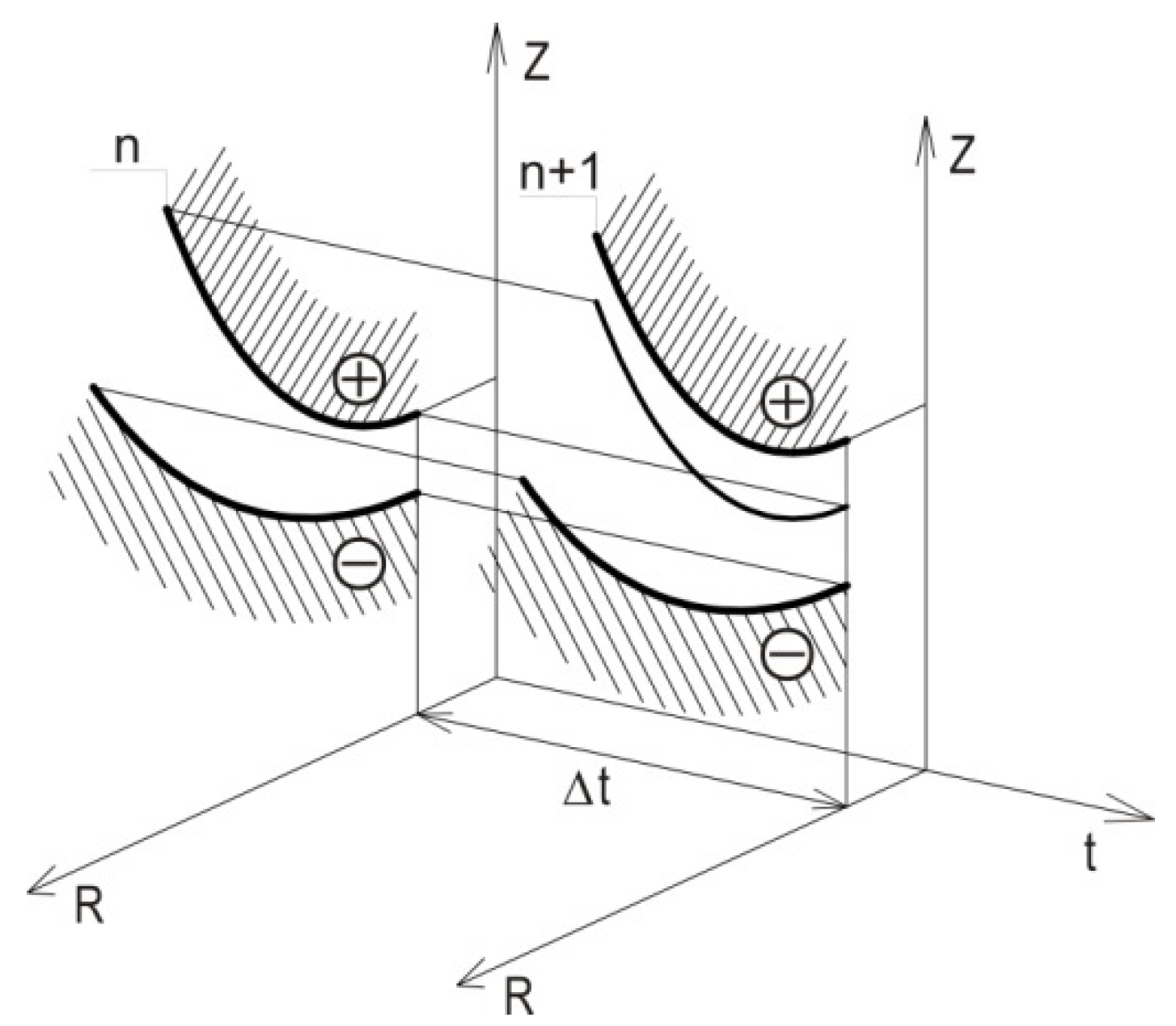
2.2. Theoretical Analysis of ECM Process
- the flow of the mixture (electrolyte, hydrogen) is two-phase, homogeneous, non-slip,
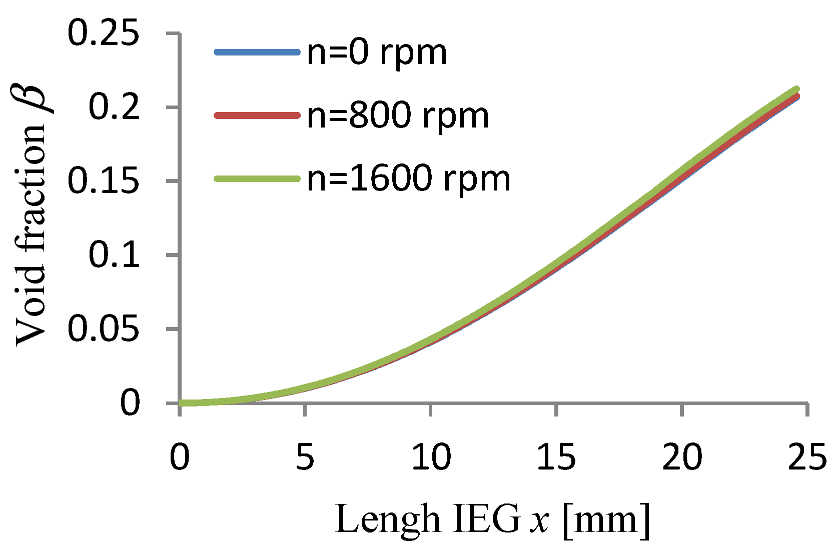
- the distribution of the gas phase results from the intensity of the treatment process and is determined by the volume concentration of hydrogen β(x),
- the phase of the digestion products of the anode is omitted,
- the anode oxygen phase is omitted (the current efficiency of oxygen is assumed to be zero),
- the temperature and pressure of the gas in the bubbles are equal to the temperature and pressure of its surroundings,
- the value of the electrochemical digestion coefficient kV is determined on the basis of experimental tests of the anode-electrolyte-cathode set,
- to determine the hydrodynamic parameters, a stationary (steady), two-dimensional (axisymmetric) flow of the electrolyte and hydrogen mixture is assumed.
- -
- flow continuity equations for electrolyte and hydrogen, respectively:
- -
- momentum equations:
- -
- velocity components:
- -
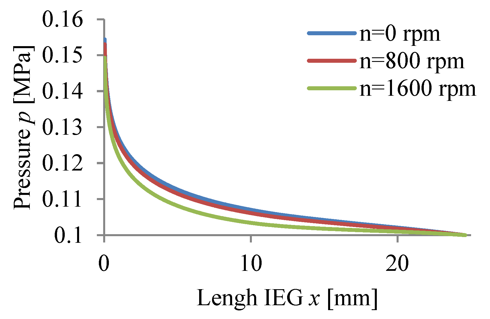
- pressure:
- -
- for temperature:
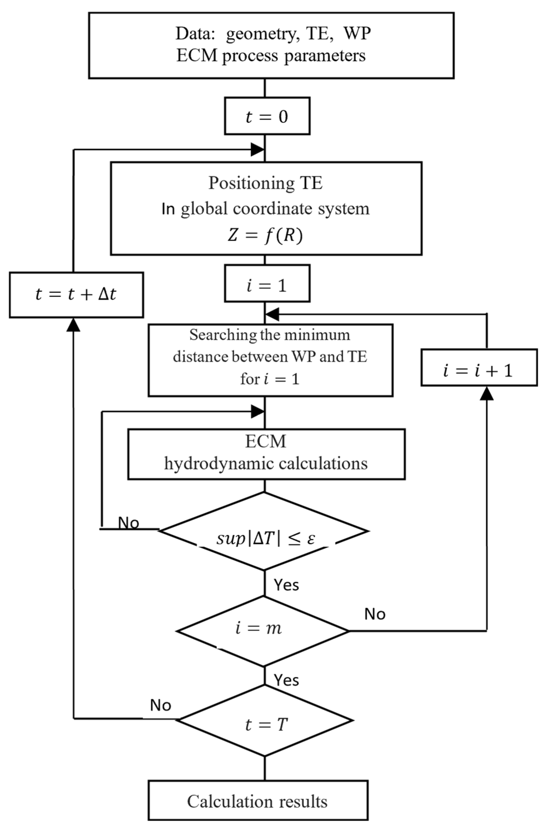
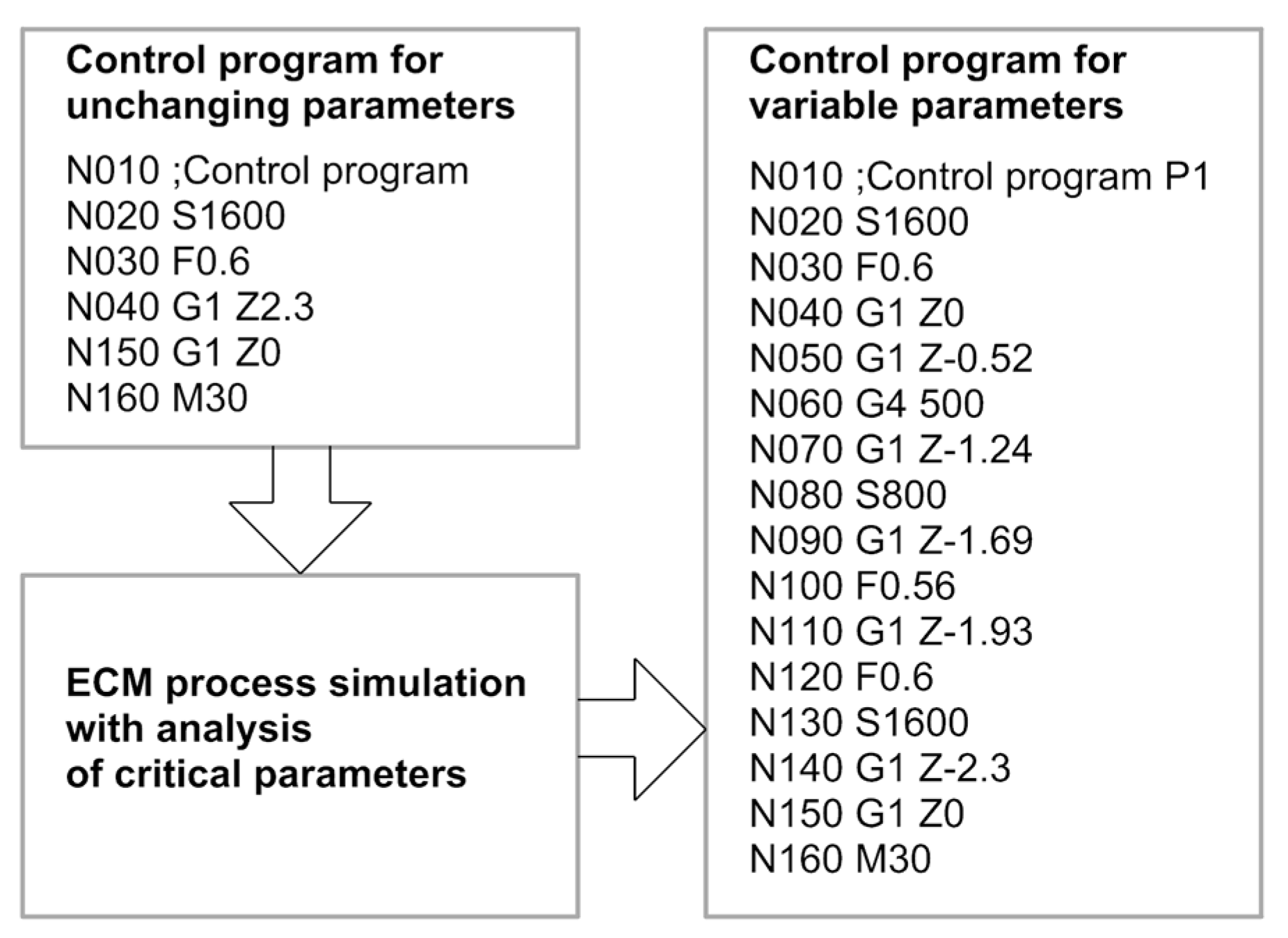
2.3. Computer Simulation of ECM Process
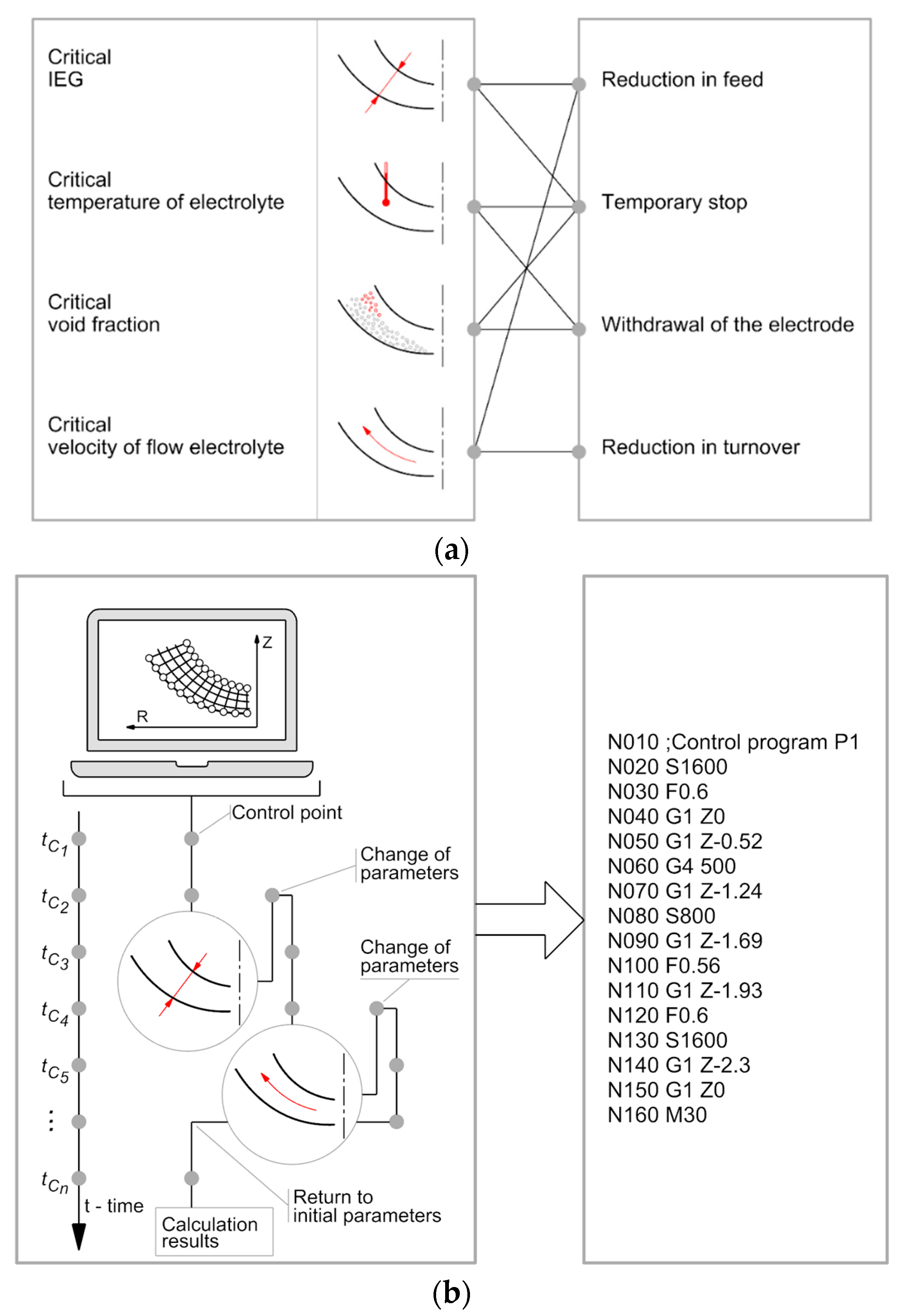
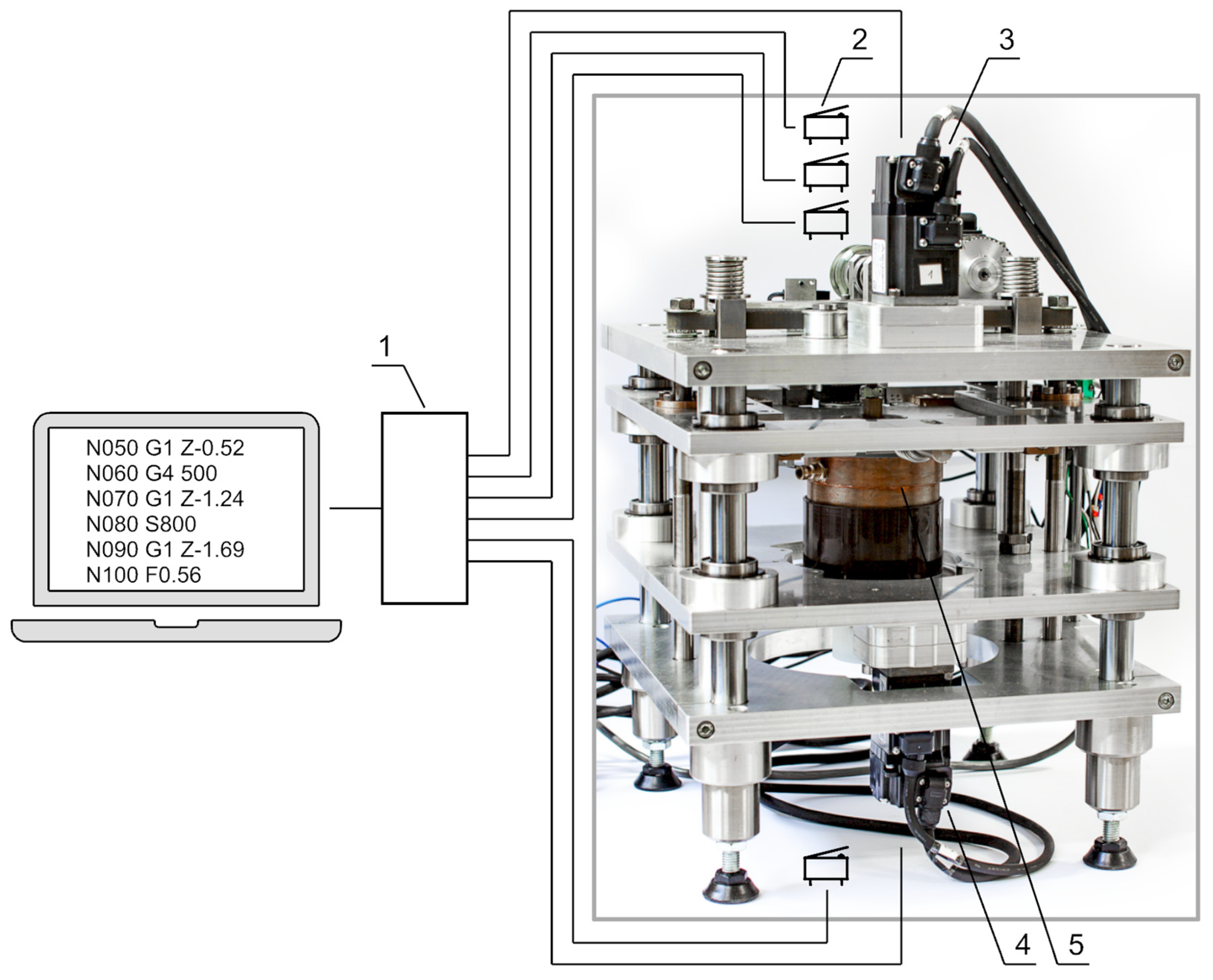
2.4. Adaptive Control
3. Results
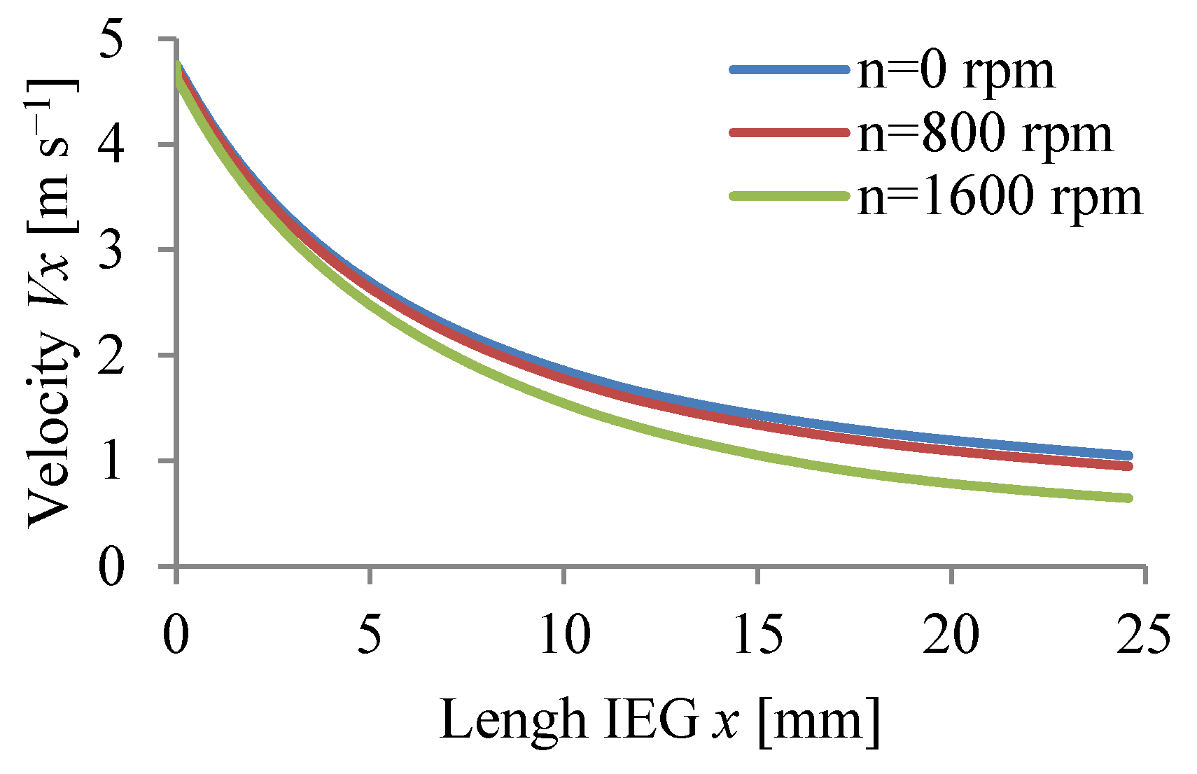
3.1. Results of Simulation of ECM Process
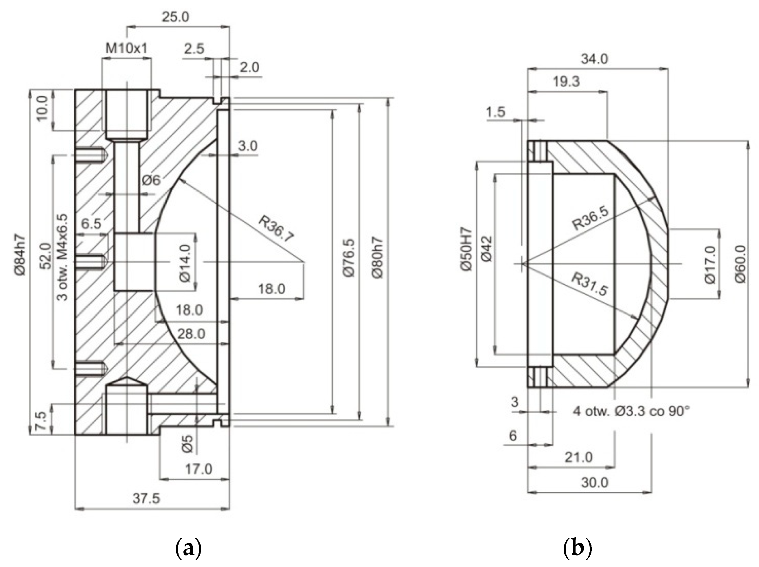
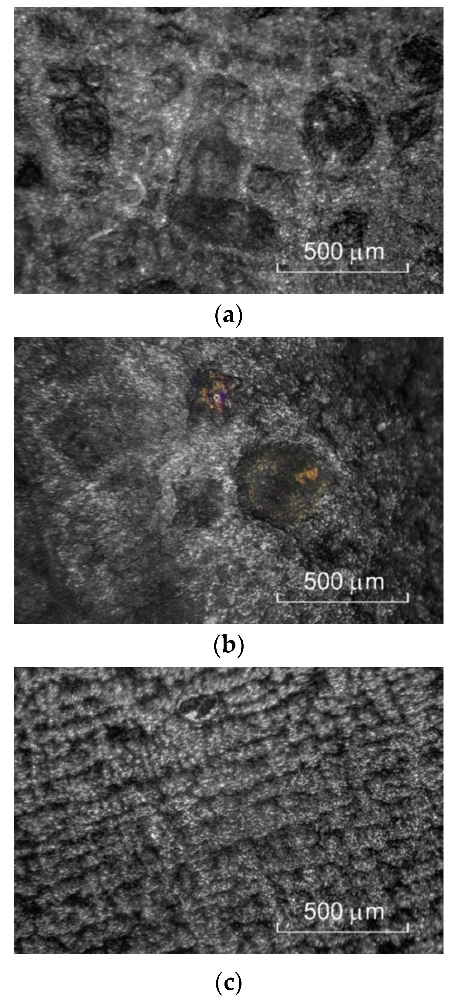
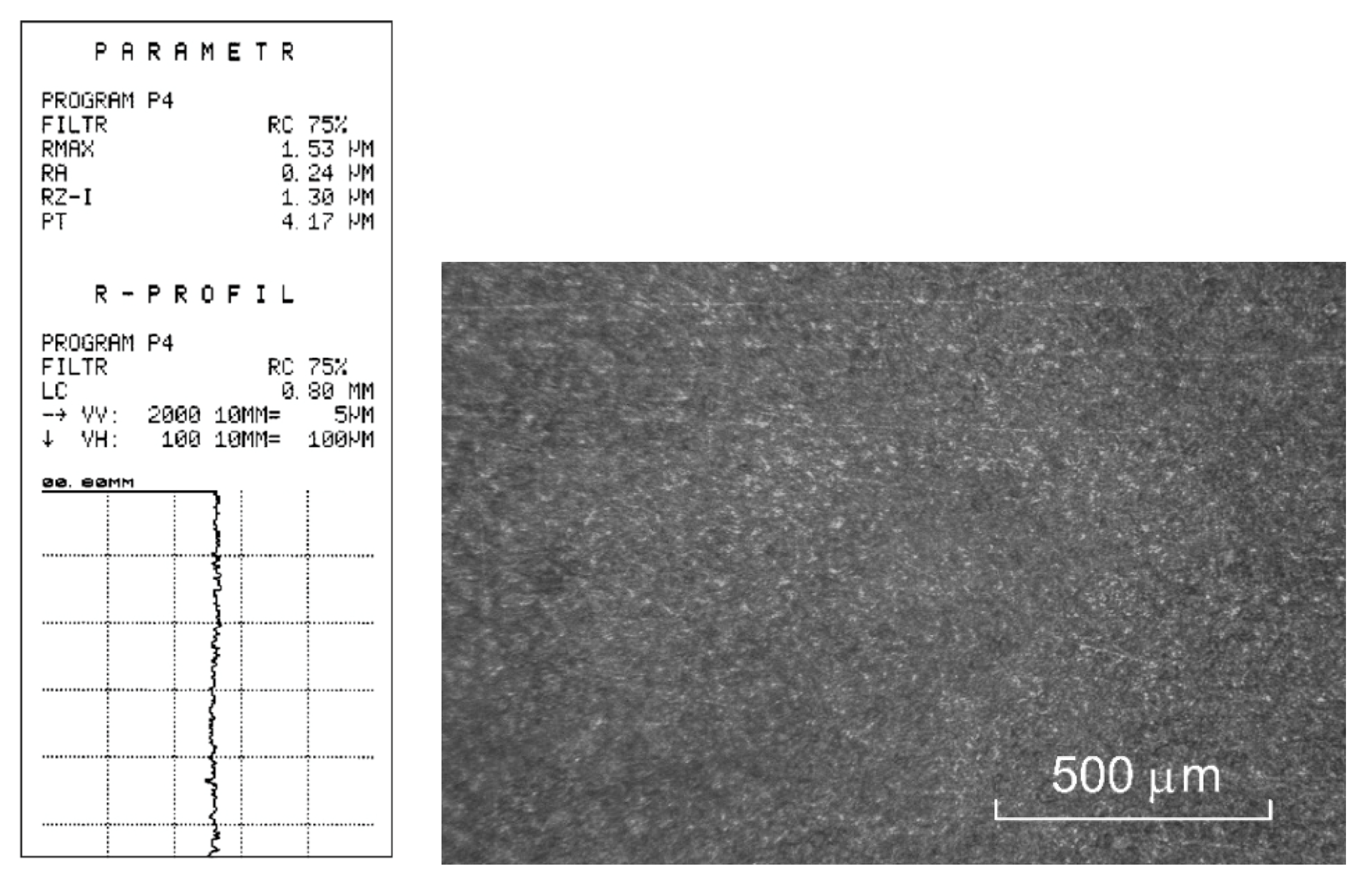
3.2. Experimental Verification
- mathematical model,
- adaptive control.
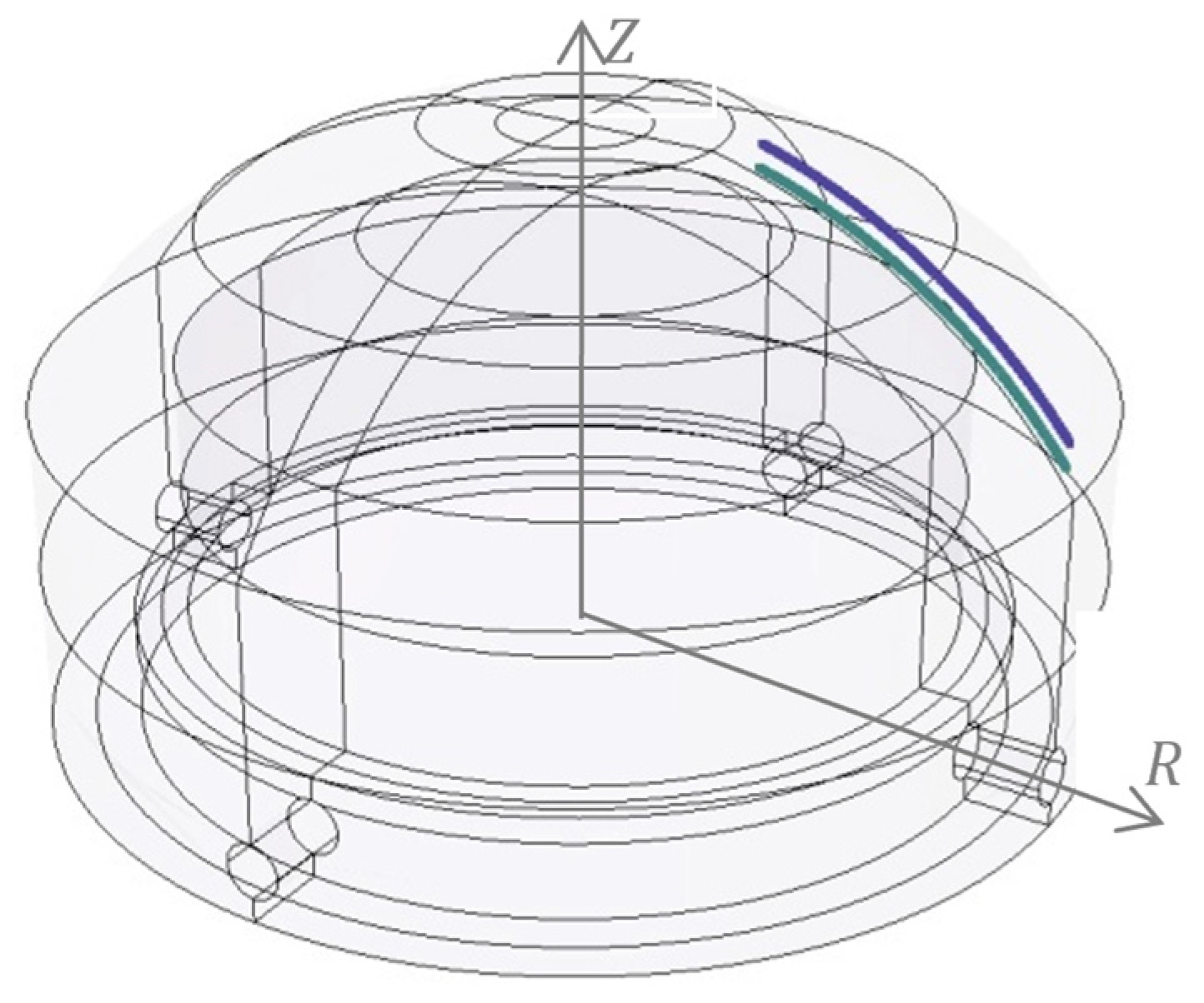
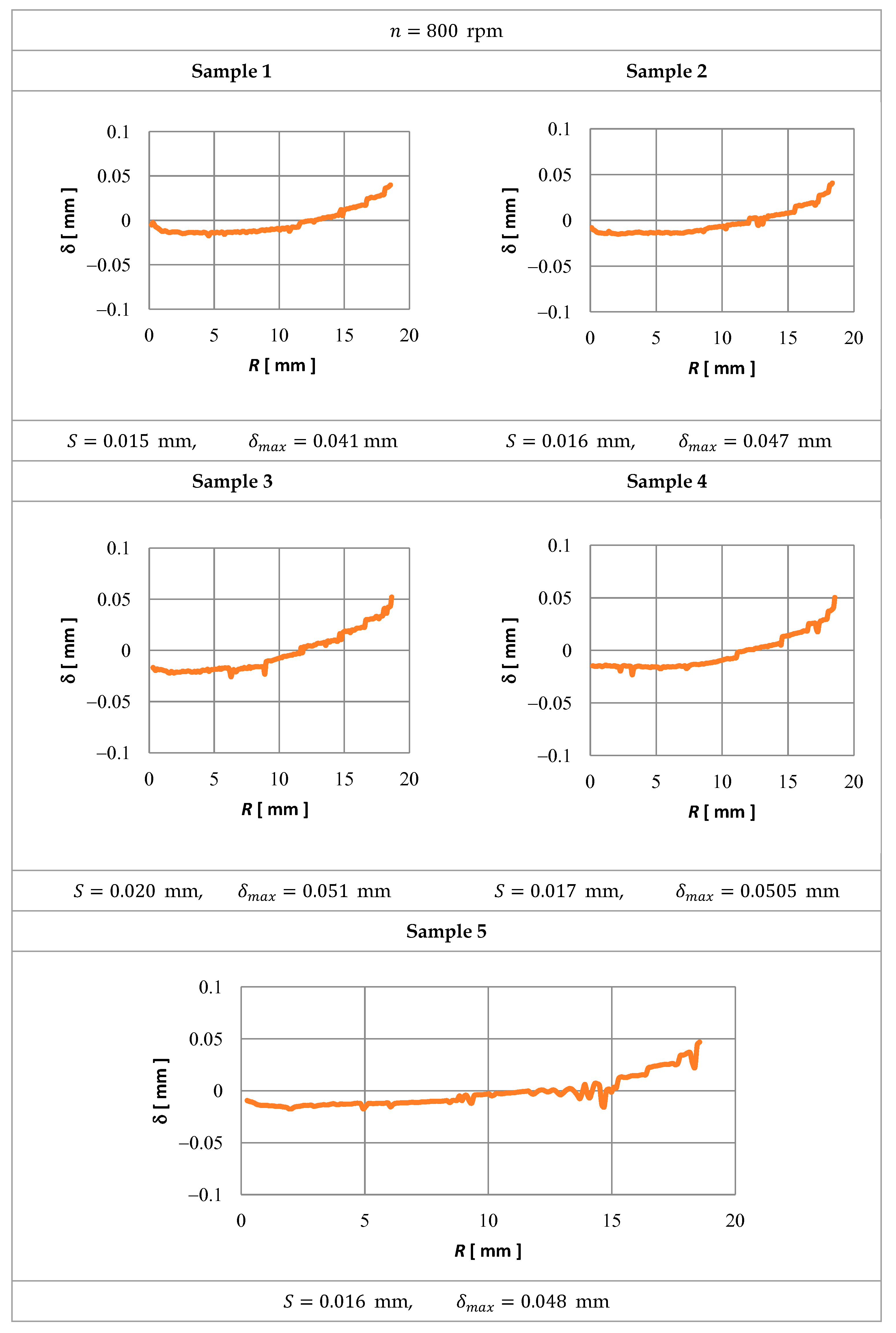
- δ—distribution of the shape deviation (WP) calculated from the process computer simulation (theoretical simulation) and after the ECM,
- δmax—maximum deviation.
4. Discussion
5. Conclusions
Author Contributions
Funding
Institutional Review Board Statement
Informed Consent Statement
Data Availability Statement
Conflicts of Interest
References
- Gusiew, W.N. British Patent 335 003, 1928.
- Gusiew, W.N.; Rożkow, L.A. Autors Certificate 28384. 1928. [Google Scholar]
- Bannard, J. Electrochemical machining—Review. J. Appl. Electrochem. 1977, 7, 1–21. [Google Scholar] [CrossRef]
- Wilson, J.F. Practice and Theory of Electrochemical Machining; Wiley: New York, NY, USA, 1971. [Google Scholar]
- Rajurkar, K.P.; Sundaramb, M.M.; Malshec, M.M. Review of Electrochemical and Electrodischarge Machining. Procedia CIRP 2013, 6, 13–26. [Google Scholar] [CrossRef] [Green Version]
- Rajurkar, K.P.; Zhu, D.; McGeough, J.A.; Kozak, J.; De Silva, A. New developments in electro-chemical machining. Ann. CIRP 1999, 48, 567–579. [Google Scholar] [CrossRef]
- Ruszaj, A.; Gawlik, J.; Skoczypiec, S. Electrochemical machining—Special equipment and applications in aircraft industry. Manag. Prod. Eng. Rev. 2016, 7, 34–41. [Google Scholar] [CrossRef] [Green Version]
- Sawicki, J. Analysis and Modeling of Electrochemical Machining of Curvilinear Rotary Surfaces; Scientific Dissertations No. 164; UTP University of Science and Technology: Bydgoszcz, Poland, 2013. [Google Scholar]
- Dąbrowski, L. Basics of computer simulation of electrochemical forming. In Scientific Works, Mechanics 154; Publisher of Warsaw University of Technology: Warsaw, Poland, 1992. [Google Scholar]
- Kozak, J. Surface shaping contactless electrochemical machining. In Scientific Works, Mechanics 41; Publisher of Warsaw University of Technology: Warsaw, Poland, 1976. [Google Scholar]
- Pott, P.G. Modern electrochemical machining in practice. In Proceedings of the International Symposium for Electro-Machining (ISEM-9), Nagoya, Japan, 9 October 1989; pp. 146–150. [Google Scholar]
- Singh, M.; Singh, S. Electrochemical discharge machining: A review on preceding and perspective research. Proc. Inst. Mech. Eng. Part B J. Eng. Manuf. 2019, 233, 1425–1449. [Google Scholar] [CrossRef]
- Hourng, L.W.; Chang, C.S. Numerical simulation of two-dimensional fluid f1ow in electrochemical drilling. J. Appl. Electrochem. 1994, 24, 1170–1175. [Google Scholar] [CrossRef]
- Kozak, J.; Łubkowski, K.; Dąbrowski, L.; Perończyk, J. Electrochemical Milling. Rzeszów. In Proceedings of the Conference: Manufacture of Machine Components from Alloys with Special Properties; 1985; pp. 172–177. [Google Scholar]
- Kozak, J.; Łubkowski, K.; Dąbrowski, L.; Perończyk, J. Electrochemical milling of shaped surfaces. In Proceedings of the Conference EM’86 (Electromachining), Bydgoszcz, Poland; 1986; pp. 85–91. [Google Scholar]
- Wang, D.Y.; Li, J.Z.; Zhu, D. Counter-rotating electrochemical machining of a convex array using a cylindrical cathode tool with multifold angular velocity. J. Electrochem. Soc. 2019, 166, 412–419. [Google Scholar] [CrossRef]
- Wang, D.Y.; Zhu, Z.W.; Wang, H.R.; Zhu, D. Convex shaping process simulation during counter-rotating electrochemical machining by using the finite element method. Chin. J. Aeronaut. 2016, 29, 534–541. [Google Scholar] [CrossRef] [Green Version]
- He, B.; Wang, D.Y.; Zhu, Z.W.; Li, J.Z.; Zhu, D. Research on counter-rotating electrochemical machining of convex structures with different heights. Int. J. Adv. Manuf. Technol. 2019, 104, 3119–3127. [Google Scholar] [CrossRef]
- Hofstede, A.; van Den Berkel, W.M. Some remarks on electrochemical turning. Annal. CIRP. 1970, 19, 93–106. [Google Scholar]
- Hourng, L.W.; Chang, C.S. Numerical simulation of electrochemical drilling. J. Appl. Electrochem. 1993, 23, 316–321. [Google Scholar] [CrossRef]
- Yun, N.Z. Investigation on application of electrochemical contourevolution machining. In Proceedings of the International Symposium for Electro-Machining (ISEM-9), Nagoya, Japan, 9 October 1989; pp. 143–145. [Google Scholar]
- Tipton, H. The determination of tool shape for ECM. Mach. Prod. Eng. 1968, 2, 325–328. [Google Scholar]
- Akinson, J.; Noble, C. The surface finish resulting from peripherial electrochemical grinding. In Proceedings of the Twenty-Second International Machine Tool Design and Research Conference, Manchester, UK, 16–18 September 1981; pp. 371–378. [Google Scholar] [CrossRef]
- Kubota, M. Mechanical cutting ability of electrochemical grinding wheels. In Proceedings of the 6th Intl Symp Electro-Machining (ISEM-6), Kraków, Poland, 1–5 September 1980; pp. 365–367. [Google Scholar]
- Risko, D. ECM-Current and coming capabilities. In Proceedings of the Nontraditional Machining Symposium, Orlando, FL, USA; 1991. [Google Scholar]
- Ruszaj, A.; Zybura-Skrabalak, M. The mathematical modelling of electrochemical machining with flat ended universal electrodes. J. Mater. Process. Technol. 2001, 109, 333–338. [Google Scholar] [CrossRef]
- Szmaniew, W. Tiechnologia Elektrochimiczeskoj Obrabotki Dietaliej w Awiadwigatieliestrojenii. Izdatielstwo Moskiewskij Uniwersitet; Maszinostrojenie: Moscow, Russia, 1986. [Google Scholar]
- Capello, G. A new approach by electrochemical finishing of hardened cylindrical gear tooth face. CIRP Ann. 1979, 28, 103–107. [Google Scholar]
- Datta, M.; Romankiv, L.T. Application of chemical and electrochemical micromachining in the electronics industry. J. Electrochem. Soc. 1989, 136, 285–292. [Google Scholar] [CrossRef]
- Gieworkian, G.; Szepiel, W. Electrochemical deburring and hole drilling. In Proceedings of the 6th Intl Symp Electro-Machining (ISEM-6), Kraków, Poland, 1–5 September 1980; pp. 349–351. [Google Scholar]
- Gracham, D. Electrochemical deburring. In Proceedings of the 20th MTDR Conference, Birmingham, UK, 12–14 September 1979; pp. 613–616. [Google Scholar]
- Dąbrowski, L.; Łupkowski, K.; Kozak, J.; Rozenek, M. Electrochemical finishing of machine parts. In Proceedings of the 10th international symposium ISEM-X, Magdeburg, Germany, 6–8 May 1992; pp. 529–535. [Google Scholar]
- Dietz, H.; Gonther, K.G.; Otto, K.; Stark, G. Electrochemical turning considerations on machining notes which can be obtained. Ann. CIRP 1979, 28, 93–97. [Google Scholar]
- Barker, A.J. Some aspects of Bosch ECM activities. In Machinery and Production Engineering; Findlay Publications Ltd.: Findlay, OH, USA, 1970; pp. 122–127. [Google Scholar]
- Masuzawa, T.; Sakai, S. Quick Finishing of WEDM Products by ECM Using a Mate-Electrode. CIRP Ann. 1987, 36, 123–126. [Google Scholar] [CrossRef]
- Davydov, A.D.; Volgin, V.M.; Lyubimov, V.V. Electrochemical Machining of Metals: Fundamentals of Electrochemical Shaping. Russ. J. Electrochem. 2004, 40, 1230–1265. [Google Scholar] [CrossRef]
- Kulkarni, A. Electrochemical discharge machining process. Def. Sci. J. 2007, 57, 765–770. Available online: https://core.ac.uk/download/pdf/333720227.pdf (accessed on 28 October 2022). [CrossRef] [Green Version]
- McGeough, J.A. Principles of Electrochemical Machining; Chapman and Hall: London, UK, 1974; 255p. [Google Scholar]
- Mukherjee, S.K.; Kumar, S.; Srivastava, P.K. Effect of electrolyte on the current-carrying process in electrochemical machining. Proc. Inst. Mech. Eng. Part C J. Mech. Eng. Sci. 2007, 221, 1415–1419. [Google Scholar] [CrossRef]
- Alder, G.M.; Clifton, D.; Mill, F. A direct analytical solution to the tool design problem in electrochemical machining under steady state. Proc. Inst. Mech. Eng. 2000, 214, 745–750. [Google Scholar] [CrossRef]
- Cheng, C.P.; Wu, K.L.; Mai, C.C.; Yang, C.K.; Hsu, Y.S.; Yan, B.H. Study of gas film quality in electrochemical discharge machining. Int. J. Mach. Tools Manuf. 2010, 50, 689–697. [Google Scholar] [CrossRef]
- Pattavanitch, J.; Hinduja, S.; Atkinson, J. Modelling of the electrochemical machining process by the boundary element method. CIRP Ann. 2010, 59, 243–246. [Google Scholar] [CrossRef]
- Sawicki, J.; Paczkowski, J. Effect of the hydrodynamic conditions of electrolyte flow on critical states in electrochemical machining. EPJ Web Conf. 2015, 92, 02078. [Google Scholar] [CrossRef] [Green Version]
- Filatov, E.I. The numerical of the unsteady ECM process. J. Mater. Process. Technol. 2001, 109, 327–332. [Google Scholar] [CrossRef]
- Jain, V.K.; Pandey, P.C. Finite element approach to the two-dimensional analysis of electrochemical machining. Proc. Eng. 1980, 2, 23–28. [Google Scholar] [CrossRef]
- Purcar, M.; Bortels, L.; Van den Bossche, B.; Deconinck, J. 3D electrochemical machining computer simulations. J. Mater. Process. Technol. 2004, 149, 472–478. [Google Scholar] [CrossRef]
- Purcar, M.; Dorochenko, A.; Bortels, L.; Deconinck, J.; Van den Bossche, B. Advanced CAD integrated approach for 3D electrochemical machining simulations. J. Mater. Process. Technol. 2008, 203, 58–71. [Google Scholar] [CrossRef]
- Chang, C.S.; Hourng, L.W. Two-dimensional two-phase numerical model for tool design in electrochemical machining. J. Appl. Electrochem. 2001, 31, 145–154. [Google Scholar] [CrossRef]
- Chang, C.S.; Hourng, L.W.; Chung, C.T. Tool design in electrochemical machining considering the effect of thermal-fluid properties. J. Appl. Electrochem. 1999, 29, 321–330. [Google Scholar] [CrossRef]
- Vołgin, V.M.; Lyubimov, V.V. Numerical simulation of the electrolyte flow at three-dimensional electrochemical machining. In Proceedings of the APE’2001, Warsaw, Poland, 7–9 June 2001; pp. 299–308. [Google Scholar]
- Dąbrowski, L.; Kozak, J. Electrochemical Machining of Complex Shape Parts and Holes (Mathematical Modeling and Experiments). In Proceedings of the Twenty-Second International Machine Tool Design and Research Conference, Manchester, UK, 16–18 September 1981; pp. 385–392. [Google Scholar]
- Dąbrowski, L.; Paczkowski, T. Computer Simulation of Two-dimensional Electrolyte F1ow in Electrochemical Machining. Russ. J. Electrochem. 2005, 41, 91–98. [Google Scholar] [CrossRef]
- Deconinck, D.; Van Damme, S.; Albu, C.; Hotoiu, L.; Deconinck, J. Study of the effects of heat removal on the copying accuracy of the electrochemical machining process. Electrochim. Acta 2011, 56, 5642–5649. [Google Scholar] [CrossRef]
- Larsson, C.N. Adaptive control of ECM based on flow measurement. In Proceedings of the 6th Intl Symp Electro-Machining (ISEM-6), Kraków, Poland, 1–5 September 1980; pp. 298–300. [Google Scholar]
- Fang, X.; Qu, N.; Zhang, Y.; Xu, Z.; Zhu, D. Effects of pulsating electrolyte flow in electrochemical machining. J. Mater. Process. Technol. 2014, 214, 36–43. [Google Scholar] [CrossRef]
- Kotlyar, L.M.; Minazetdinov, N.M. Modeling of electrochemical machining with the use of a curvilinear electrode and a stepwise dependence of the current efficiency on the current density. J. Appl. Mech. Tech. Phys. 2016, 57, 127–135. [Google Scholar] [CrossRef]
- Thorpe, J.F.; Zerkle, R.D. Analytical Determination of the Equilibrium Electrode Gap in Electrochemical Machining. Int. J. Mach. Tool Des. Res. 1969, 9, 131–144. [Google Scholar] [CrossRef]
- Chai, M.; Li, Z.; Song, X.; Ren, J.; Cui, Q. Optimization and Simulation of Electrochemical Machining of Cooling Holes on High Temperature Nickel-Based Alloy. Int. J. Electrochem. Sci. 2021, 16, 1–15. [Google Scholar] [CrossRef]
- Drake, T.H.; McGeough, J.A. Aspect of drilling by electrochemical ARC machining. In Proceedings of the Twenty-Second International Machine Tool Design and Research Conference, Manchester, UK, 16–18 September 1981; pp. 361–369. [Google Scholar] [CrossRef]
- El-Hofy, H.; McGeough, J.A. Evoluation of an apparatus for electrochemical arc wire machining. Trans. ASME Ser. B 1988, 110, 119–123. [Google Scholar] [CrossRef]
- Zhang, C.; Xu, Z.; Hang, Y.; Xing, J. Effect of solution conductivity on tool electrode wear in electrochemical discharge drilling of nickel-based alloy. Int. J. Adv. Manuf. Technol. 2019, 103, 743–756. [Google Scholar] [CrossRef]
- Kozak, J. Mathematical Models for Computer Simulation of Electrochemical Machining Process. J. Mater. Process. Technol. 1998, 76, 170–175. [Google Scholar] [CrossRef]
- Łubkowski, K. Critical states in electrochemical machining. In Scientific Works, Mechanics 163; Publisher of Warsaw University of Technology: Warsaw, Poland, 1996. [Google Scholar]
- Paczkowski, T.; Sawicki, J. Electrochemical Machining of Curvilinear Surfaces. J. LMST Mach. Sci. Technol. 2008, 12, 33–52. [Google Scholar] [CrossRef]
- Kozak, J.; Dąbrowski, L. Computer aided system for ECM. Surf. Eng. Appl. Electrochem. 1992, 6, 243–255. [Google Scholar]
- Paczkowski, T.; Zdrojewski, J. The mechanism of ECM technology design for curvilinear surfaces. Procedia CIRP 2016, 42, 356–361. [Google Scholar] [CrossRef]
- Hasan, D.; Oguzhan, Y.; Bahattin, K. Controlling short circuiting, oxide layer and cavitation problems in electrochemical. J. Mater. Process. Technol. 2018, 262, 585–596. [Google Scholar]
- Paczkowski, T.; Zdrojewski, J. Monitoring and control of the electrochemical machining process under the conditions of a vibrating tool electrode. J. Mater. Process. Technol. 2017, 244, 204–214. [Google Scholar] [CrossRef]
- Landau, I.D.; Lozano, R.; M’saad, M.; Karimi, A. Adaptive Control, Communications and Control Engineering; Springer-Verlag London Limited: London, UK, 2011. [Google Scholar] [CrossRef]


| Parameters | Specifications |
|---|---|
| Critical IEG | 0.05 mm |
| Critical temperature of electrolyte | 368 K |
| Critical void fraction | 0.45 |
| Critical velocity of flow electrolyte | 5 ms−1 |
| Parameters | Specifications | |
|---|---|---|
| Initial gap | 0.2 mm | |
| Feed rate of the TE | 1 mm min−1 | |
| Working voltage | 15 V | |
| Volumetric flow rate | 3 dm3 min−1 | |
| Outlet pressure | 0.1 MPa | |
| Machining time | 60 s | |
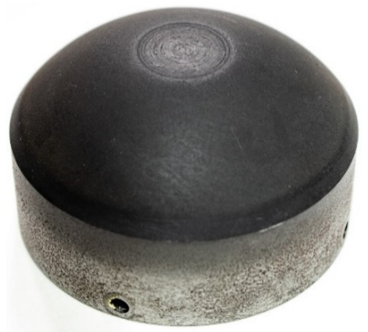
| Workpiece material | WP | alloy tool steel 2312 |
| Electrochemical machinability: | =1.59 (1 − exp(2.56 − 0.112j) mm3 (A min)−1, j A cm−2 | |
| electrolyte | 15% water solution of NaNO3 |
| Sample No. | δ [mm] | S [mm] |
|---|---|---|
| Sample 1 | 0.33 | 0.012 |
| Sample 2 | 0.34 | 0.013 |
| Sample 3 | 0.33 | 0.012 |
Publisher’s Note: MDPI stays neutral with regard to jurisdictional claims in published maps and institutional affiliations. |
© 2022 by the authors. Licensee MDPI, Basel, Switzerland. This article is an open access article distributed under the terms and conditions of the Creative Commons Attribution (CC BY) license (https://creativecommons.org/licenses/by/4.0/).
Share and Cite
Sawicki, J.; Paczkowski, T. Electrochemical Machining of Curvilinear Surfaces of Revolution: Analysis, Modelling, and Process Control. Materials 2022, 15, 7751. https://doi.org/10.3390/ma15217751
Sawicki J, Paczkowski T. Electrochemical Machining of Curvilinear Surfaces of Revolution: Analysis, Modelling, and Process Control. Materials. 2022; 15(21):7751. https://doi.org/10.3390/ma15217751
Chicago/Turabian StyleSawicki, Jerzy, and Tomasz Paczkowski. 2022. "Electrochemical Machining of Curvilinear Surfaces of Revolution: Analysis, Modelling, and Process Control" Materials 15, no. 21: 7751. https://doi.org/10.3390/ma15217751
APA StyleSawicki, J., & Paczkowski, T. (2022). Electrochemical Machining of Curvilinear Surfaces of Revolution: Analysis, Modelling, and Process Control. Materials, 15(21), 7751. https://doi.org/10.3390/ma15217751