
Corrosion Behavior and Mechanical Properties of 30CrMnSiA High-Strength Steel under an Indoor Accelerated Harsh Marine Atmospheric Environment


Abstract
:1. Introduction
2. Experimental Procedures
2.1. Materials and Alternate Immersion Test
2.2. Corrosion Kinetic Analysis
2.3. Surface Morphology Observation and Composition Identification
2.4. Electrochemical Measurement
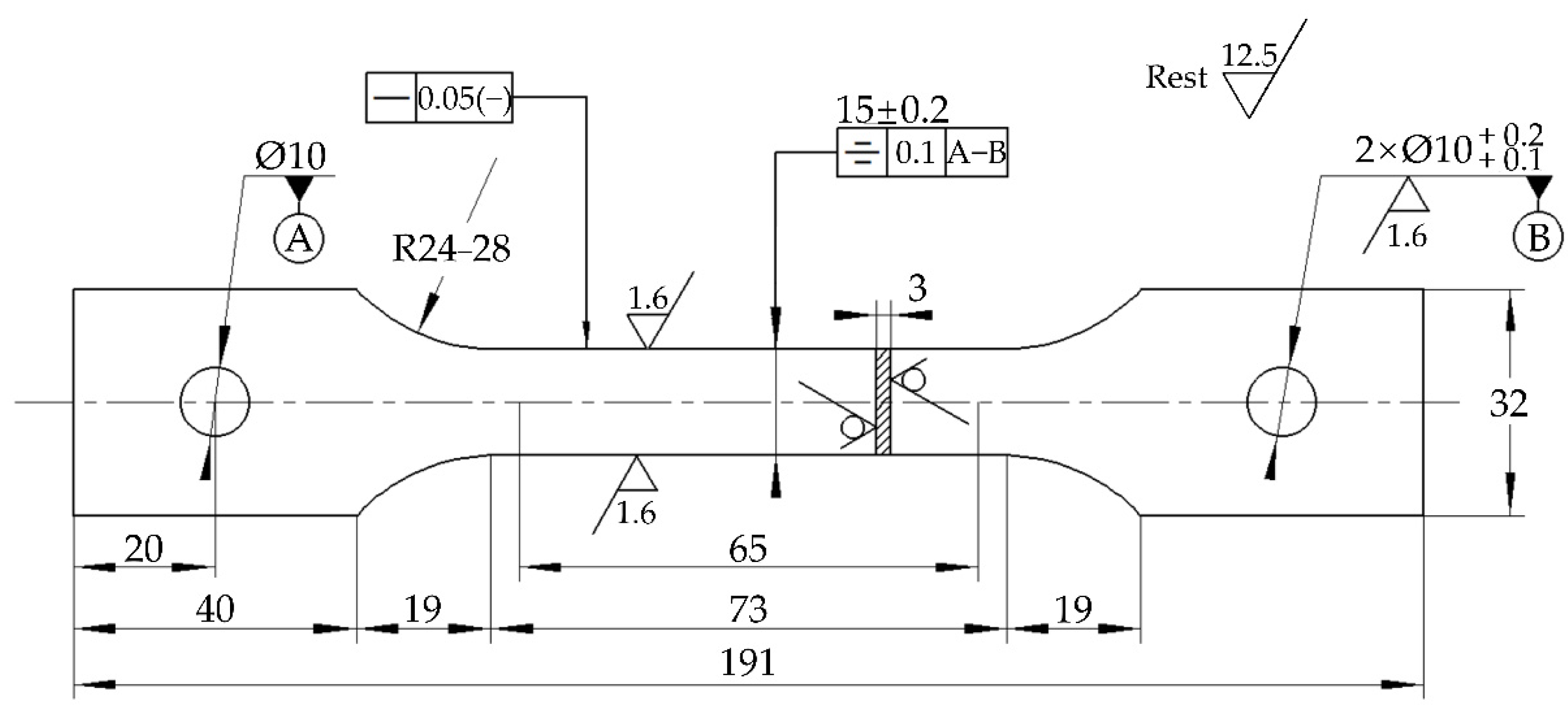
2.5. Mechanical Property Test
3. Results and Discussion
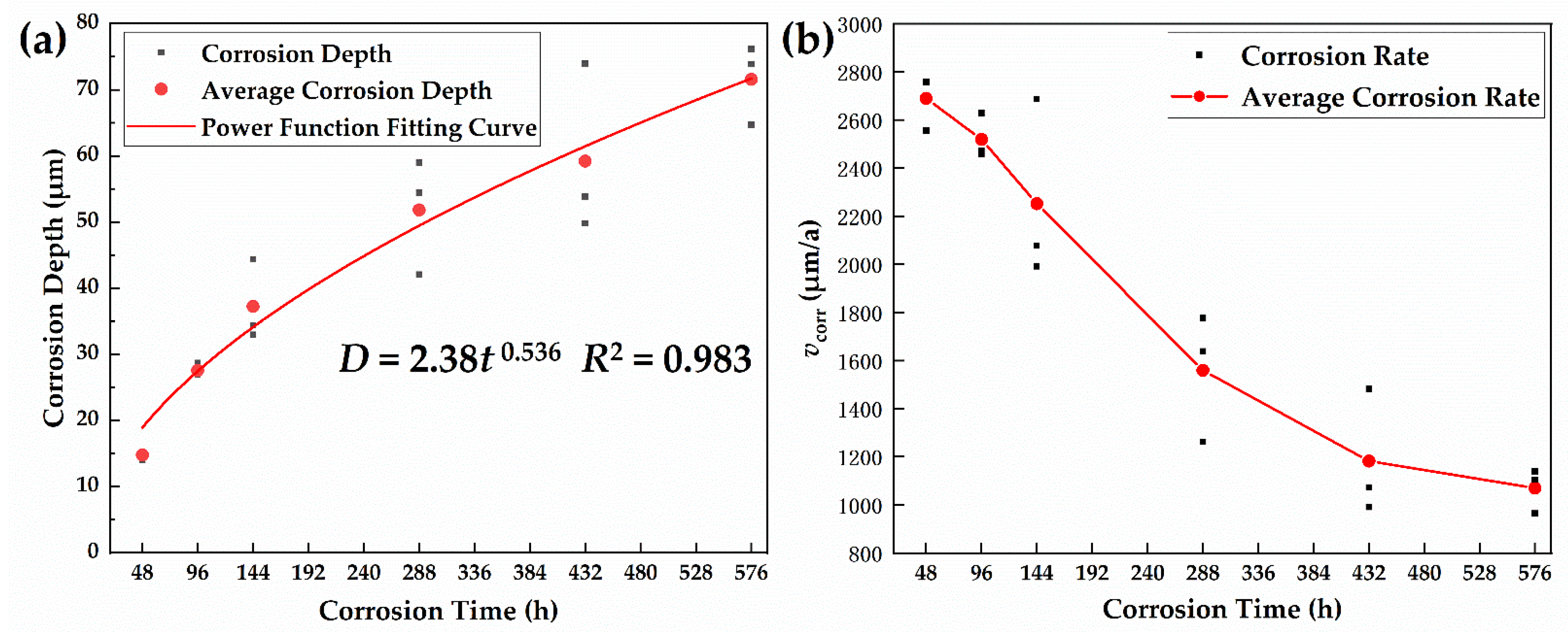
3.1. Corrosion Kinetic Analysis
3.2. Surface Microstructure Analysis
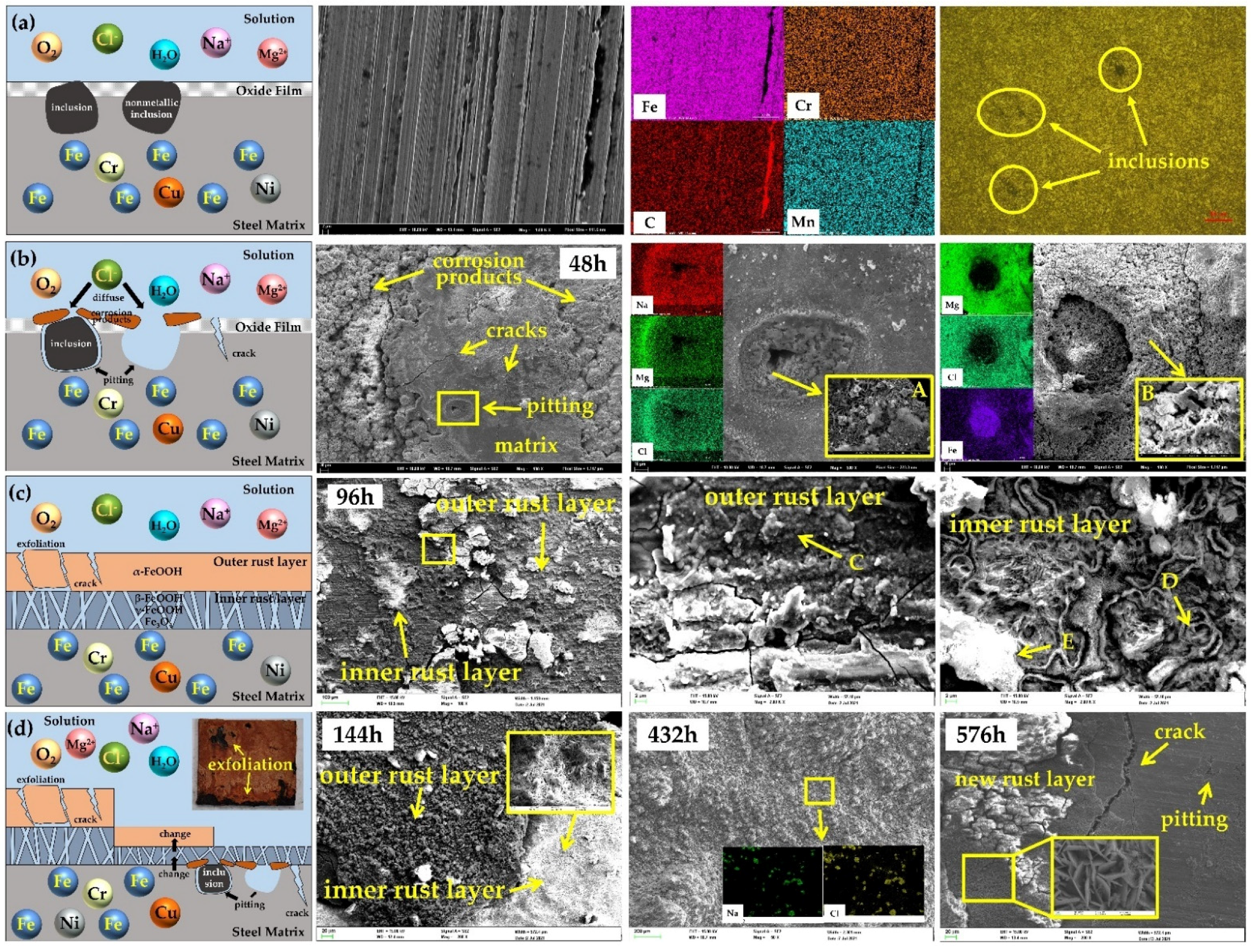
3.2.1. Surface Morphologies of Corrosion Products
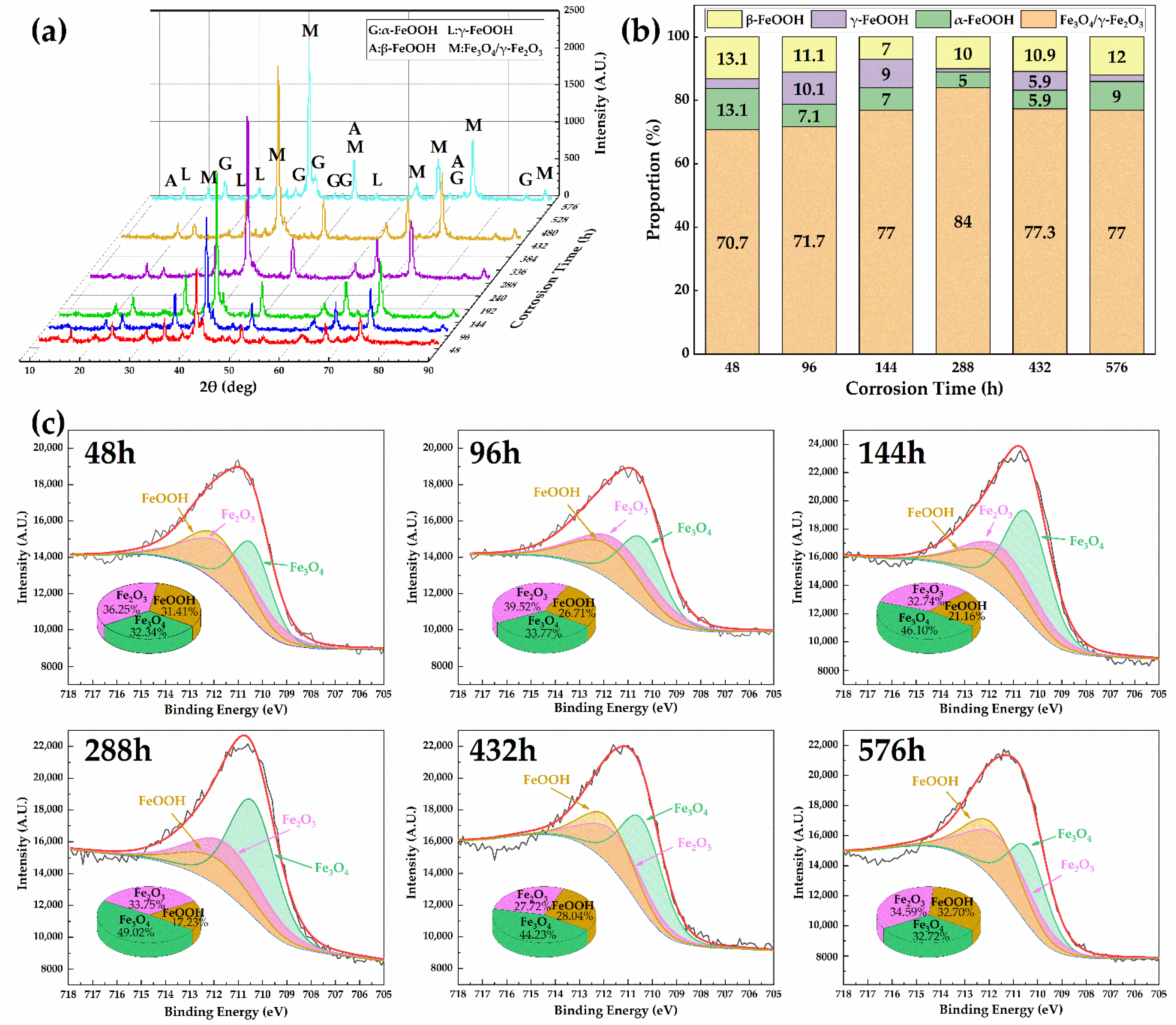
3.2.2. Composition of the Rust Layer
3.3. Electrochemical Tests
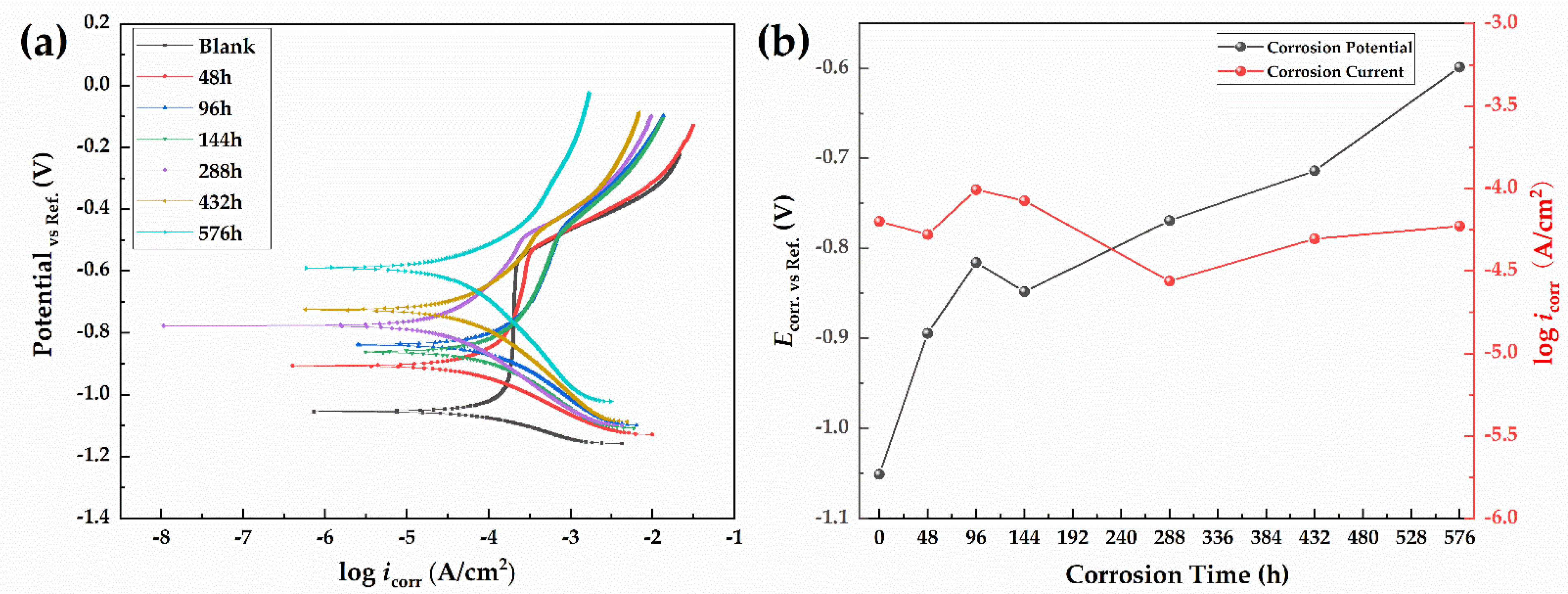
3.3.1. Potentiodynamic Polarization Curves
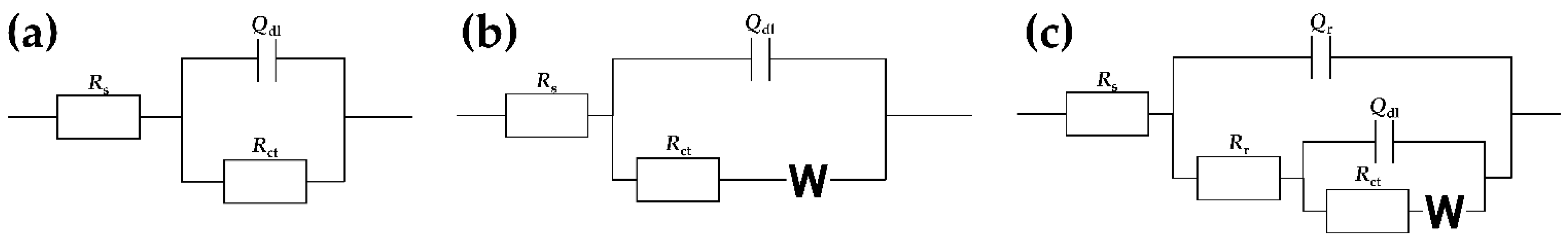
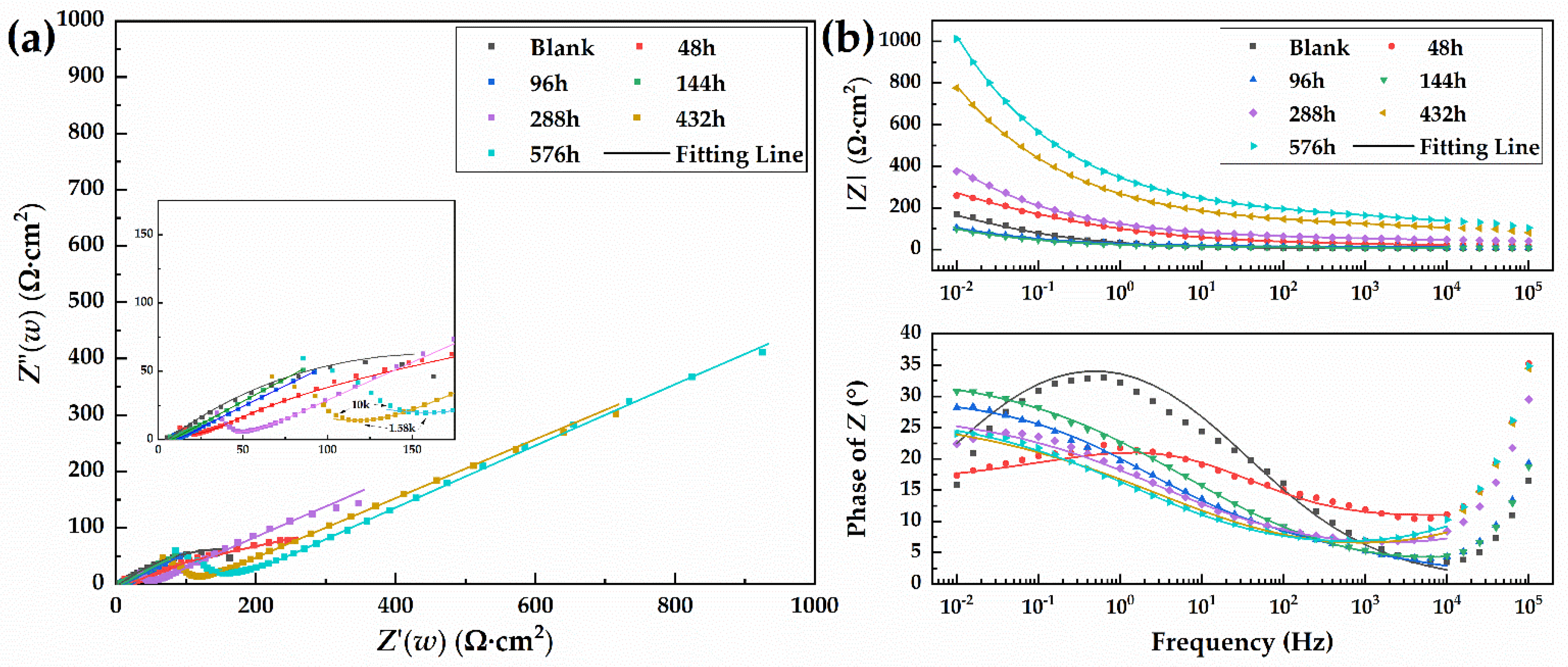
3.3.2. Electrochemical Impedance Spectroscopy (EIS)
3.4. Mechanical Property Test
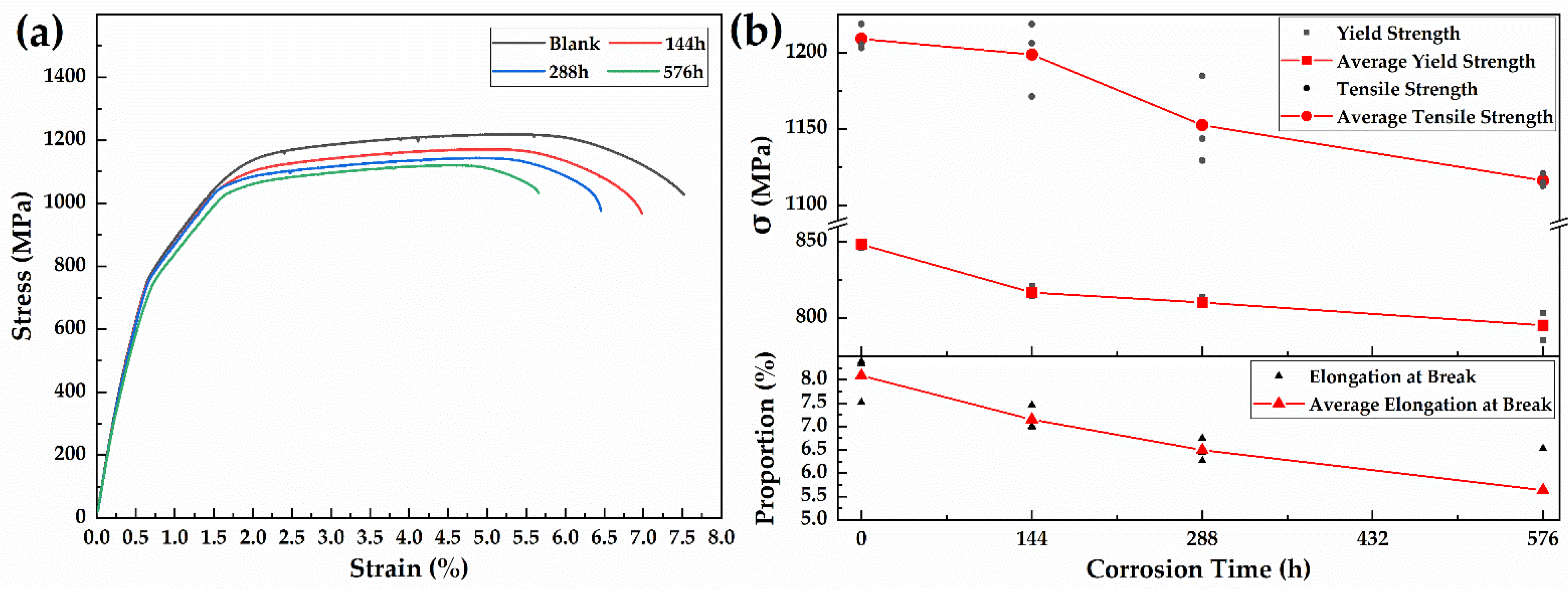
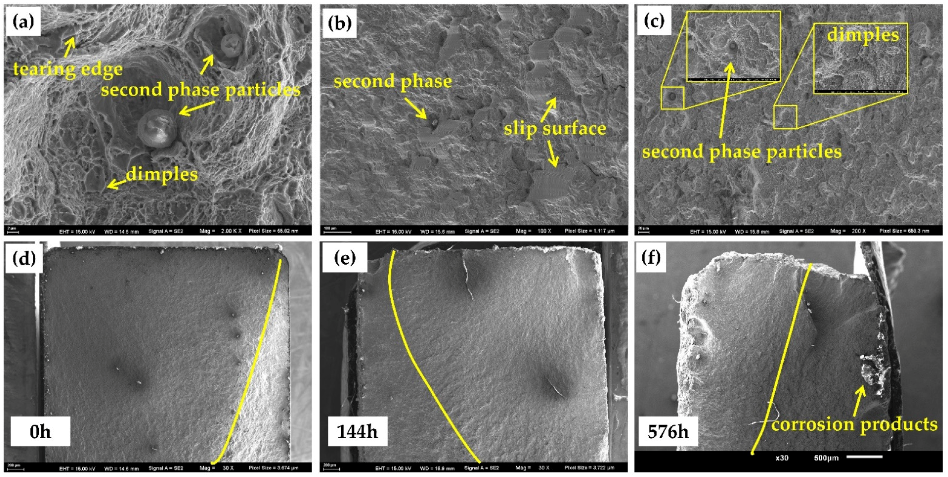
3.4.1. Tensile Test
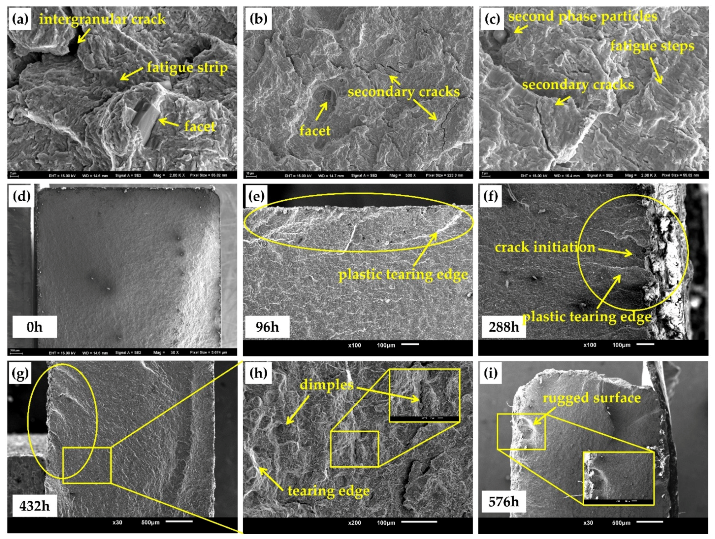
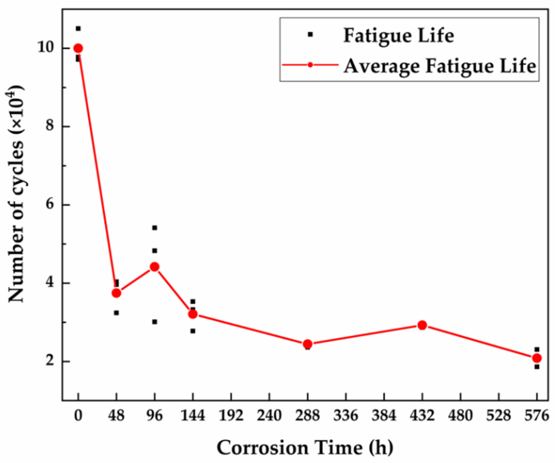
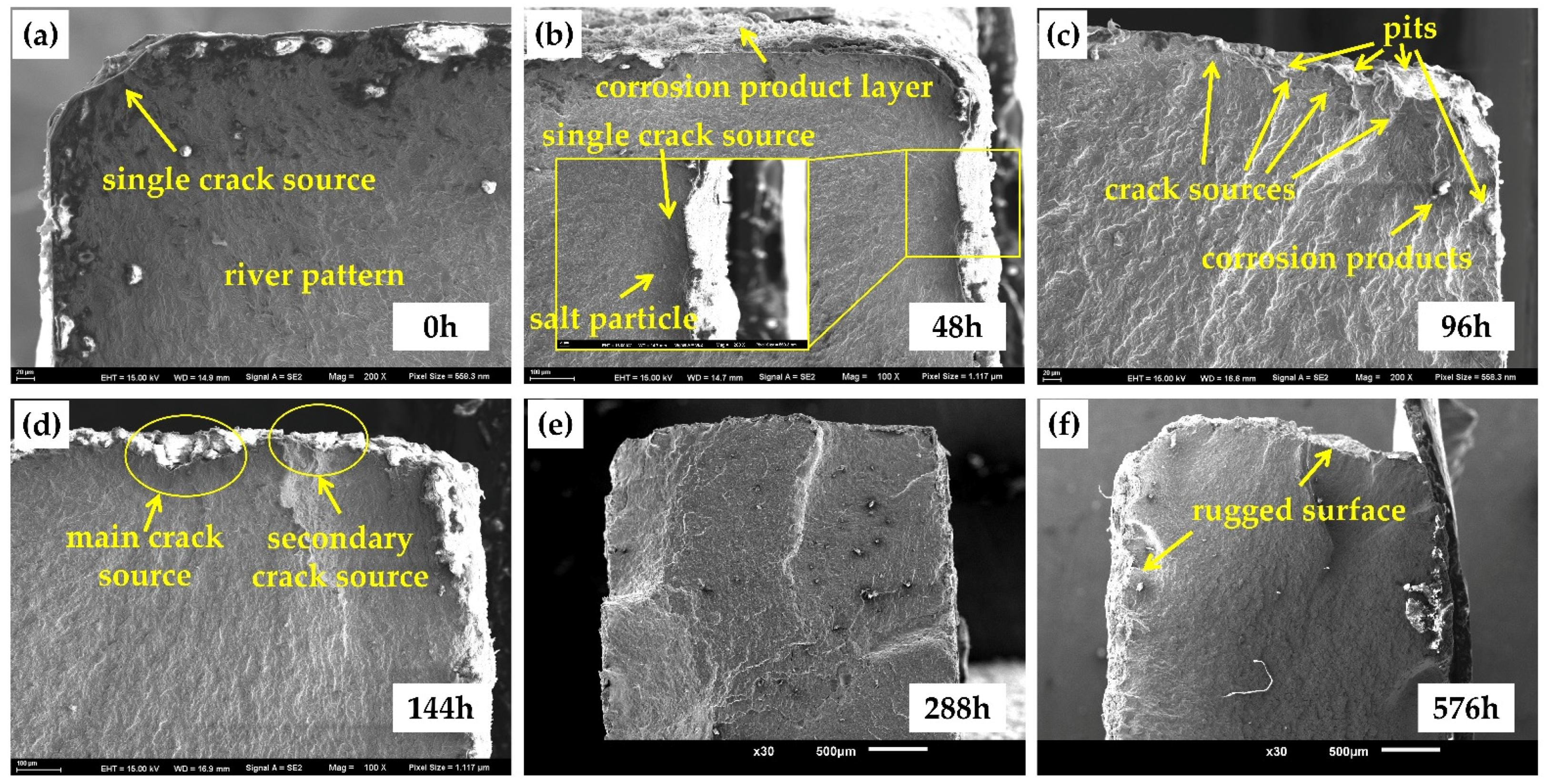
3.4.2. Fatigue Test
4. Conclusions
- The corrosion kinetics of the 30CrMnSiA high-strength steel followed the power function after 576 h of corrosion, which proves that the material has good corrosion resistance. The test scheme also showed good acceleration.
- The rust layer contains abundant goethite, magnetite, and maghemite, which have dense structures and can effectively protect the matrix from corrosive solutions.
- The atmospheric corrosion of 30CrMnSiA high-strength steel starts from a pitting corrosion and gradually leads to exfoliation. The corrosion enters a cycle. Firstly, the surface of the matrix gradually becomes the inner rust layer due to the occurrence of corrosion, and the inner rust layer then grows and becomes the outer rust layer. Finally, the outer rust layer falls off, exposing the inner rust layer to the corrosive environment and providing a channel for the corrosive medium to attack the matrix.
- Electrochemical tests further prove that the protective effect of the rust layer on the matrix becomes stronger with the development of corrosion and tends to be stable.
- The tensile and fatigue properties of 30CrMnSiA decreases after corrosion. After 576 h of corrosion, the tensile strength, yield strength, and elongation at break decreased by 6.25%, 7.69%, and 30.27%, respectively. The influence of corrosion on fatigue performance was evaluated from three stages of fatigue fracture. In the crack initiation stage, which occupies most of the fatigue life of specimens, due to the pitting that occurred, the fatigue life reduced by 50%.
Author Contributions
Funding
Institutional Review Board Statement
Informed Consent Statement
Data Availability Statement
Conflicts of Interest
References
- Cai, Y.K.; Xu, Y.M.; Zhao, Y.; Ma, X.B. Atmospheric corrosion prediction: A review. Corros. Rev. 2020, 38, 299–321. [Google Scholar] [CrossRef]
- Hai, C.; Wang, Z.; Lu, F.Y.; Zhang, S.P.; Du, C.W.; Cheng, X.Q.; Li, X.G. Analysis of Corrosion Evolution in Carbon Steel in the Subtropical Atmospheric Environment of Sichuan. J. Mater. Eng. Perform. 2021, 30, 8014–8022. [Google Scholar] [CrossRef]
- Robrge, P.R.; Klassen, R.D.; Haberecht, P.W. Atmospheric corrosivity modeling—A review. Mater. Design. 2002, 23, 321–330. [Google Scholar] [CrossRef]
- Morcillo, M.; Chico, B.; Diaz, I.; Cano, H.; Fuente, D. Atmospheric corrosion data of weathering steels. A review. Corros. Sci. 2013, 77, 6–24. [Google Scholar] [CrossRef] [Green Version]
- Thierry, D.; Persson, D.; Luckeneder, G.; Stellnberger, K.H. Atmospheric corrosion of ZnAlMg coated steel during long term atmospheric weathering at different worldwide exposure sites. Corros. Sci. 2019, 148, 338–354. [Google Scholar] [CrossRef]
- Jenifer, A.; Fuente, D.; Chico, B.; Simancas, J.; Diaz, I.; Morcillo, M. Marine atmospheric corrosion of carbon steel: A review. Materials 2017, 10, 406. [Google Scholar]
- Melchers, R.E. Long-term corrosion of cast irons and steel in marine and atmospheric environments. Corros. Sci. 2013, 68, 186–194. [Google Scholar] [CrossRef]
- Wu, W.; Dai, Z.Y.; Liu, Z.Y.; Liu, C.; Li, X.G. Synergy of cu and sb to enhance the resistance of 3%ni weathering steel to marine atmospheric corrosion. Corros. Sci. 2021, 183, 109353. [Google Scholar] [CrossRef]
- Xu, X.X.; Cheng, H.L.; Wu, W.; Liu, Z.Y.; Li, X.G. Stress corrosion cracking behavior and mechanism of Fe-Mn-Al-C-Ni high specific strength steel in the marine atmospheric environment. Corros. Sci. 2021, 191, 109760. [Google Scholar] [CrossRef]
- Okayasu, M.; Sato, K.; Okada, K.; Yoshifuji, S.; Mizuno, M. Effects of atmospheric corrosion on fatigue properties of a medium carbon steel. J. Mater. Sci. 2009, 44, 306–315. [Google Scholar] [CrossRef]
- Nekouei, R.K.; Akhaghi, R.; Ravanbakhsh, A.; Tahmasebi, R.; Moghaddam, A.J.; Mahrouei, M. A study of the effect of two-stage tempering on mechanical properties of steel 30CrMnSi using analysis on response surface in design of experiment. Met. Sci. Heat. Treat. 2016, 57, 694–701. [Google Scholar] [CrossRef]
- Yang, X.K.; Zhang, L.W.; Liu, M.; Zhang, S.Y.; Zhou, K.; She, Z.X.; Mu, X.L.; Li, D.F. Atmospheric corrosion behaviour of 30crmnsia high-strength steel in rural, industrial and marine atmosphere environments. Brit. Corros. J. 2017, 52, 226–235. [Google Scholar] [CrossRef]
- Hoerle, S.; Mazaudier, F.; Dillmann, P.; Santarini, G. Advances in understanding atmospheric corrosion of iron. II. Mechanistic modelling of wet–dry cycles. Corros. Sci. 2004, 46, 1431–1465. [Google Scholar] [CrossRef]
- Guo, M.X.; Tang, J.R.; Peng, C.; Li, X.H.; Wang, C.; Pan, C.; Wang, Z.Y. Effects of salts and its mixing ratio on the corrosion behavior of 316 stainless steel exposed to a simulated salt-lake atmospheric environment. Mater. Chem. Phys. 2021, 276, 125380. [Google Scholar] [CrossRef]
- Wu, W.; Cheng, X.Q.; Hou, H.X.; Bo, L.; Li, X.G. Insight into the product film formed on ni-advanced weathering steel in a tropical marine atmosphere. Appl. Surf. Sci. 2018, 436, 80–89. [Google Scholar] [CrossRef]
- Surnam, B.; Chui, C.W.; Xiao, H.P.; Liang, H. Investigating atmospheric corrosion behavior of carbon steel in coastal regions of Mauritius using Raman Spectroscopy. Matéria 2016, 21, 157–168. [Google Scholar] [CrossRef] [Green Version]
- Dong, J.H.; Han, E.H.; Ke, W. Introduction to atmospheric corrosion research in China. Sci. Technol. Adv. Mater. 2007, 8, 559–565. [Google Scholar] [CrossRef] [Green Version]
- Lin, C.C.; Wang, C.X. Correlation between accelerated corrosion tests and atmospheric corrosion tests on steel. J. Appl. Electrochem. 2005, 35, 837–843. [Google Scholar] [CrossRef]
- Calero, J.; Alcantara, J.; Chico, B.; Diaz, I.; Simancas, J.; Fuente, D.; Morcillo, M. Wet/dry accelerated laboratory test to simulate the formation of multilayered rust on carbon steel in marine atmospheres. Br. Corros. J. 2017, 52, 178–187. [Google Scholar] [CrossRef] [Green Version]
- Sugae, K.; Kamimura, T.; Miyuki, H.; Kudo, T. Corrosion behavior of Sn-bearing steel under wet/dry cyclic environments containing Cl−. Mater. Trans. 2018, 59, 779–786. [Google Scholar] [CrossRef]
- Chandler, K.A.; Kilcullen, M.B. Corrosion-resistant low-alloy steels: A review with particular reference to atmospheric conditions in the United Kingdom. Br. Corros. J. 2013, 5, 24–32. [Google Scholar] [CrossRef]
- Hao, L.; Zhang, S.X.; Dong, J.H.; Ke, W. Evolution of atmospheric corrosion of MnCuP weathering steel in a simulated coastal-industrial atmosphere. Corros. Sci. 2012, 59, 270–276. [Google Scholar] [CrossRef]
- Morcillo, M.; Chico, B.; Fuente, D.; Alcantara, J.; Wallinder, I.O.; Leygraf, C. On the mechanism of rust exfoliation in marine environments. J. Electrochem. Soc. 2017, 164, 8–16. [Google Scholar] [CrossRef]
- Ji, Z.G.; Ma, X.B.; Zhou, K.; Cai, Y.K. An Improved Atmospheric Corrosion Prediction Model Considering Various Environmental Factors. Corrosion 2021, 77, 1178–1191. [Google Scholar] [CrossRef]
- Cai, Y.K.; Zhao, Y.; Ma, X.B.; Zhou, K.; Chen, Y. Influence of environmental factors on atmospheric corrosion in dynamic environment. Corros. Sci. 2018, 137, 163–175. [Google Scholar] [CrossRef]
- Cai, Y.K.; Xu, Y.M.; Zhao, Y.; Zhou, K.; Ma, X.B. A spatial-temporal approach for corrosion prediction in time-varying marine environment. J. Loss. Prevent. Proc. 2020, 66, 104161. [Google Scholar] [CrossRef]
- Cai, Y.K.; Xu, Y.M.; Zhao, Y.; Ma, X.B. Extrapolating short-term corrosion test results to field exposures in different environments. Corros. Sci. 2021, 186, 109455. [Google Scholar] [CrossRef]
- Hao, L.; Zhang, S.X.; Dong, J.H.; Ke, W. Atmospheric corrosion resistance of MnCuP weathering steel in simulated environments. Corros. Sci. 2011, 53, 4187–4192. [Google Scholar] [CrossRef]
- Palraj, S.; Selvaraj, M.; Maruthan, K.; Natesan, M. Kinetics of atmospheric corrosion of mild steel in marine and rural environments. J. Mar. Sci. Appl. 2015, 14, 105–112. [Google Scholar] [CrossRef]
- Liu, Y.W. Corrosion Behavior of Low-Carbon Steel and Weathering Steel in a Coastal Zone of the Spratly Islands: A Tropical Marine Atmosphere. Int. J. Electrochem. Sci. 2020, 15, 6464–6477. [Google Scholar] [CrossRef]
- Liu, C.; Reynier, I.R.; Zhang, D.W.; Liu, Z.Y.; Alexander, L.; Zhang, F.; Zhao, T.L.; Ma, H.C.; Li, X.G.; Herman, T. Role of Al2O3 inclusions on the localized corrosion of Q460NH weathering steel in marine environment. Corros. Sci. 2018, 138, 96–104. [Google Scholar] [CrossRef]
- Díaz, I.; Cano, H.; Lopesino, P.; Fuente, D.; Chico, B.; Jimenez, J.A.; Medina, S.F.; Morcillo, M. Five-year atmospheric corrosion of Cu, Cr and Ni weathering steels in a wide range of environments. Corros. Sci. 2018, 141, 146–157. [Google Scholar] [CrossRef]
- Wang, J.; Wang, Z.Y.; Ke, W. A study of the evolution of rust on weathering steel submitted to the Qinghai salt lake atmospheric corrosion. Mater. Chem. Phys. 2013, 139, 225–232. [Google Scholar] [CrossRef]
- Fan, Y.M.; Liu, W.; Sun, Z.T.; Chowwanonthapunya, T.; Zhao, Y.G.; Dong, B.J.; Zhang, T.Y.; Banthukul, W. Effect of chloride ion on corrosion resistance of Ni-advanced weathering steel in simulated tropical marine atmosphere. Constr. Build. Mater. 2021, 266, 120937. [Google Scholar] [CrossRef]
- Liu, C.; Revilla, R.I.; Liu, Z.Y.; Zhang, D.W.; Li, X.G.; Terryn, H. Effect of inclusions modified by rare earth elements (Ce, La) on localized marine corrosion in Q460NH weathering steel. Corros. Sci. 2017, 129, 82–90. [Google Scholar] [CrossRef]
- Wang, Y.; Zhang, X.; Cheng, L.; Liu, J.; Wu, K. Correlation between active/inactive (Ca, Mg, Al)-Ox-Sy inclusions and localised marine corrosion of EH36 steels. J. Mater. Res. Technol. 2021, 13, 2419–2432. [Google Scholar] [CrossRef]
- Morcillo, M.; Fuente, D.; Diaz, I.; Cano, H. Atmospheric corrosion of mild steel. Rev. Metal. 2011, 47, 426–444. [Google Scholar] [CrossRef] [Green Version]
- Liu, Y.W.; Zhang, J.; Lu, X.; Liu, M.R.; Wang, Z.Y. Effect of Metal Cations on Corrosion Behavior and Surface Structure of Carbon Steel in Chloride Ion Atmosphere. Acta. Metall. Sin. 2020, 33, 1302–1310. [Google Scholar] [CrossRef]
- Kamimura, T.; Hara, S.; Miyuki, H.; Yamashita, M.; Uchida, H. Composition and protective ability of rust layer formed on weathering steel exposed to various environments. Corros. Sci. 2006, 48, 2799–2812. [Google Scholar] [CrossRef]
- Nishimura, T.; Noda, K.; Kodama, T.; Katayama, H. Electrochemical behavior of rust formed on carbon steel in a wet/dry environment containing chloride ions. Corrosion 2000, 56, 935–941. [Google Scholar] [CrossRef]
- Ma, Y.T.; Li, Y.; Wang, F.H. Weatherability of 09CuPCrNi steel in a tropical marine environment. Corros. Sci. 2009, 51, 1725–1732. [Google Scholar] [CrossRef]
- Fuente, D.; Alcantara, J.; Chico, B.; Diaz, I.; Jimenez, J.A.; Morcillo, M. Characterisation of rust surfaces formed on mild steel exposed to marine atmospheres using XRD and SEM/Micro-Raman techniques. Corros. Sci. 2016, 110, 253–264. [Google Scholar] [CrossRef]
- Hubbard, C.R.; Snyder, R.L. RIR—Measurement and Use in Quantitative XRD. Powder Diffr. 1988, 3, 74–77. [Google Scholar] [CrossRef] [Green Version]
- Alcantara, J.; Chico, B.; Diaz, I.; Fuente, D.; Morcillo, M. Airborne chloride deposit and its effect on marine atmospheric corrosion of mild steel. Corros. Sci. 2015, 97, 74–88. [Google Scholar] [CrossRef] [Green Version]
- Morcillo, M.; Chico, B.; Alcantara, J.; Diaz, I.; Simancas, J.; Fuente, D. Atmospheric corrosion of mild steel in chloride-rich environments. Questions to be answered. Mater. Corros. 2014, 66, 882–892. [Google Scholar] [CrossRef] [Green Version]
- Wu, W.; Cheng, X.Q.; Zhao, J.B.; Li, X.G. Benefit of the corrosion product film formed on a new weathering steel containing 3% nickel under marine atmosphere in Maldives. Corros. Sci. 2019, 165, 108416. [Google Scholar] [CrossRef]
- Hara, S.; Kamimura, T.; Miyuki, H.; Yamashita, M. Taxonomy for protective ability of rust layer using its composition formed on weathering steel bridge. Corros. Sci. 2007, 49, 1131–1142. [Google Scholar] [CrossRef]
- Dillmann, P.; Mazaudier, F.; Hoerle, S. Advances in understanding atmospheric corrosion of iron. i. rust characterisation of ancient ferrous artefacts exposed to indoor atmospheric corrosion. Corros. Sci. 2004, 46, 1401–1429. [Google Scholar] [CrossRef]
- Oku, M.; Hirokawa, K. X-ray photoelectron spectroscopy of Co3O4, Fe3O4, Mn3O4, and related compounds. J. Electron. Spectros. Relat. Phenom. 1976, 8, 475–481. [Google Scholar] [CrossRef]
- Allen, G.C.; Curtis, M.T.; Hooper, A.J.; Tucker, P.M. X-Ray photoelectron spectroscopy of iron–oxygen systems. J. Chem. Soc. 1974, 14, 1525. [Google Scholar] [CrossRef]
- Yang, Y.; Cheng, X.Q.; Zhao, J.B.; Fan, Y.; Li, X.G. A study of rust layer of low alloy structural steel containing 0.1% Sb in atmospheric environment of the Yellow Sea in China. Corros. Sci. 2021, 188, 109549. [Google Scholar] [CrossRef]
- Lins, V.; Gomes, E.A.; Costa, C.G.; Castro, M.M.; Carneiro, R.A. Corrosion behavior of experimental nickel-bearing carbon steels evaluated using field and electrochemical tests. REM Int. Eng. J. 2018, 71, 613–620. [Google Scholar] [CrossRef]
- Nishikata, A.; Yamashita, Y.; Katayama, H.; Tsuru, T.; Usami, A.; Tanabe, K.; Mabuchi, H. An electrochemical impedance study on atmospheric corrosion of steels in a cyclic wet-dry condition. Corros. Sci. 1995, 37, 2059–2069. [Google Scholar] [CrossRef]
- Rokhlin, S.I.; Kim, J.Y.; Nagy, H.; Zoofan, B. Effect of pitting corrosion on fatigue crack initiation and fatigue life. Eng. Fract. Mech. 1999, 62, 425–444. [Google Scholar] [CrossRef]
- Liu, J.H.; Hao, X.L.; Li, S.M.; Mei, Y. Effect of pre-corrosion on fatigue life of high strength steel 38crmoal. J. Wuhan Univ. Technol. Mater. Sci. Ed. 2011, 26, 648–653. [Google Scholar] [CrossRef]
- Chen, J.; Diao, B.; He, J.J.; Pang, S.; Guan, X.F. Equivalent surface defect model for fatigue life prediction of steel reinforcing bars with pitting corrosion. Int. J. Fatigue 2018, 110, 153–161. [Google Scholar] [CrossRef]
- Balbín, J.A.; Chaves, V.; Larrosa, N.O. Pit to crack transition and corrosion fatigue lifetime reduction estimations by means of a short crack microstructural model. Corros. Sci. 2021, 180, 109171. [Google Scholar] [CrossRef]


| Element | C | Si | P | Mn | S | Cu | Cr | Ni | Fe |
|---|---|---|---|---|---|---|---|---|---|
| Composition (wt %) | 0.29 | 0.98 | ≤0.025 | 0.95 | ≤0.025 | ≤0.025 | 1.02 | ≤0.30 | Bal. |
| NaCl | Na2SO4 | CaCl2 | MgCl2·6H2O | KCl |
|---|---|---|---|---|
| 37.2 | 6.14 | 1.74 | 16.67 | 1.04 |
| Annual Mean Temperature (°C) | Time of Wetness (h/a) | Radiation Time (h/a) | SO2 (mg/100 cm2·d) | NH3 (mg/100 cm2·d) |
| 24.6 | 4842 | 2154 | 0.0494 | 0.0248 |
| Annual Mean Relative Humidity (%) | Rainfall (mm/a) | Climate Type | Cl− (mg/100 cm2·d) | NO2 (mg/100 cm2·d) |
| 86 | 1942 | Marine | 0.7695 | 0.0091 |
| Corrosion Time (h) | 0 | 48 | 96 | 144 | 288 | 432 | 576 |
|---|---|---|---|---|---|---|---|
| icorr (μA/cm2) | 63.1975 | 52.6623 | 98.4011 | 84.3141 | 27.4536 | 49.5678 | 59.2107 |
| Ecorr (V) | −1.0506 | −0.8942 | −0.8156 | −0.8480 | −0.7690 | −0.7136 | −0.5983 |
| βa (mV/decade) | 150 | 162 | 179 | 203 | 218 | 217 | 234 |
| βc (mV/decade) | −76 | −133 | −198 | −183 | −177 | −210 | −303 |
| Rp (Ω/cm2) | 347.03 | 603.00 | 415.38 | 496.29 | 1547.06 | 936.10 | 969.52 |
| Corrosion Time (h) | 0 | 48 | 96 | 144 | 288 | 432 | 576 |
| Rs(Ω·cm2) | 5.703 | 1.184 | 9.887 | 3.346 | 9.394 | 4.481 | 5.214 |
| Qr (μF·cm−2) | - | - | - | 117.6 | 69.84 | 24.27 | 20.53 |
| nr | - | - | - | 0.4831 | 0.3957 | 0.3998 | 0.4037 |
| Rr(Ω·cm2) | - | - | - | 4.754 | 38.94 | 111.7 | 153.5 |
| Qdl(mF·cm−2) | 13.87 | 5.504 | 22.46 | 30.36 | 6.382 | 3.256 | 2.492 |
| ndl | 0.4855 | 0.1724 | 0.3257 | 0.3734 | 0.3084 | 0.3023 | 0.3088 |
| Rct(Ω·cm2) | 313.3 | 67.8 | 27.18 | 125.2 | 176.4 | 265.3 | 427.7 |
| Y0(Ω·cm−2·s1/2) | - | 1.22 × 10⁻³ | 5.411 × 10⁻³ | 1.462 × 10⁻⁴ | 5.228 × 10⁻⁴ | 1.92 × 10⁻⁴ | 2.633 × 10⁻⁴ |
| χ2 | 2.633 × 10⁻³ | 4.881 × 10⁻⁴ | 7.449 × 10⁻⁵ | 2.719 × 10⁻⁵ | 4.127 × 10⁻⁴ | 1.157 × 10⁻⁴ | 7.882 × 10⁻⁵ |
Publisher’s Note: MDPI stays neutral with regard to jurisdictional claims in published maps and institutional affiliations. |
© 2022 by the authors. Licensee MDPI, Basel, Switzerland. This article is an open access article distributed under the terms and conditions of the Creative Commons Attribution (CC BY) license (https://creativecommons.org/licenses/by/4.0/).
Share and Cite
Li, N.; Zhang, W.; Xu, H.; Cai, Y.; Yan, X. Corrosion Behavior and Mechanical Properties of 30CrMnSiA High-Strength Steel under an Indoor Accelerated Harsh Marine Atmospheric Environment. Materials 2022, 15, 629. https://doi.org/10.3390/ma15020629
Li N, Zhang W, Xu H, Cai Y, Yan X. Corrosion Behavior and Mechanical Properties of 30CrMnSiA High-Strength Steel under an Indoor Accelerated Harsh Marine Atmospheric Environment. Materials. 2022; 15(2):629. https://doi.org/10.3390/ma15020629
Chicago/Turabian StyleLi, Ning, Weifang Zhang, Hai Xu, Yikun Cai, and Xiaojun Yan. 2022. "Corrosion Behavior and Mechanical Properties of 30CrMnSiA High-Strength Steel under an Indoor Accelerated Harsh Marine Atmospheric Environment" Materials 15, no. 2: 629. https://doi.org/10.3390/ma15020629
APA StyleLi, N., Zhang, W., Xu, H., Cai, Y., & Yan, X. (2022). Corrosion Behavior and Mechanical Properties of 30CrMnSiA High-Strength Steel under an Indoor Accelerated Harsh Marine Atmospheric Environment. Materials, 15(2), 629. https://doi.org/10.3390/ma15020629