
Application of Machine Learning Techniques for Predicting Compressive, Splitting Tensile, and Flexural Strengths of Concrete with Metakaolin

 , , and
Abstract
:1. Introduction
2. Data Collection
3. Methodology
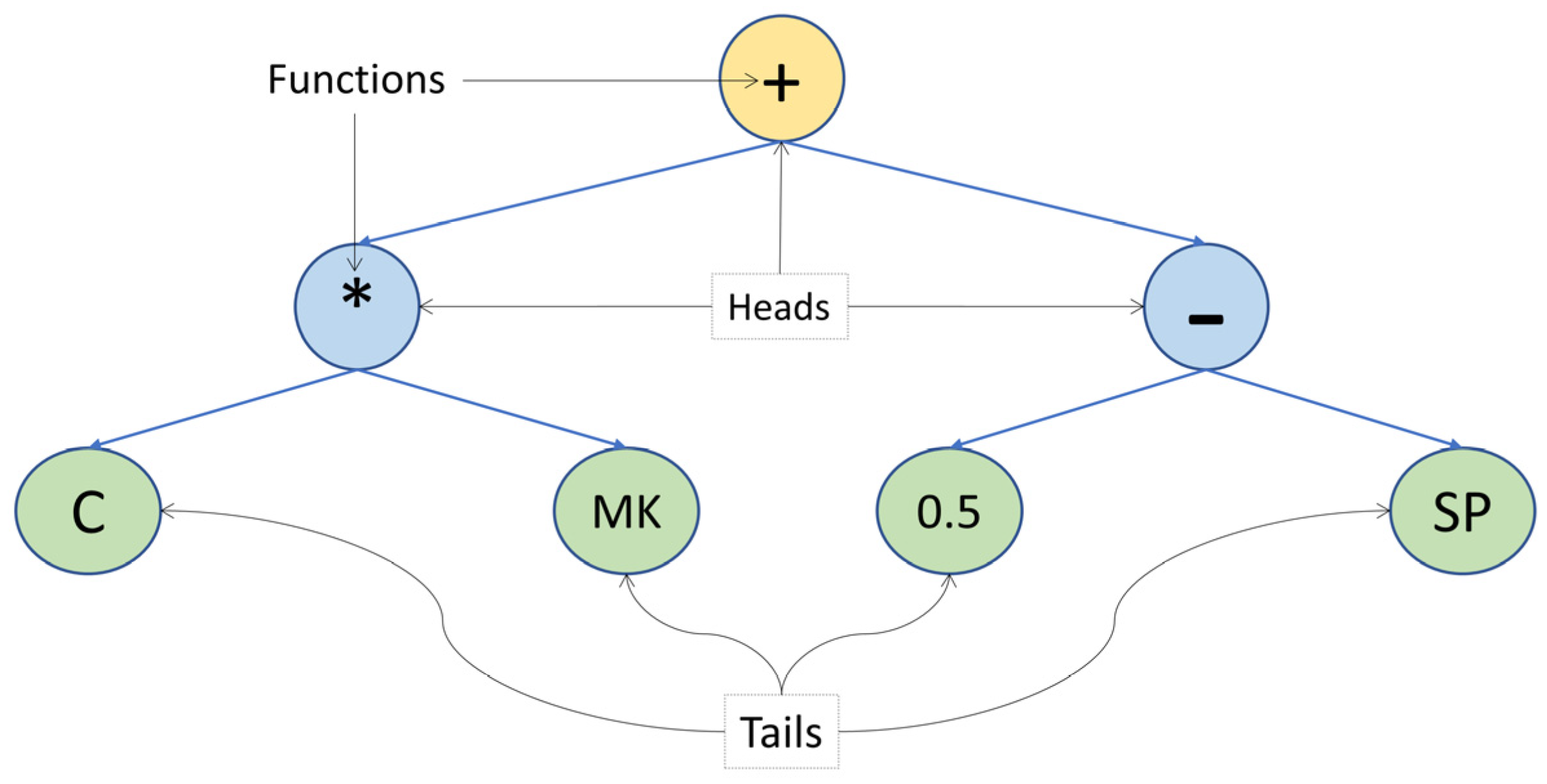
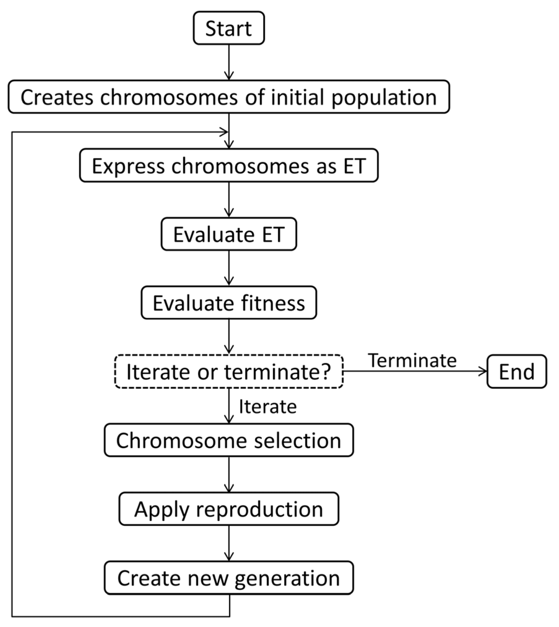
3.1. Gene Expression Programming
3.2. Artificial Neural Network
3.3. M5P Model Tree Algorithm
3.4. Random Forest
4. Model Development and Evaluation Criteria
5. Results and Discussion
5.1. Developed Models for Compressive Strength
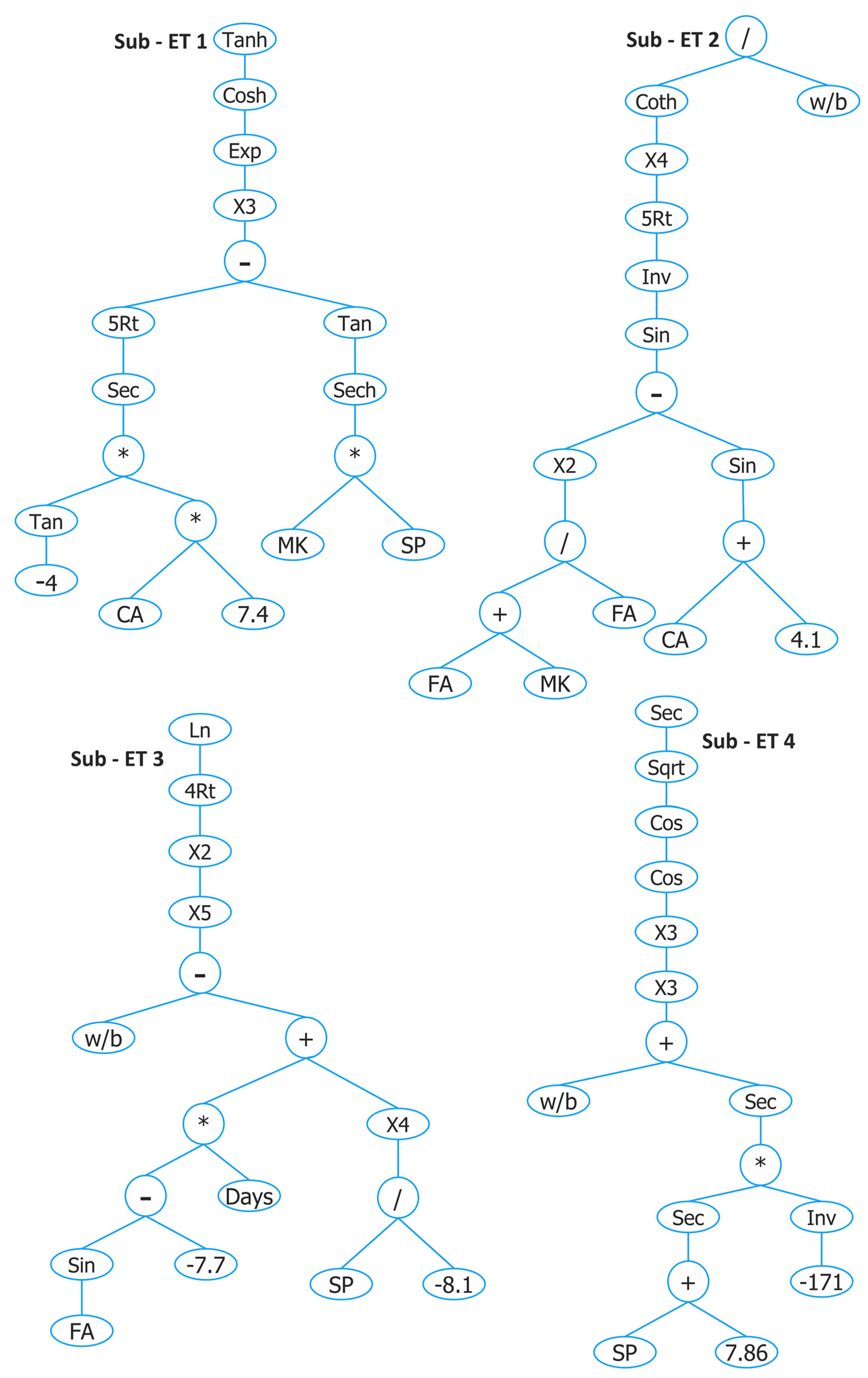
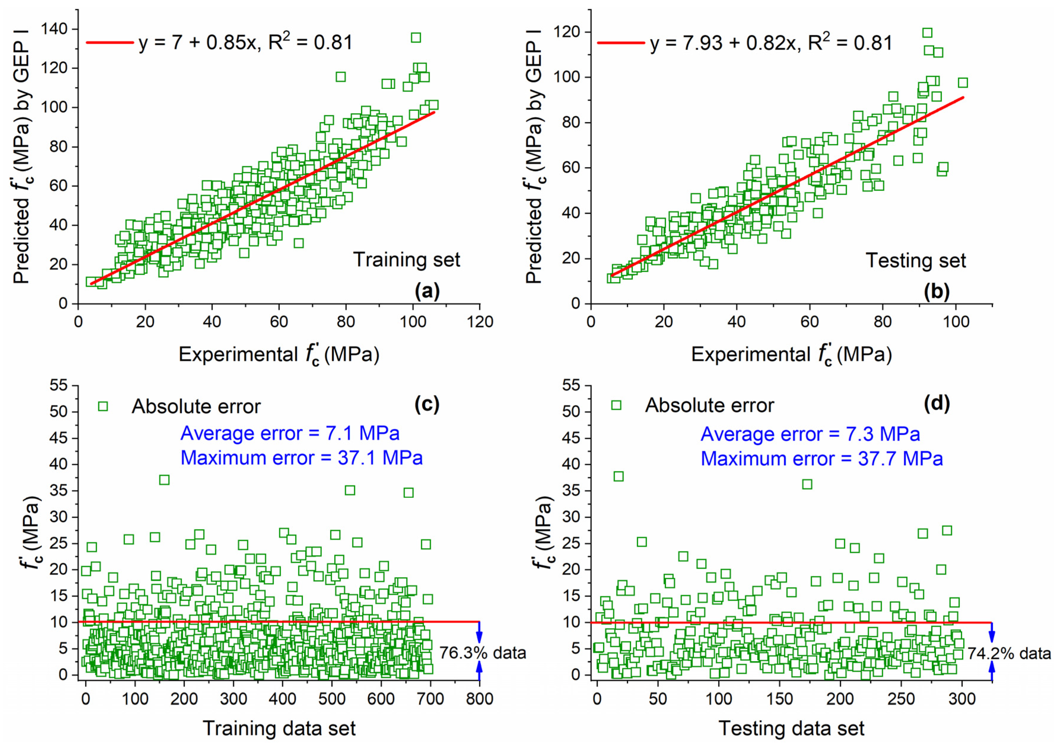
5.1.1. GEP I Model
5.1.2. ANN I Model
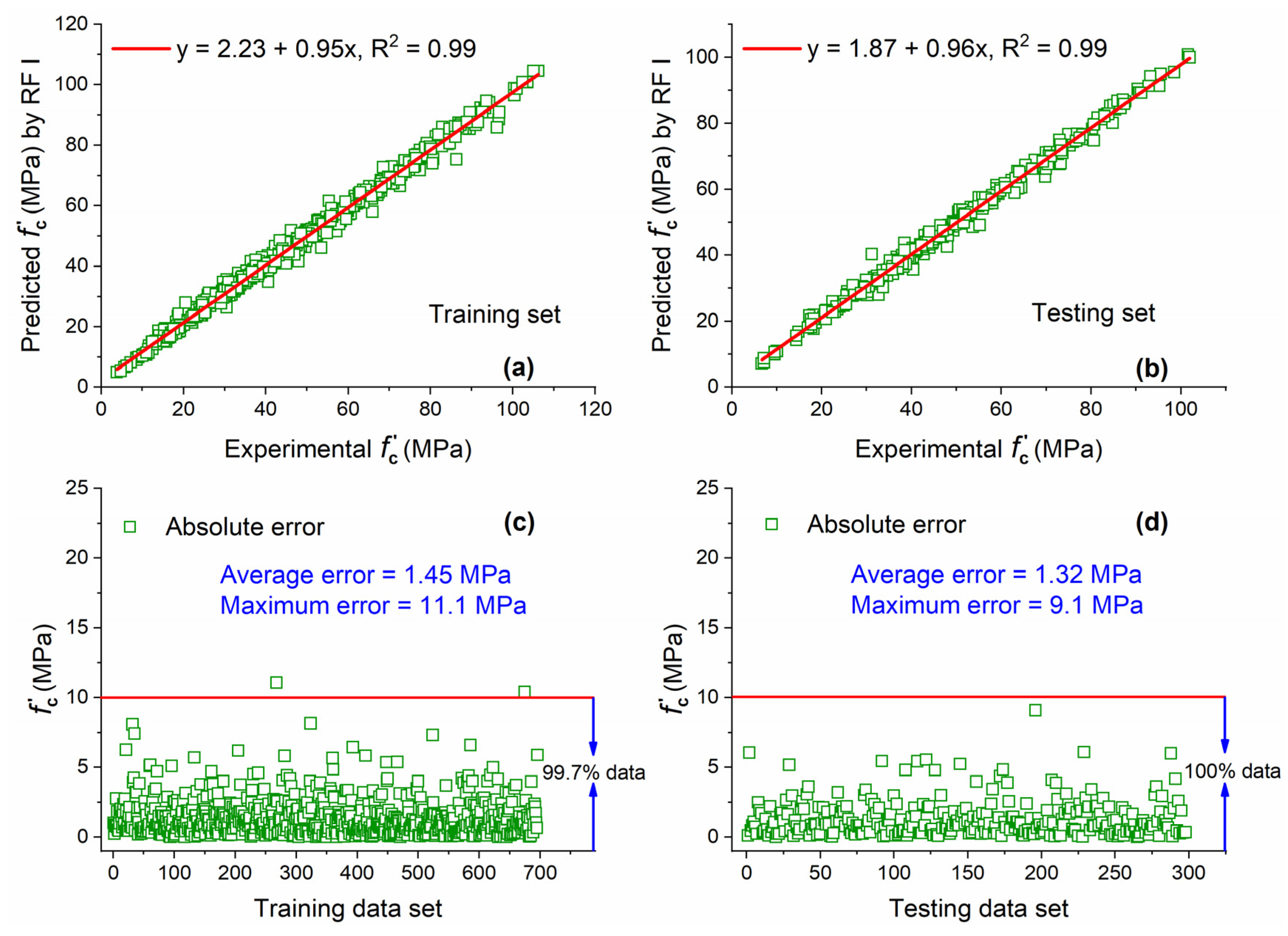
5.1.3. RF I
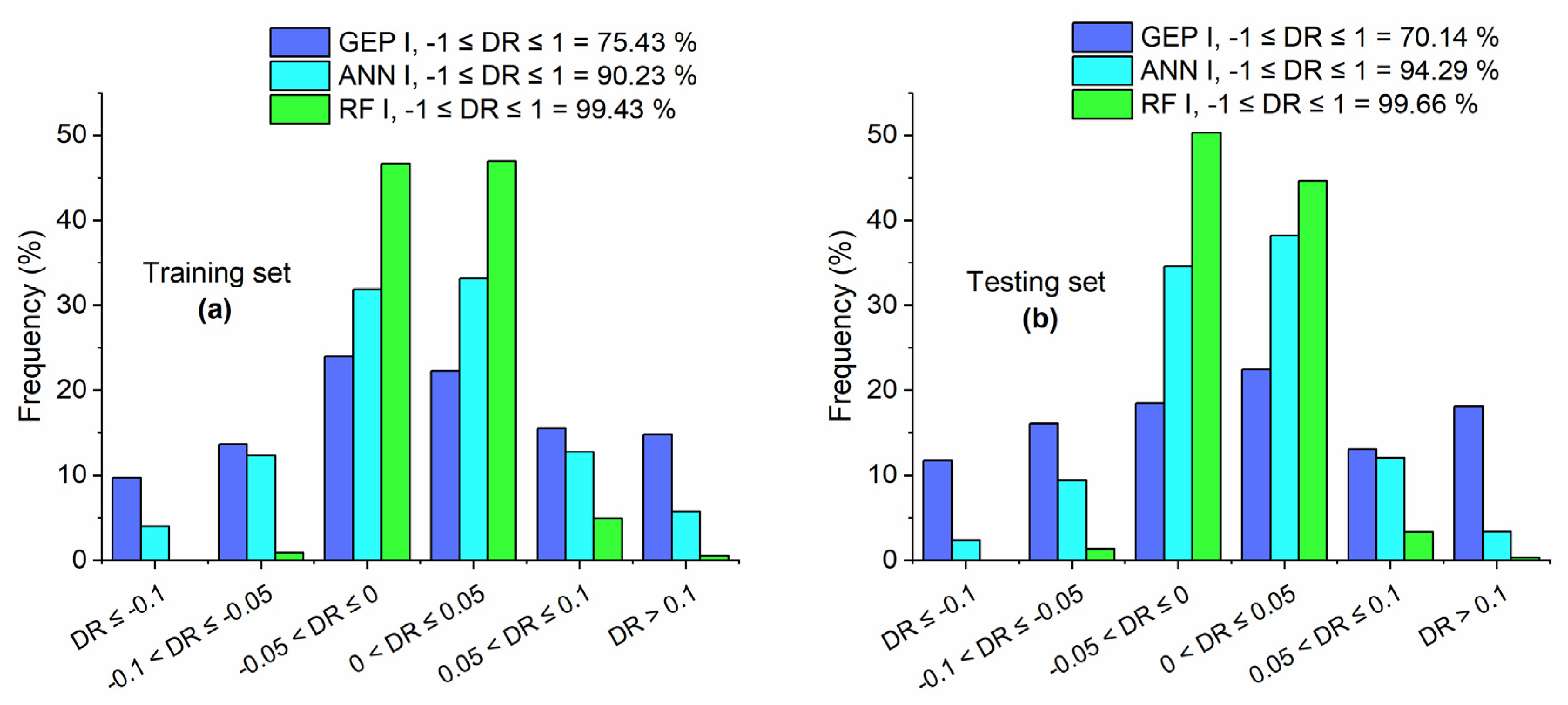
5.1.4. Comparison of GEP I, ANN I, and RF I
5.2. Developed Models for Splitting Tensile Strength
5.2.1. GEP II
5.2.2. ANN II
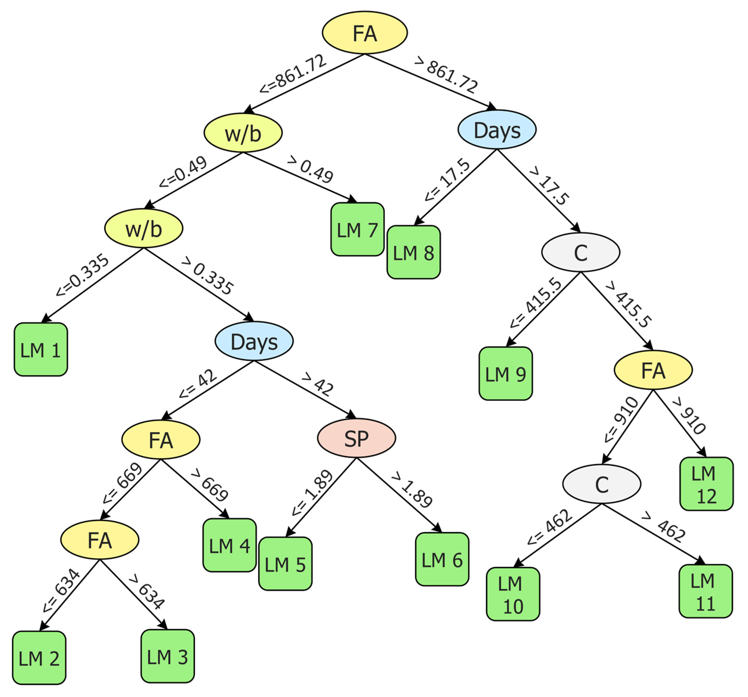
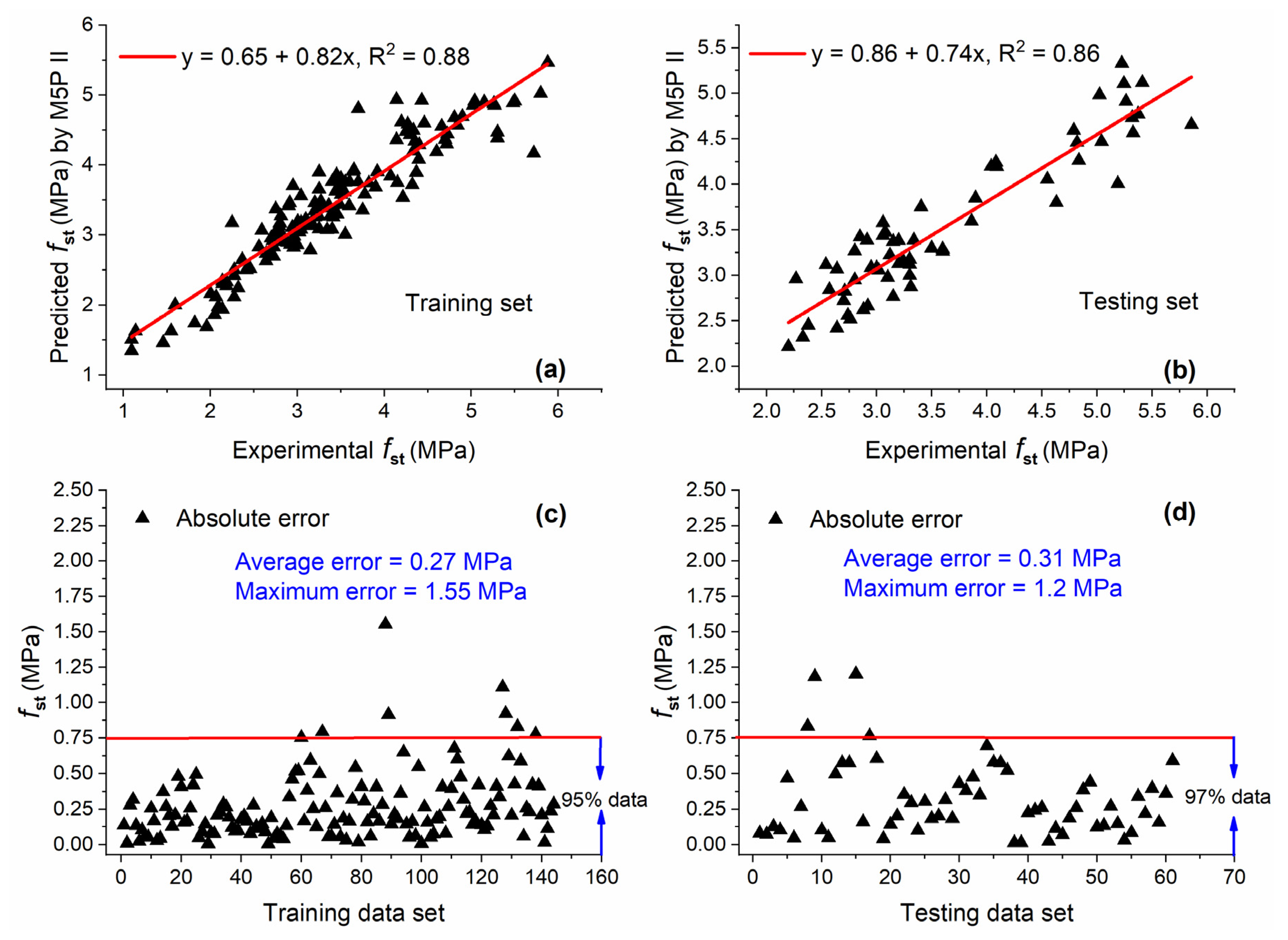
5.2.3. M5P II
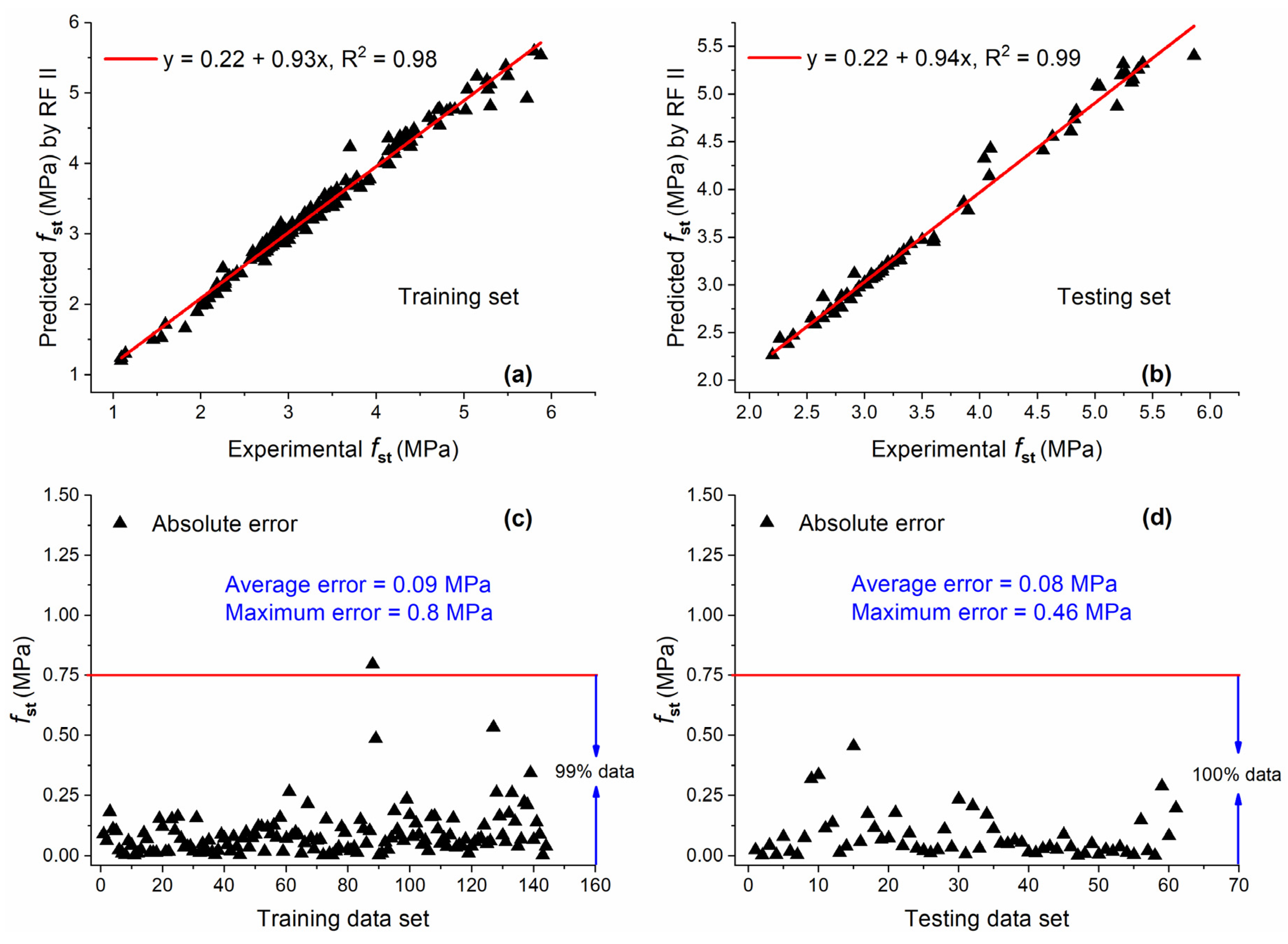
5.2.4. RF II
5.2.5. Comparison of GEP II, ANN II, M5P II, and RF II
5.3. Developed Models for Flexural Strength
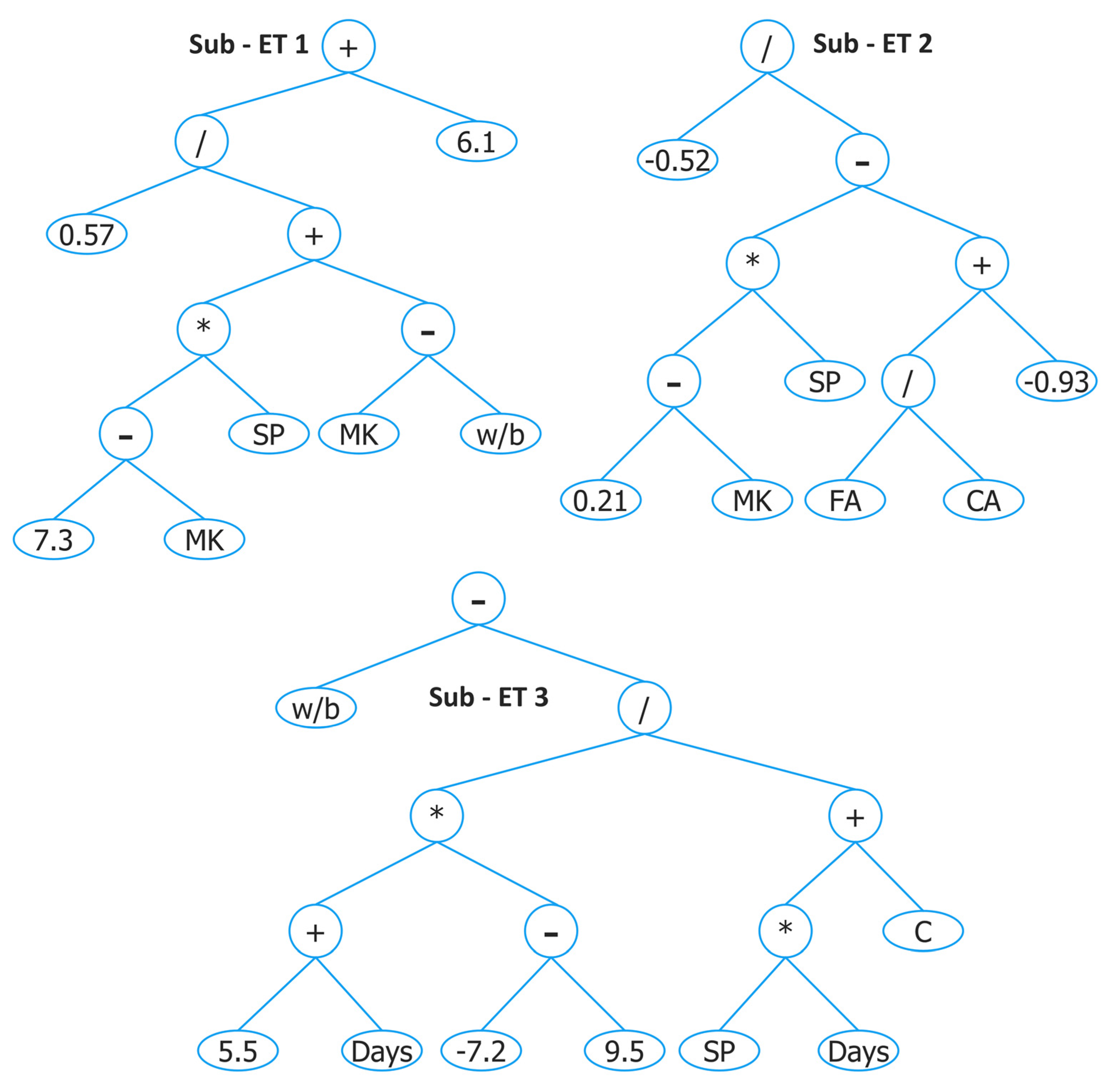
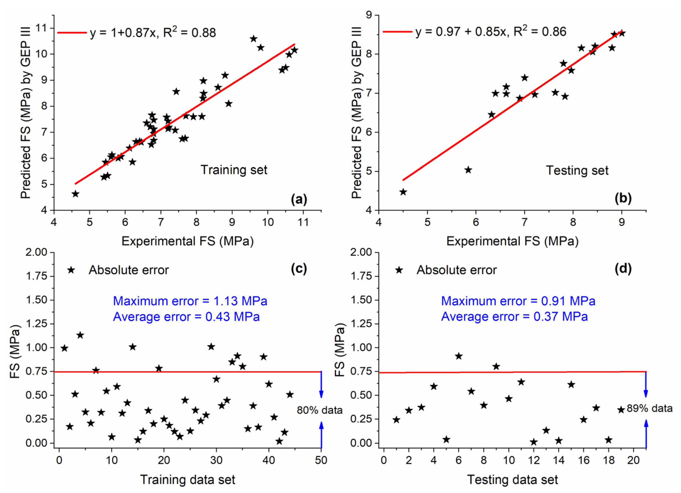
5.3.1. GEP III
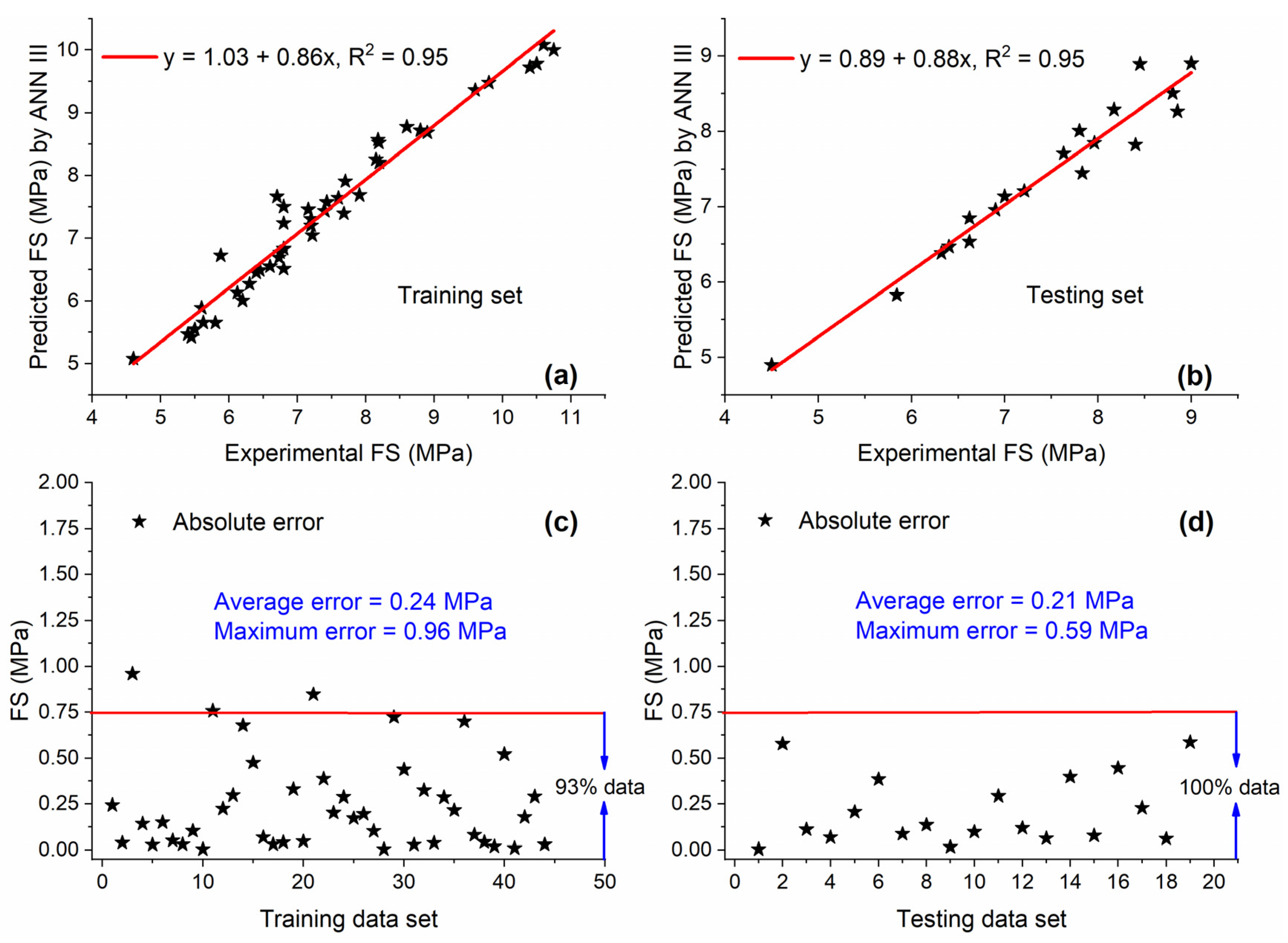
5.3.2. ANN III
5.3.3. M5P III
5.3.4. RF III
5.3.5. Comparison of GEP III, ANN III, M5P III, and RF III
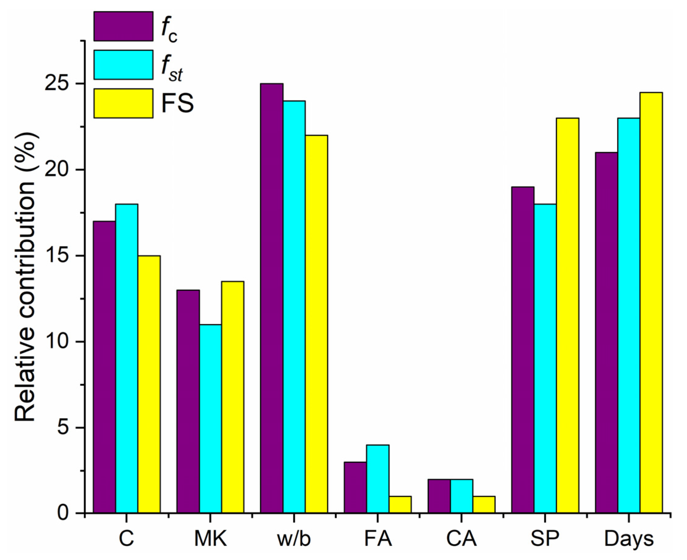
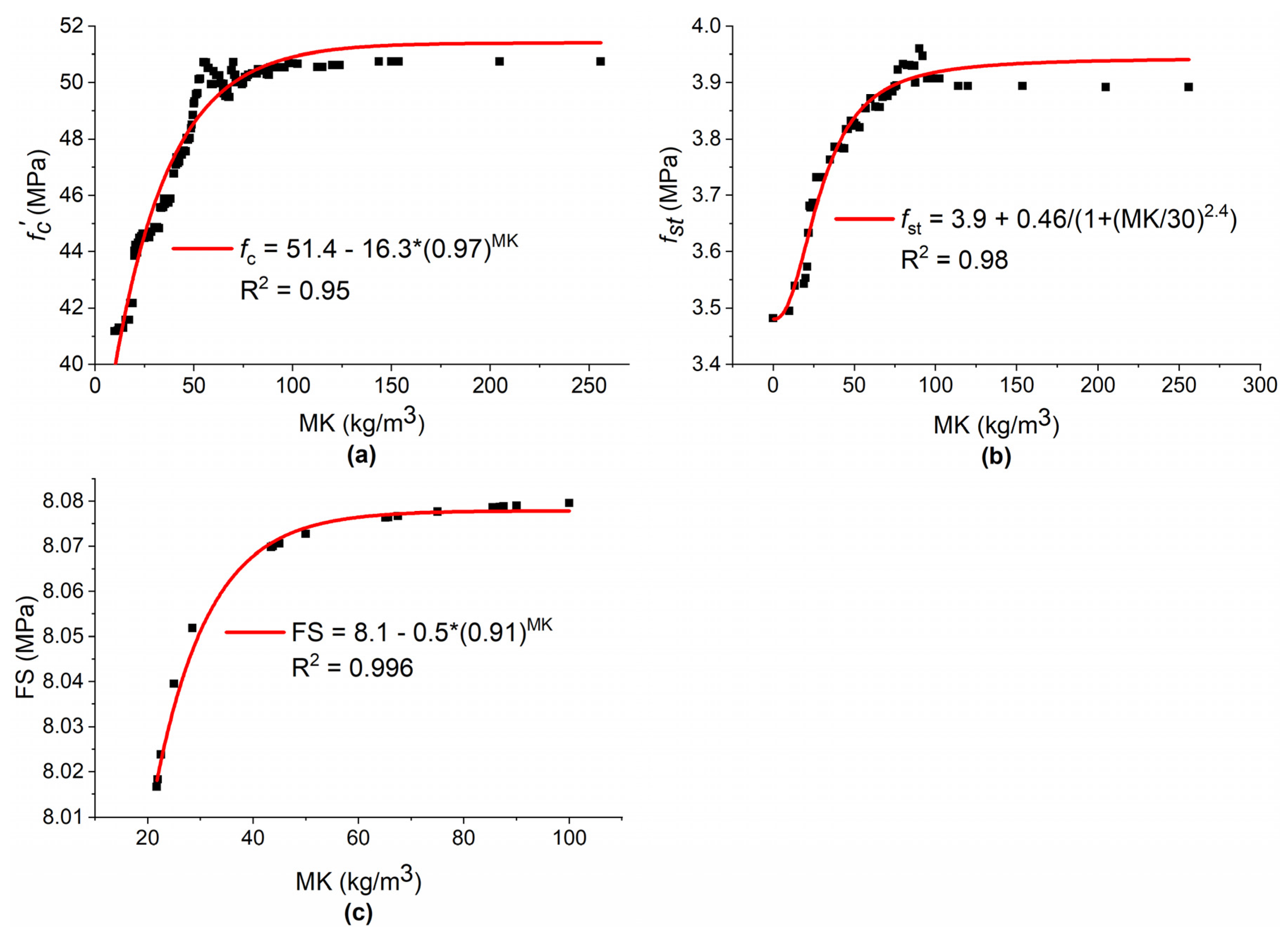
6. Sensitivity and Parametric Analysis
7. Conclusions
- For modelling of concrete with MK, RF I (R2 = 0.99) showed excellent predictive capability followed by ANN I (R2 = 0.94) and GEP I (R2 = 0.81) for both training and testing sets. These results were also supported by other statistical metrics such as R, RMSE, RSE, MAE, DR, and .
- For the training set, in the case of the prediction, RF II performed better with R2 = 0.98 followed by ANN II (R2 = 0.92), M5P II (R2 = 0.88), and GEP II (R2 = 0.86). A slight change was observed in the order of ML techniques in the case of the testing set, where GEP II (R2 = 0.90) performed well as compared with M5P II (R2 = 0.86), while the order of RF II and ANN III was the same as observed for the training set.
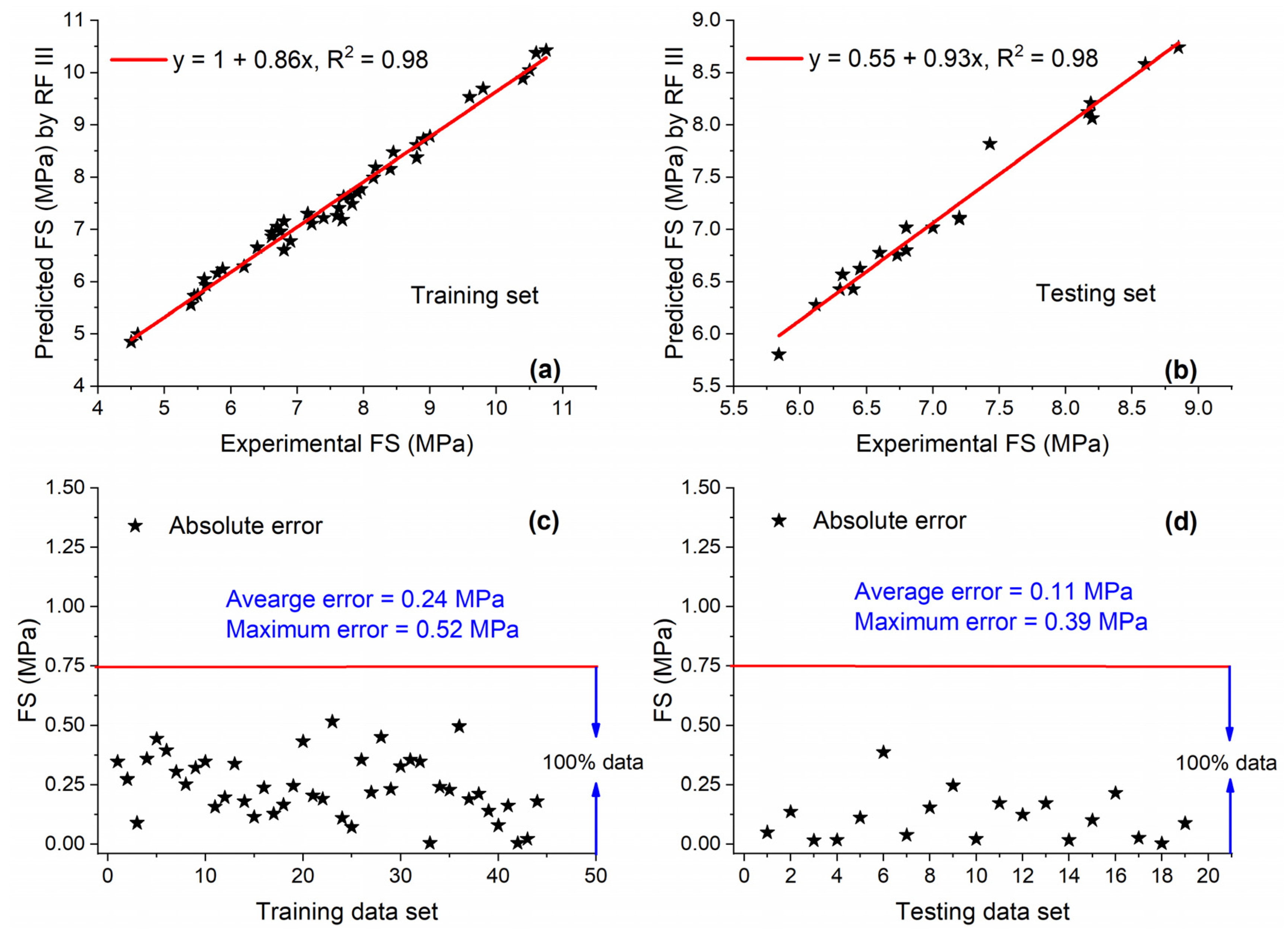
- Similar to the prediction results of and database, RF III remained on top with respect to its excellent prediction performance as compared with other ML techniques for the FS database. The values of R2 equal to 0.98 and 0.98 were observed by RF III and ANN III for both training and testing sets. For the FS database, M5P III’s performance was relatively low as compared with other ML techniques and showed R2 = 0.73 and 0.76 for training and testing sets, respectively. GEP III showed better prediction potential as compared with M5P III with R2 = 0.88 and 0.86 for training and testing sets, respectively.
- PA analysis showed that 15% MK incorporation as partial cement replacement was suitable for both and , while this content was 10% for FS. In addition, significant strength development was observed at early ages with MK incorporation for all the mechanical properties.
8. Future Research
- In this study, four individual machine learning techniques were used for predicting the mechanical properties of concrete with MK. It would be beneficial to use the ensemble ML technique and compare it with individual ML techniques.
- More properties of concrete with MK such as rheology, elastic modulus, and durability characteristics need to be modelled by using advanced ML techniques.
Supplementary Materials
Author Contributions
Funding
Data Availability Statement
Conflicts of Interest
References
- Coninck, H.; Loos, M.; Metz, B.; Davidson, O.; Meyer, L. IPCC Special Report on Carbon Dioxide Capture and Storage; Intergovernmental Panel on Climate Change: Geneva, Switzerland, 2005. [Google Scholar]
- Yang, K.-H.; Song, J.-K.; Song, K.-I. Assessment of CO2 reduction of alkali-activated concrete. J. Clean. Prod. 2013, 39, 265–272. [Google Scholar] [CrossRef]
- Taylor, M.; Tam, C.; Gielen, D. Energy efficiency and CO2 emissions from the global cement industry. Korea 2006, 50, 61–67. [Google Scholar]
- Lenka, S.; Panda, K. Effect of metakaolin on the properties of conventional and self compacting concrete. Adv. Concr. Constr. 2017, 5, 31. [Google Scholar] [CrossRef]
- He, C.; Osbaeck, B.; Makovicky, E. Pozzolanic reactions of six principal clay minerals: Activation, reactivity assessments and technological effects. Cem. Concr. Res. 1995, 25, 1691–1702. [Google Scholar] [CrossRef]
- Siddique, R.; Klaus, J. Influence of metakaolin on the properties of mortar and concrete: A review. Appl. Clay Sci. 2009, 43, 392–400. [Google Scholar] [CrossRef]
- Bredy, P.; Chabannet, M.; Pera, J. Microstructure and porosity of metakaolin blended cements. MRS Online Proc. Libr. 1988, 136, 275–280. [Google Scholar] [CrossRef]
- Khatib, J.; Wild, S. Pore size distribution of metakaolin paste. Cem. Concr. Res. 1996, 26, 1545–1553. [Google Scholar] [CrossRef]
- Brooks, J.; Johari, M.M. Effect of metakaolin on creep and shrinkage of concrete. Cem. Concr. Compos. 2001, 23, 495–502. [Google Scholar] [CrossRef]
- Li, Z.; Ding, Z. Property improvement of Portland cement by incorporating with metakaolin and slag. Cem. Concr. Res. 2003, 33, 579–584. [Google Scholar] [CrossRef]
- Kadri, E.-H.; Kenai, S.; Ezziane, K.; Siddique, R.; De Schutter, G. Influence of metakaolin and silica fume on the heat of hydration and compressive strength development of mortar. Appl. Clay Sci. 2011, 53, 704–708. [Google Scholar] [CrossRef]
- Duan, P.; Shui, Z.; Chen, W.; Shen, C. Effects of metakaolin, silica fume and slag on pore structure, interfacial transition zone and compressive strength of concrete. Constr. Build. Mater. 2013, 44, 1–6. [Google Scholar] [CrossRef]
- Si-Ahmed, M.; Belakrouf, A.; Kenai, S. Influence of metakaolin on the performance of mortars and concretes. Int. J. Civ. Environ. Eng. 2012, 6, 1010–1013. [Google Scholar]
- Oluokun, F.A.; Burdette, E.G.; Deatherage, J.H. Splitting tensile strength and compressive strength relationships at early ages. Mater. J. 1991, 88, 115–121. [Google Scholar]
- Madandoust, R.; Mousavi, S.Y. Fresh and hardened properties of self-compacting concrete containing metakaolin. Constr. Build. Mater. 2012, 35, 752–760. [Google Scholar] [CrossRef]
- Güneyisi, E.; Gesoğlu, M.; Mermerdaş, K. Improving strength, drying shrinkage, and pore structure of concrete using metakaolin. Mater. Struct. 2008, 41, 937–949. [Google Scholar] [CrossRef]
- Dinakar, P.; Sahoo, P.K.; Sriram, G. Effect of metakaolin content on the properties of high strength concrete. Int. J. Concr. Struct. Mater. 2013, 7, 215–223. [Google Scholar] [CrossRef] [Green Version]
- John, N. Strength properties of metakaolin admixed concrete. Int. J. Sci. Res. Publ. 2013, 3, 1–7. [Google Scholar]
- Vu, D.; Stroeven, P.; Bui, V. Strength and durability aspects of calcined kaolin-blended Portland cement mortar and concrete. Cem. Concr. Compos. 2001, 23, 471–478. [Google Scholar] [CrossRef]
- Tawfik, A.; Metwally, K.A.; Zaki, W.; Faried, A.S. Hybrid effect of nanosilica and metakaolin on mechanical properties of cement mortar. Int. J. Eng. Res. Technol. 2019, 8, 2278-0181. [Google Scholar]
- Javed, M.F.; Amin, M.N.; Shah, M.I.; Khan, K.; Iftikhar, B.; Farooq, F.; Aslam, F.; Alyousef, R.; Alabduljabbar, H. Applications of gene expression programming and regression techniques for estimating compressive strength of bagasse ash based concrete. Crystals 2020, 10, 737. [Google Scholar] [CrossRef]
- Azimi-Pour, M.; Eskandari-Naddaf, H. ANN and GEP prediction for simultaneous effect of nano and micro silica on the compressive and flexural strength of cement mortar. Constr. Build. Mater. 2018, 189, 978–992. [Google Scholar] [CrossRef]
- Behnood, A.; Behnood, V.; Gharehveran, M.M.; Alyamac, K.E. Prediction of the compressive strength of normal and high-performance concretes using M5P model tree algorithm. Constr. Build. Mater. 2017, 142, 199–207. [Google Scholar] [CrossRef]
- Erdal, H.; Erdal, M.; Simsek, O.; Erdal, H.I. Prediction of concrete compressive strength using non-destructive test results. Comput. Concr. 2018, 21, 407–417. [Google Scholar]
- Aslam, F.; Farooq, F.; Amin, M.N.; Khan, K.; Waheed, A.; Akbar, A.; Javed, M.F.; Alyousef, R.; Alabdulijabbar, H. Applications of Gene Expression Programming for Estimating Compressive Strength of High-Strength Concrete. Adv. Civ. Eng. 2020, 2020, 8850535. [Google Scholar] [CrossRef]
- Naderpour, H.; Rafiean, A.H.; Fakharian, P. Compressive strength prediction of environmentally friendly concrete using artificial neural networks. J. Build. Eng. 2018, 16, 213–219. [Google Scholar] [CrossRef]
- Getahun, M.A.; Shitote, S.M.; Gariy, Z.C.A. Artificial neural network based modelling approach for strength prediction of concrete incorporating agricultural and construction wastes. Constr. Build. Mater. 2018, 190, 517–525. [Google Scholar] [CrossRef]
- Hadzima-Nyarko, M.; Nyarko, E.K.; Ademović, N.; Miličević, I.; Kalman Šipoš, T. Modelling the influence of waste rubber on compressive strength of concrete by artificial neural networks. Materials 2019, 12, 561. [Google Scholar] [CrossRef] [Green Version]
- Mohammed, A.; Rafiq, S.; Sihag, P.; Kurda, R.; Mahmood, W.; Ghafor, K.; Sarwar, W. ANN, M5P-tree and nonlinear regression approaches with statistical evaluations to predict the compressive strength of cement-based mortar modified with fly ash. J. Mater. Res. Technol. 2020, 9, 12416–12427. [Google Scholar] [CrossRef]
- Ayaz, Y.; Kocamaz, A.F.; Karakoç, M.B. Modeling of compressive strength and UPV of high-volume mineral-admixtured concrete using rule-based M5 rule and tree model M5P classifiers. Constr. Build. Mater. 2015, 94, 235–240. [Google Scholar] [CrossRef]
- Farooq, F.; Nasir Amin, M.; Khan, K.; Rehan Sadiq, M.; Faisal Javed, M.; Aslam, F.; Alyousef, R. A Comparative Study of Random Forest and Genetic Engineering Programming for the Prediction of Compressive Strength of High Strength Concrete (HSC). Appl. Sci. 2020, 10, 7330. [Google Scholar] [CrossRef]
- Mehta, P.K.; Monteiro, P.J. Concrete: Microstructure, Properties, and Materials; McGraw-Hill Education: New York, NY, USA, 2014. [Google Scholar]
- Akin, O.O.; Ocholi, A.; Abejide, O.S.; Obari, J.A. Prediction of the Compressive Strength of Concrete Admixed with Metakaolin Using Gene Expression Programming. Adv. Civ. Eng. 2020, 2020, 8883412. [Google Scholar] [CrossRef]
- Qian, X.; Li, Z. The relationships between stress and strain for high-performance concrete with metakaolin. Cem. Concr. Res. 2001, 31, 1607–1611. [Google Scholar] [CrossRef]
- Poon, C.-S.; Kou, S.; Lam, L. Compressive strength, chloride diffusivity and pore structure of high performance metakaolin and silica fume concrete. Constr. Build. Mater. 2006, 20, 858–865. [Google Scholar] [CrossRef]
- Ramezanianpour, A.; Jovein, H.B. Influence of metakaolin as supplementary cementing material on strength and durability of concretes. Constr. Build. Mater. 2012, 30, 470–479. [Google Scholar] [CrossRef]
- Khatib, J. Metakaolin concrete at a low water to binder ratio. Constr. Build. Mater. 2008, 22, 1691–1700. [Google Scholar] [CrossRef]
- Gill, A.S.; Siddique, R. Strength and micro-structural properties of self-compacting concrete containing metakaolin and rice husk ash. Constr. Build. Mater. 2017, 157, 51–64. [Google Scholar] [CrossRef]
- El-Din, H.K.S.; Eisa, A.S.; Aziz, B.H.A.; Ibrahim, A. Mechanical performance of high strength concrete made from high volume of Metakaolin and hybrid fibers. Constr. Build. Mater. 2017, 140, 203–209. [Google Scholar] [CrossRef]
- Rashad, A.M. A preliminary study on the effect of fine aggregate replacement with metakaolin on strength and abrasion resistance of concrete. Constr. Build. Mater. 2013, 44, 487–495. [Google Scholar] [CrossRef]
- Siddique, R.; Kadri, E.-H. Effect of metakaolin and foundry sand on the near surface characteristics of concrete. Constr. Build. Mater. 2011, 25, 3257–3266. [Google Scholar] [CrossRef]
- Wang, G.; Kong, Y.; Shui, Z.; Li, Q.; Han, J. Experimental investigation on chloride diffusion and binding in concrete containing metakaolin. Corros. Eng. Sci. Technol. 2014, 49, 282–286. [Google Scholar] [CrossRef]
- Dinakar, P.; Manu, S. Concrete mix design for high strength self-compacting concrete using metakaolin. Mater. Des. 2014, 60, 661–668. [Google Scholar] [CrossRef]
- Kavitha, O.; Shanthi, V.; Arulraj, G.P.; Sivakumar, P. Fresh, micro-and macrolevel studies of metakaolin blended self-compacting concrete. Appl. Clay Sci. 2015, 114, 370–374. [Google Scholar] [CrossRef]
- Muduli, R.; Mukharjee, B.B. Effect of incorporation of metakaolin and recycled coarse aggregate on properties of concrete. J. Clean. Prod. 2019, 209, 398–414. [Google Scholar] [CrossRef]
- Joshaghani, A.; Moeini, M.A.; Balapour, M. Evaluation of incorporating metakaolin to evaluate durability and mechanical properties of concrete. Adv. Concr. Constr. 2017, 5, 241. [Google Scholar]
- Badogiannis, E.; Tsivilis, S.; Papadakis, V.; Chaniotakis, E. The effect of metakaolin on concrete properties. In Proceedings of the International Congress on Challenges of Concrete Construction In Innovation and Development in Concrete Materials and Construction, Scotland, UK, 9–11 September 2002; pp. 81–89. [Google Scholar]
- Saand, A.; Keerio, M.A.; Bangwar, D.K. Effect of soorh metakaolin on concrete compressive strength and durability. Eng. Technol. Appl. Sci. Res. 2017, 7, 2210–2214. [Google Scholar] [CrossRef]
- Narmatha, M.; Felixkala, T. Analyse the mechanical properties of metakaolin using as a partial replacement of cement in concrete. Int. J. Adv. Res. Ideas Innov. Technol. 2017, 3, 25–30. [Google Scholar]
- Badogiannis, E.; Tsivilis, S. Exploitation of poor Greek kaolins: Durability of metakaolin concrete. Cem. Concr. Compos. 2009, 31, 128–133. [Google Scholar] [CrossRef]
- Bonakdar, A.; Bakhshi, M.; Ghalibafian, M. Properties of High-performance Concrete ContainingHigh Reactivity Metakaolin. In Proceedings of the 7th International Symposium on Utilization of High-Strength/High-Performance Concrete, Washington, DC, USA, 1 January 2005; pp. 228–295. [Google Scholar]
- Güneyisi, E.; Gesoğlu, M.; Karaoğlu, S.; Mermerdaş, K. Strength, permeability and shrinkage cracking of silica fume and metakaolin concretes. Constr. Build. Mater. 2012, 34, 120–130. [Google Scholar] [CrossRef]
- Kannan, V. Strength and durability performance of self compacting concrete containing self-combusted rice husk ash and metakaolin. Constr. Build. Mater. 2018, 160, 169–179. [Google Scholar] [CrossRef]
- Poon, C.; Kou, S.; Lam, L. Pore size distribution of high performance metakaolin concrete. J. Wuhan Univ. Technol.-Mater. Sci. Ed. 2002, 17, 42–46. [Google Scholar] [CrossRef]
- Meddah, M.S.; Ismail, M.A.; El-Gamal, S.; Fitriani, H. Performances evaluation of binary concrete designed with silica fume and metakaolin. Constr. Build. Mater. 2018, 166, 400–412. [Google Scholar] [CrossRef]
- Ferreira, R.; Castro-Gomes, J.; Costa, P.; Malheiro, R. Effect of metakaolin on the chloride ingress properties of concrete. KSCE J. Civ. Eng. 2016, 20, 1375–1384. [Google Scholar] [CrossRef]
- Shafiq, N.; Nuruddin, M.F.; Khan, S.U.; Ayub, T. Calcined kaolin as cement replacing material and its use in high strength concrete. Constr. Build. Mater. 2015, 81, 313–323. [Google Scholar] [CrossRef]
- Dubey, S.; Chandak, R.; Yadav, R. Experimental study of concrete with metakaolin as partial replacement of OPC. Int. J. Adv. Eng. Res. Sci. 2015, 2, 38–40. [Google Scholar]
- Kannan, V.; Ganesan, K. Chloride and chemical resistance of self compacting concrete containing rice husk ash and metakaolin. Constr. Build. Mater. 2014, 51, 225–234. [Google Scholar] [CrossRef]
- Akcay, B.; Tasdemir, M.A. Performance evaluation of silica fume and metakaolin with identical finenesses in self compacting and fiber reinforced concretes. Constr. Build. Mater. 2018, 185, 436–444. [Google Scholar] [CrossRef]
- Bumanis, G.; Bajare, D.; Korjakins, A. Durability of high strength self compacting concrete with metakaolin containing waste. In Key Engineering Materials; Trans Tech Publications Ltd.: Zurich, Switzerland, 2016; pp. 65–70. [Google Scholar]
- Ofuyatan, O.M.; Olowofoyeku, A.M.; Edeki, S.; Oluwafemi, J.; Ajao, A.; David, O. Incorporation of silica fume and metakaolin on self compacting concrete. J. Phys. Conf. Ser. 2019, 1378, 042089. [Google Scholar] [CrossRef] [Green Version]
- Ženíšek, M.; Vlach, T.; Laiblová, L. Dosage of Metakaolin in high performance concrete. In Key Engineering Materials; Trans Tech Publications Ltd.: Zurich, Switzerland, 2017; pp. 311–315. [Google Scholar]
- Abouhussien, A.A.; Hassan, A.A. Application of statistical analysis for mixture design of high-strength self-consolidating concrete containing metakaolin. J. Mater. Civ. Eng. 2014, 26, 04014016. [Google Scholar] [CrossRef]
- Sharbatdar, M.K.; Abbasi, M.; Fakharian, P. Improving the properties of self-compacted concrete with using combined silica fume and metakaolin. Period. Polytech. Civ. Eng. 2020, 64, 535–544. [Google Scholar] [CrossRef] [Green Version]
- Güneyisi, E.; Gesoğlu, M. Properties of self-compacting mortars with binary and ternary cementitious blends of fly ash and metakaolin. Mater. Struct. 2008, 41, 1519–1531. [Google Scholar] [CrossRef]
- Kesavraman, S. Studies on Metakaolin based banana fibre reinforced concrete. Int. J. Civ. Eng. Technol. 2017, 8, 532–543. [Google Scholar]
- Al-Oran, A.A.A.; Safiee, N.A.; Nasir, N.A.M. Fresh and hardened properties of self-compacting concrete using metakaolin and GGBS as cement replacement. Eur. J. Environ. Civ. Eng. 2019, 26, 379–392. [Google Scholar] [CrossRef]
- Salimi, J.; Ramezanianpour, A.M.; Moradi, M.J. Studying the effect of low reactivity metakaolin on free and restrained shrinkage of high performance concrete. J. Build. Eng. 2020, 28, 101053. [Google Scholar] [CrossRef]
- Zoe, Y.; Hanif, I.; Adzmier, H.; Eyzati, H.; Syuhaili, M.N. Strength of Self-Compacting Concrete Containing Metakaolin and Nylon Fiber. In IOP Conference Series: Earth and Environmental Science; IOP Publishing: Bristol, UK, 2020; p. 012047. [Google Scholar]
- Kannan, V.; Ganesan, K. Mechanical properties of self-compacting concrete with binary and ternary cementitious blends of metakaolin and fly ash. J. S. Afr. Inst. Civ. Eng. 2014, 56, 97–105. [Google Scholar]
- Kannan, V.; Ganesan, K. Evaluation of mechanical and permeability related properties of self compacting concrete containing metakaolin. Sci. Res. Essays 2012, 7, 4081–4091. [Google Scholar]
- Güneyisi, E.; Gesoğlu, M.; Qays, M.A.; Mermerdaş, K.; İpek, S. Fracture properties of high strength metakaolin and silica fume concretes. In Proceedings of the 3rd International Conference on Chemical, Civil and Environmental Engineering (CCEE-2016), Antalya, Turkey, 20–21 April 2016. [Google Scholar]
- Yi, S.-T.; Yang, E.-I.; Choi, J.-C. Effect of specimen sizes, specimen shapes, and placement directions on compressive strength of concrete. Nucl. Eng. Des. 2006, 236, 115–127. [Google Scholar] [CrossRef]
- Che, Y.; Zhang, N.; Yang, F.; Prafulla, M. Splitting tensile strength of selfconsolidating concrete and its size effect. In Proceedings of the 2016 World Congress (Structures 16), Jeju island, Korea, 28 Augest–1 September 2016. [Google Scholar]
- Kadleček, V.; Modrý, S. Size effect of test specimens on tensile splitting strength of concrete: General relation. Mater. Struct. 2002, 35, 28–34. [Google Scholar] [CrossRef]
- Ferreira, C. Gene expression programming: A new adaptive algorithm for solving problems. Complex Syst. 2001, 13, 87–129. [Google Scholar]
- Sarıdemir, M. Genetic programming approach for prediction of compressive strength of concretes containing rice husk ash. Constr. Build. Mater. 2010, 24, 1911–1919. [Google Scholar] [CrossRef]
- Shah, H.A.; Rehman, S.K.U.; Javed, M.F.; Iftikhar, Y. Prediction of compressive and splitting tensile strength of concrete with fly ash by using gene expression programming. Struct. Concr. 2021. [Google Scholar] [CrossRef]
- Shahmansouri, A.A.; Yazdani, M.; Ghanbari, S.; Bengar, H.A.; Jafari, A.; Ghatte, H.F. Artificial neural network model to predict the compressive strength of eco-friendly geopolymer concrete incorporating silica fume and natural zeolite. J. Clean. Prod. 2020, 279, 123697. [Google Scholar] [CrossRef]
- Liu, Q.-f.; Iqbal, M.F.; Yang, J.; Lu, X.-y.; Zhang, P.; Rauf, M. Prediction of chloride diffusivity in concrete using artificial neural network: Modelling and performance evaluation. Constr. Build. Mater. 2020, 268, 121082. [Google Scholar] [CrossRef]
- Topcu, I.B.; Sarıdemir, M. Prediction of properties of waste AAC aggregate concrete using artificial neural network. Comput. Mater. Sci. 2007, 41, 117–125. [Google Scholar] [CrossRef]
- Quinlan, J.R. Learning with continuous classes. In Proceedings of the 5th Australian Joint Conference on Artificial Intelligence, Singapore, 16–18 November 1992; pp. 343–348. [Google Scholar]
- Wang, Y.; Witten, I.H. Induction of model trees for predicting continuous classes. In Working Paper 96/23; University of Waikato: Hamilton, New Zealand, 1996. [Google Scholar]
- Almasi, S.N.; Bagherpour, R.; Mikaeil, R.; Ozcelik, Y.; Kalhori, H. Predicting the building stone cutting rate based on rock properties and device pullback amperage in quarries using M5P model tree. Geotech. Geol. Eng. 2017, 35, 1311–1326. [Google Scholar] [CrossRef]
- Breiman, L. Random forests. Mach. Learn. 2001, 45, 5–32. [Google Scholar] [CrossRef] [Green Version]
- Breiman, L. Bagging predictors. Mach. Learn. 1996, 24, 123–140. [Google Scholar] [CrossRef] [Green Version]
- Bertsimas, D.; Dunn, J. Optimal classification trees. Mach. Learn. 2017, 106, 1039–1082. [Google Scholar] [CrossRef]
- Sarıdemir, M. Effect of specimen size and shape on compressive strength of concrete containing fly ash: Application of genetic programming for design. Mater. Des. (1980–2015) 2014, 56, 297–304. [Google Scholar] [CrossRef]
- Gandomi, A.H.; Alavi, A.H.; Mirzahosseini, M.R.; Nejad, F.M. Nonlinear genetic-based models for prediction of flow number of asphalt mixtures. J. Mater. Civ. Eng. 2011, 23, 248–263. [Google Scholar] [CrossRef]
- Shahmansouri, A.A.; Bengar, H.A.; Ghanbari, S. Compressive strength prediction of eco-efficient GGBS-based geopolymer concrete using GEP method. J. Build. Eng. 2020, 31, 101326. [Google Scholar] [CrossRef]
- Özcan, F. Gene expression programming based formulations for splitting tensile strength of concrete. Constr. Build. Mater. 2012, 26, 404–410. [Google Scholar] [CrossRef]
- Nazari, A.; Riahi, S. Prediction split tensile strength and water permeability of high strength concrete containing TiO2 nanoparticles by artificial neural network and genetic programming. Compos. Part B Eng. 2011, 42, 473–488. [Google Scholar] [CrossRef]
- Yu, Y.; Nguyen, T.N.; Li, J.; Sanchez, L.F.; Nguyen, A. Predicting elastic modulus degradation of alkali silica reaction affected concrete using soft computing techniques: A comparative study. Constr. Build. Mater. 2021, 274, 122024. [Google Scholar] [CrossRef]
- Khan, M.A.; Memon, S.A.; Farooq, F.; Javed, M.F.; Aslam, F.; Alyousef, R. Compressive Strength of Fly-Ash-Based Geopolymer Concrete by Gene Expression Programming and Random Forest. Adv. Civ. Eng. 2021, 2021, 6618407. [Google Scholar] [CrossRef]
- Gandomi, A.H.; Yun, G.J.; Alavi, A.H. An evolutionary approach for modeling of shear strength of RC deep beams. Mater. Struct. 2013, 46, 2109–2119. [Google Scholar] [CrossRef]
- Curcio, F.; DeAngelis, B.; Pagliolico, S. Metakaolin as a pozzolanic microfiller for high-performance mortars. Cem. Concr. Res. 1998, 28, 803–809. [Google Scholar] [CrossRef]
- Poon, C.-S.; Lam, L.; Kou, S.; Wong, Y.-L.; Wong, R. Rate of pozzolanic reaction of metakaolin in high-performance cement pastes. Cem. Concr. Res. 2001, 31, 1301–1306. [Google Scholar] [CrossRef]
- Bai, J.; Wild, S.; Gailius, A. Accelerating early strength development of concrete using metakaolin as an admixture. Mater. Sci. 2004, 10, 338–344. [Google Scholar]


| Statistical Indicator | C (kg/m3) | MK (kg/m3) | w/b Ratio | FA (kg/m3) | CA (kg/m3) | SP (kg/m3) | Days | Strength (MPa) |
|---|---|---|---|---|---|---|---|---|
| Database | ||||||||
| Minimum | 176.25 | 0 | 0.21 | 272.5 | 0 | 0 | 1 | 4 |
| Maximum | 680 | 256 | 0.8 | 1502 | 1510 | 24 | 180 | 107 |
| Mean | 384.77 | 44.35 | 0.447 | 765 | 991 | 3.6 | 36 | 48.86 |
| Standard error | 2.8 | 1.15 | 0.004 | 5.95 | 8.88 | 0.125 | 1.4 | 0.73 |
| Standard deviation | 87 | 36.26 | 0.124 | 186.3 | 278.33 | 3.91 | 44.54 | 22.85 |
| Kurtosis | −0.13 | 3.59 | 0.45 | 3.29 | 2.3 | 7.44 | 3.83 | −0.435 |
| Skewness | 0.03 | 1.1 | 0.73 | 1.14 | −1.3 | 2.16 | 2.07 | 0.48 |
| Database | ||||||||
| Minimum | 266 | 0 | 0.21 | 272.5 | 175.1 | 0 | 1 | 1.1 |
| Maximum | 570 | 256 | 0.75 | 989 | 1265 | 12.4 | 120 | 5.88 |
| Mean | 400 | 44.1 | 0.44 | 756 | 866 | 4.23 | 34.62 | 3.44 |
| Standard error | 4.59 | 2.72 | 0.008 | 12.63 | 18.64 | 0.23 | 2.21 | 0.071 |
| Standard deviation | 65.69 | 39 | 0.12 | 180.83 | 267 | 3.34 | 31.67 | 1.01 |
| Kurtosis | −0.36 | 4.2 | −0.005 | −0.39 | 1.6 | −0.68 | 0.37 | −0.25 |
| Skewness | 0.14 | 1.31 | 0.41 | −0.58 | −1.11 | 0.41 | 1.23 | 0.42 |
| FS Database | ||||||||
| Minimum | 304 | 0 | 0.28 | 624.8 | 822 | 0 | 7 | 4.5 |
| Maximum | 570 | 100 | 0.48 | 843 | 1265 | 8.55 | 90 | 10.75 |
| Mean | 399.5 | 44.22 | 0.415 | 716 | 1051 | 1.97 | 39.98 | 7.38 |
| Standard error | 7.21 | 4.04 | 0.006 | 11.44 | 20.7 | 0.24 | 3.89 | 0.18 |
| Standard deviation | 57.21 | 32.05 | 0.051 | 90.83 | 164.5 | 1.94 | 30.89 | 1.42 |
| Kurtosis | 0.59 | −1.31 | 1.024 | −1.61 | −1.3 | 0.92 | −0.95 | 0.055 |
| Skewness | 0.31 | 0.03 | −1.085 | 0.5 | −0.22 | 1.01 | 0.74 | 0.461 |
| Parameters | GEP I | GEP II | GEP III |
|---|---|---|---|
| Genes | 4 | 5 | 3 |
| Head size | 13 | 10 | 8 |
| Chromosomes | 50 | 30 | 250 |
| Function set | +, −, ∗, /, Sqrt, Exp, Ln, Inv, X2, X3, X4, X5, 4Rt, 5Rt, Sin, Cos, Tan, Sec, Cosh, Tanh, Coth, Sech | +, −, ∗, /, Sqrt, Exp, Ln, Log, Inv, 3Rt, Cos, Tan, Cot, Sec, Coth, Tanh, Sech | +, −, ∗, / |
| Linking function | Multiplication | Addition | Addition |
| Generation | 400,000 | 70,000 | 50,000 |
| Fitness function error type | RMSE | RMSE | RMSE |
| Mutation rate | 0.00138 | 0.00138 | 0.00138 |
| No. of Chromosomes | Head Size | No. of Genes | Linking Function | Function Set | Output | R2 (Training Set) | R2 (Testing Set) | Ref. |
|---|---|---|---|---|---|---|---|---|
| 30 | 10 | 4 | Addition | +, −, ∗, /, X2, 3Rt | of concrete with bagasse ash | 0.83 | 0.85 | [21] |
| 30 | 10 | 4 | Addition | +, −, ∗, / | of high strength concrete | 0.91 | 0.9 | [25] |
| 26 | 12 | 3 | Multiplication | +, −, ∗, /, Sqrt, X3 | of geopolymer concrete with blast-furnace slag | 0.92 | 0.94 | [91] |
| 20 | 4 | 2 | Multiplication | +, −, ∗, /, Sqrt | and w/b | 0.87 | 0.88 | [92] |
| Model | Training Set | Testing Set | ||||||||
|---|---|---|---|---|---|---|---|---|---|---|
| R | RMSE | RRMSE | RSE | R | RMSE | RRMSE | RSE | |||
| GEP I | 0.9 | 9.3 | 0.19 | 0.19 | 0.1 | 0.9 | 9.43 | 0.2 | 0.19 | 0.12 |
| ANN I | 0.97 | 5.49 | 0.12 | 0.063 | 0.061 | 0.97 | 5.18 | 0.1 | 0.063 | 0.051 |
| RF I | 0.997 | 2.03 | 0.044 | 0.01 | 0.02 | 0.996 | 1.86 | 0.04 | 0.01 | 0.02 |
| Models | Coefficients | |||||||
|---|---|---|---|---|---|---|---|---|
| a | b | c | d | e | f | g | h | |
| LM 1 | 5.52 | 0 | −0.0002 | −1.19 | −0.003 | 0 | 0.145 | 0.03 |
| LM 2 | 7.06 | −0.003 | 0.005 | −6.091 | −0.001 | 0.0002 | 0.015 | 0.0214 |
| LM 3 | 5.2 | −0.003 | 0.0037 | −5.55 | 0.0017 | 0.0002 | 0.0151 | 0.0151 |
| LM 4 | 5.78 | −0.005 | 0.0035 | −4.62 | −0.0002 | 0.0015 | 0.0151 | 0.022 |
| LM 5 | 8.08 | −0.0041 | 0.0015 | −8.45 | 0.0006 | 0.0003 | 0.063 | 0.01 |
| LM 6 | 8.4 | −0.004 | 0.0015 | −8.45 | 0.0003 | 0.0003 | 0.074 | 0.01 |
| LM 7 | 3.732 | 0.0016 | 0.004 | −2.3 | −0.0006 | 0 | −0.0053 | 0.011 |
| LM 8 | 9.6 | 0.0025 | 0.0076 | −2.955 | −0.0077 | 0 | −0.049 | 0.0574 |
| LM 9 | 6.9 | 0.0047 | 0.0099 | −2.0359 | −0.0057 | 0 | −0.0404 | 0.0063 |
| LM 10 | 15.8 | 0.0013 | 0.012 | −5.56 | −0.012 | 0 | −0.047 | 0.005 |
| LM 11 | 15.8 | 0.0013 | 0.0119 | −5.56 | −0.012 | 0 | −0.047 | 0.005 |
| LM 12 | 10.57 | 0.0032 | 0.011 | −4.43 | −0.008 | 0 | −0.047 | 0.005 |
| Model | Training Set | Testing Set | ||||||||
|---|---|---|---|---|---|---|---|---|---|---|
| R | RMSE | RRMSE | RSE | R | RMSE | RRMSE | RSE | |||
| GEP II | 0.93 | 0.378 | 0.111 | 0.14 | 0.06 | 0.95 | 0.339 | 0.096 | 0.11 | 0.05 |
| ANN II | 0.96 | 0.2816 | 0.0836 | 0.08 | 0.043 | 0.98 | 0.198 | 0.0548 | 0.04 | 0.03 |
| M5P II | 0.94 | 0.3547 | 0.1053 | 0.12 | 0.05 | 0.93 | 0.4053 | 0.112 | 0.17 | 0.06 |
| RF II | 0.99 | 0.135 | 0.04 | 0.02 | 0.02 | 0.99 | 0.122 | 0.0337 | 0.015 | 0.02 |
| Model | Training Set | Testing Set | ||||||||
|---|---|---|---|---|---|---|---|---|---|---|
| R | RMSE | RRMSE | RSE | R | RMSE | RRMSE | RSE | |||
| GEP III | 0.94 | 0.5326 | 0.07226 | 0.125 | 0.04 | 0.93 | 0.455 | 0.0616 | 0.16 | 0.03 |
| ANN III | 0.98 | 0.3522 | 0.048 | 0.055 | 0.02 | 0.97 | 0.2753 | 0.0373 | 0.06 | 0.02 |
| M5P III | 0.85 | 0.858 | 0.1146 | 0.3 | 0.06 | 0.87 | 0.7054 | 0.099 | 0.66 | 0.05 |
| RF III | 0.99 | 0.247 | 0.0366 | 0.03 | 0.018 | 0.99 | 0.147 | 0.0207 | 0.03 | 0.01 |
Publisher’s Note: MDPI stays neutral with regard to jurisdictional claims in published maps and institutional affiliations. |
© 2022 by the authors. Licensee MDPI, Basel, Switzerland. This article is an open access article distributed under the terms and conditions of the Creative Commons Attribution (CC BY) license (https://creativecommons.org/licenses/by/4.0/).
Share and Cite
Shah, H.A.; Yuan, Q.; Akmal, U.; Shah, S.A.; Salmi, A.; Awad, Y.A.; Shah, L.A.; Iftikhar, Y.; Javed, M.H.; Khan, M.I. Application of Machine Learning Techniques for Predicting Compressive, Splitting Tensile, and Flexural Strengths of Concrete with Metakaolin. Materials 2022, 15, 5435. https://doi.org/10.3390/ma15155435
Shah HA, Yuan Q, Akmal U, Shah SA, Salmi A, Awad YA, Shah LA, Iftikhar Y, Javed MH, Khan MI. Application of Machine Learning Techniques for Predicting Compressive, Splitting Tensile, and Flexural Strengths of Concrete with Metakaolin. Materials. 2022; 15(15):5435. https://doi.org/10.3390/ma15155435
Chicago/Turabian StyleShah, Hammad Ahmed, Qiang Yuan, Usman Akmal, Sajjad Ahmad Shah, Abdelatif Salmi, Youssef Ahmed Awad, Liaqat Ali Shah, Yusra Iftikhar, Muhammad Haris Javed, and Muhammad Imtiaz Khan. 2022. "Application of Machine Learning Techniques for Predicting Compressive, Splitting Tensile, and Flexural Strengths of Concrete with Metakaolin" Materials 15, no. 15: 5435. https://doi.org/10.3390/ma15155435
APA StyleShah, H. A., Yuan, Q., Akmal, U., Shah, S. A., Salmi, A., Awad, Y. A., Shah, L. A., Iftikhar, Y., Javed, M. H., & Khan, M. I. (2022). Application of Machine Learning Techniques for Predicting Compressive, Splitting Tensile, and Flexural Strengths of Concrete with Metakaolin. Materials, 15(15), 5435. https://doi.org/10.3390/ma15155435