
Correlation of Bone Material Model Using Voxel Mesh and Parametric Optimization


Abstract
:1. Introduction
2. Materials and Methods
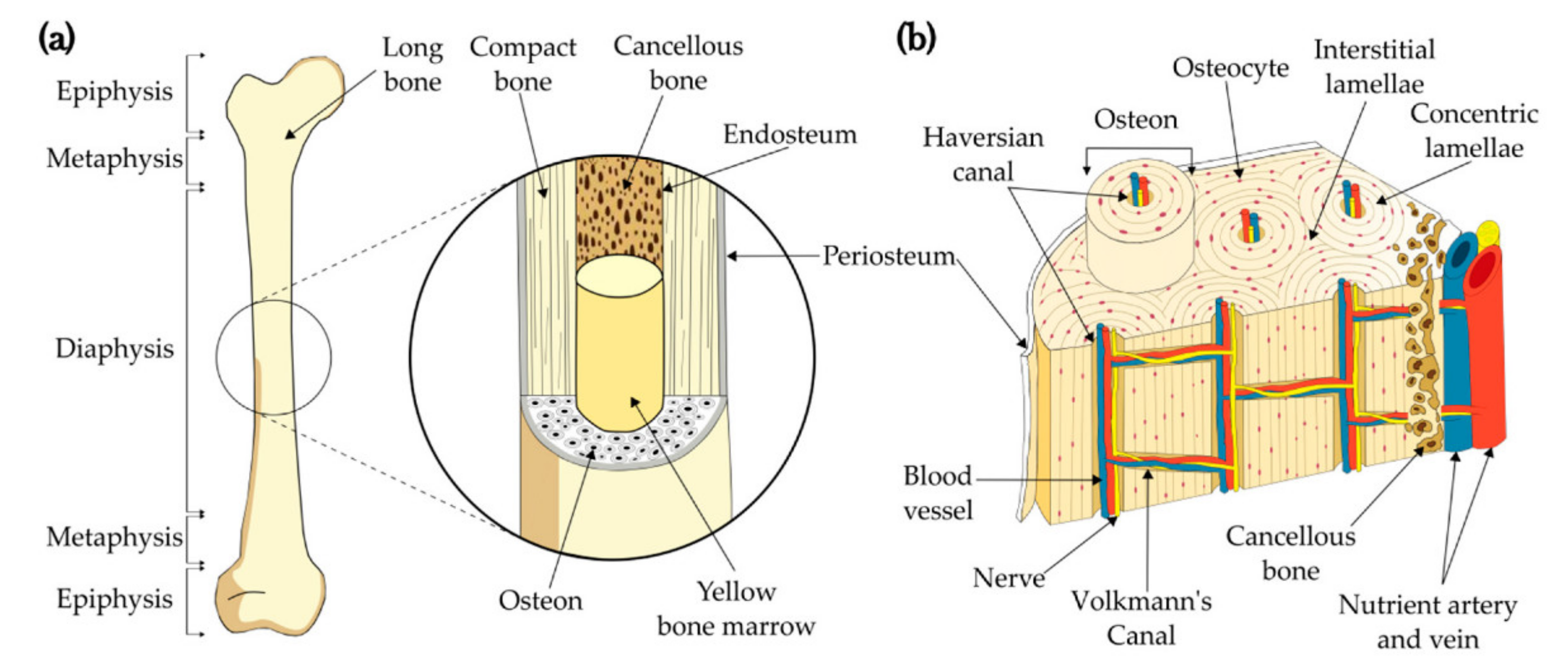
2.1. Analyzed Object
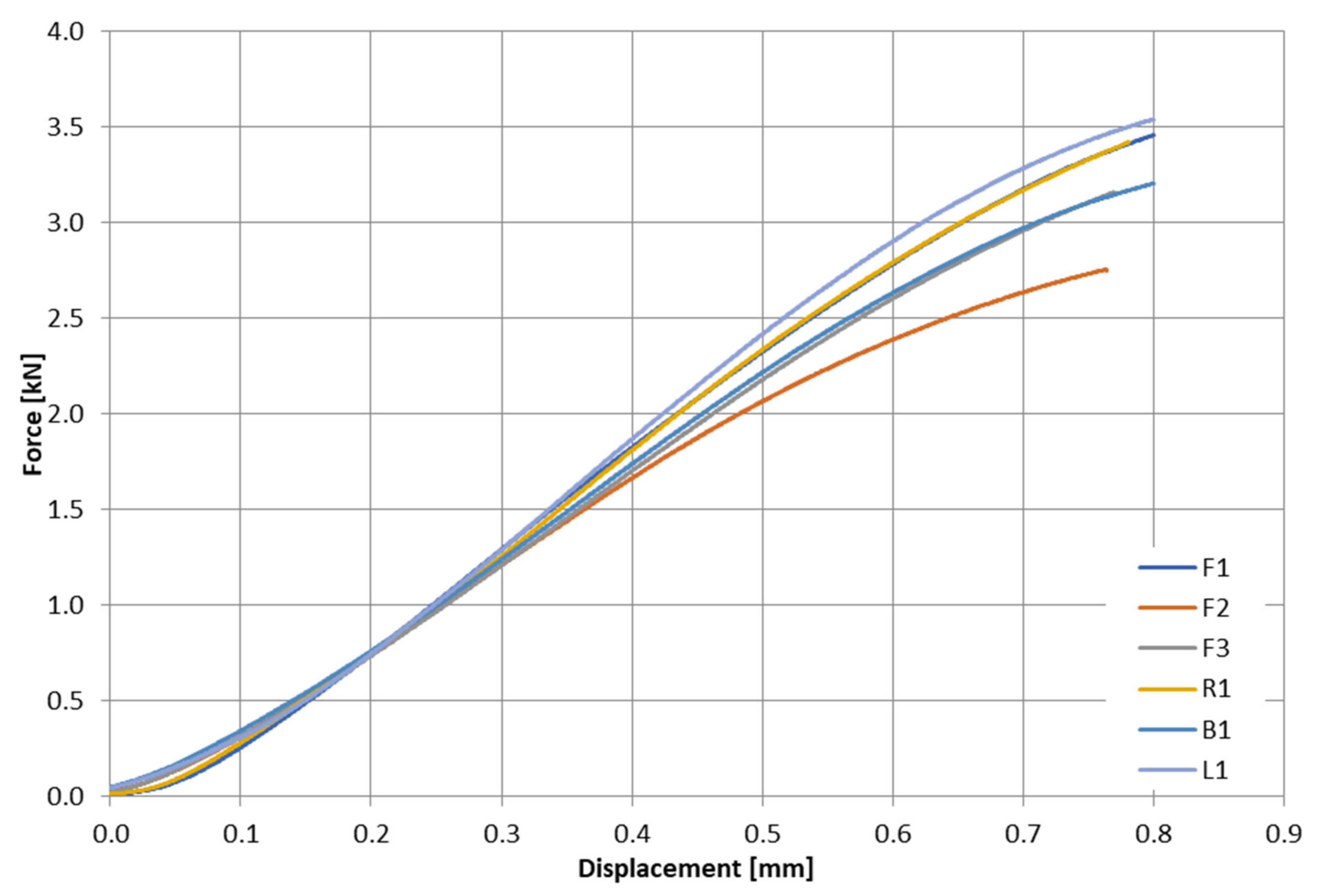
2.2. Experimental Testing
2.3. FE Models Development
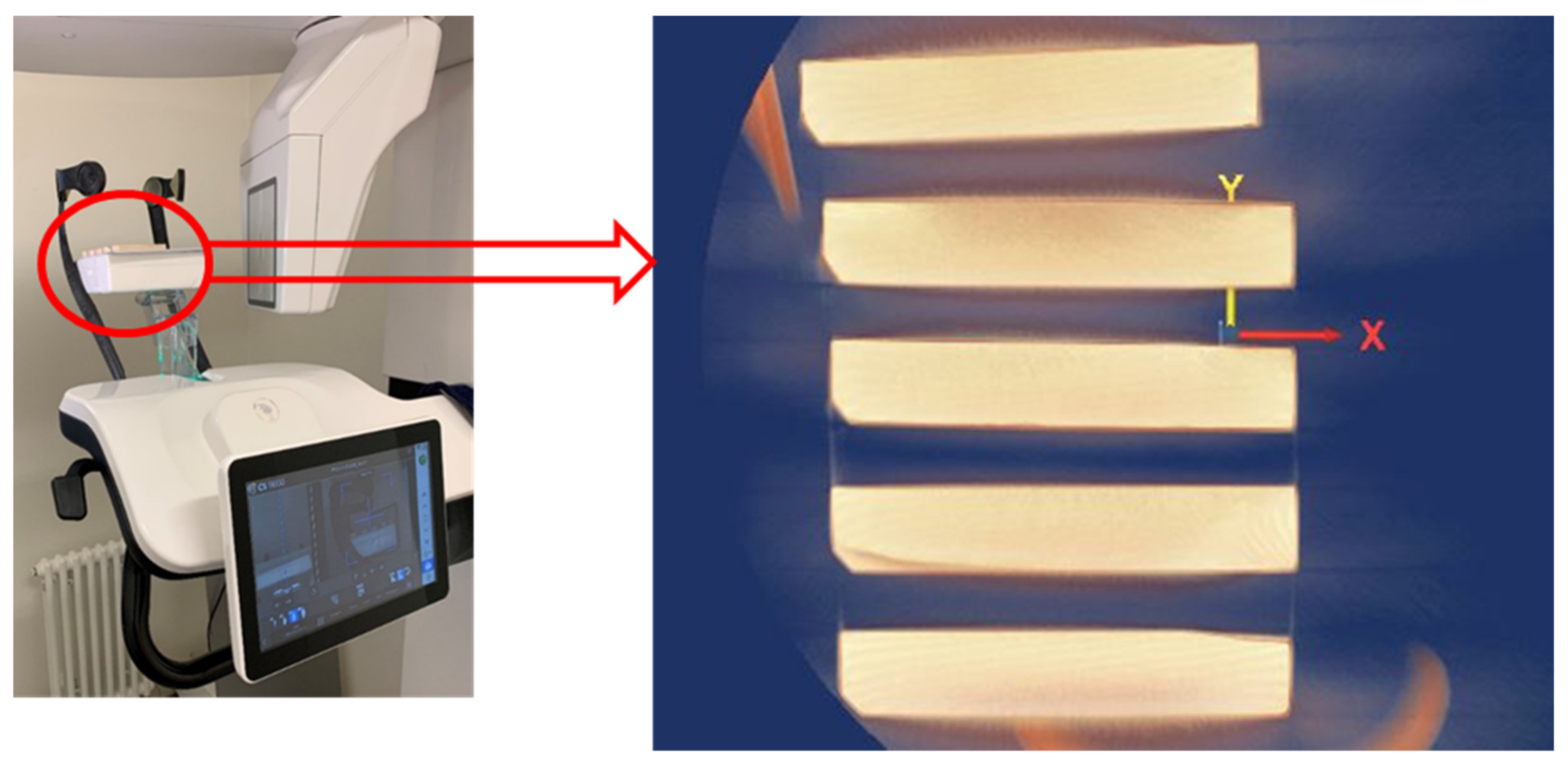
2.3.1. CBCT Imaging
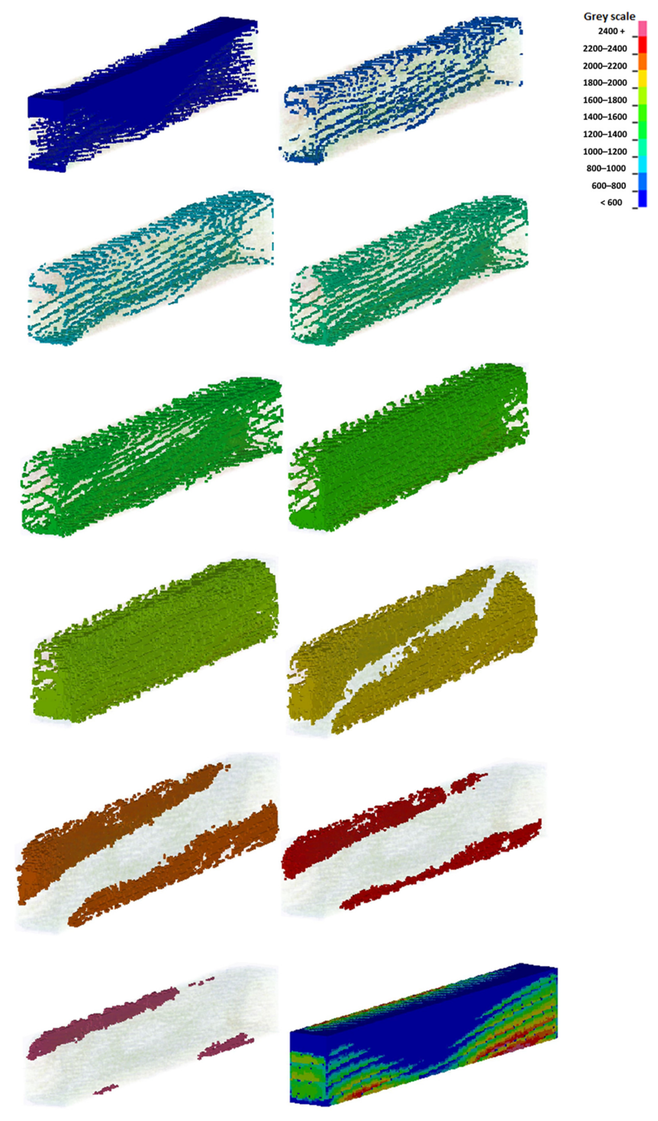
2.3.2. Generation of Voxel Mesh

| Manufacturer | Type | Tube Voltage | Tube Current | Frequency | Tube Focal Spot (IEC 60336) | Total Filtration | Voxel Size |
|---|---|---|---|---|---|---|---|
| Cerastream Dental LLC, Atlanta, GA, USA | CS9600 | 60.0–90.0 kV 60.0–120.0 kV (optional) | 2.0–15.0 mA | 140 kHz | 0.3 mm | >2.5 mm eq. Al | 75.0 µm minimum |
2.4. FE Analysis
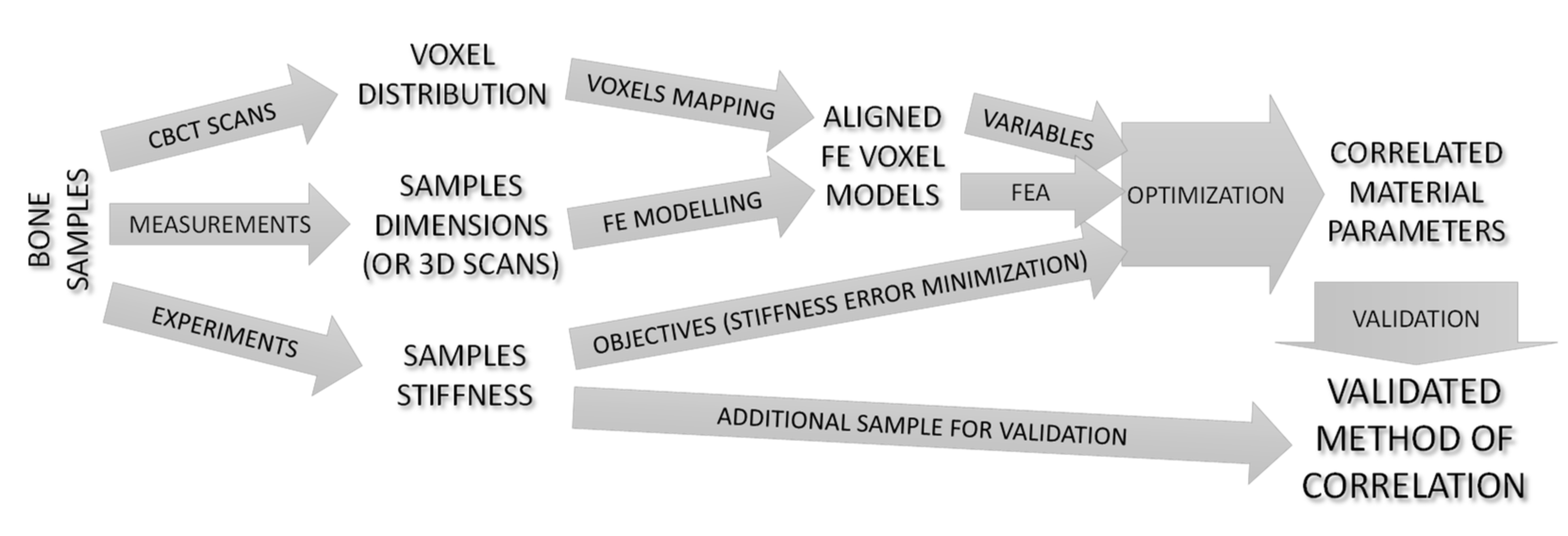
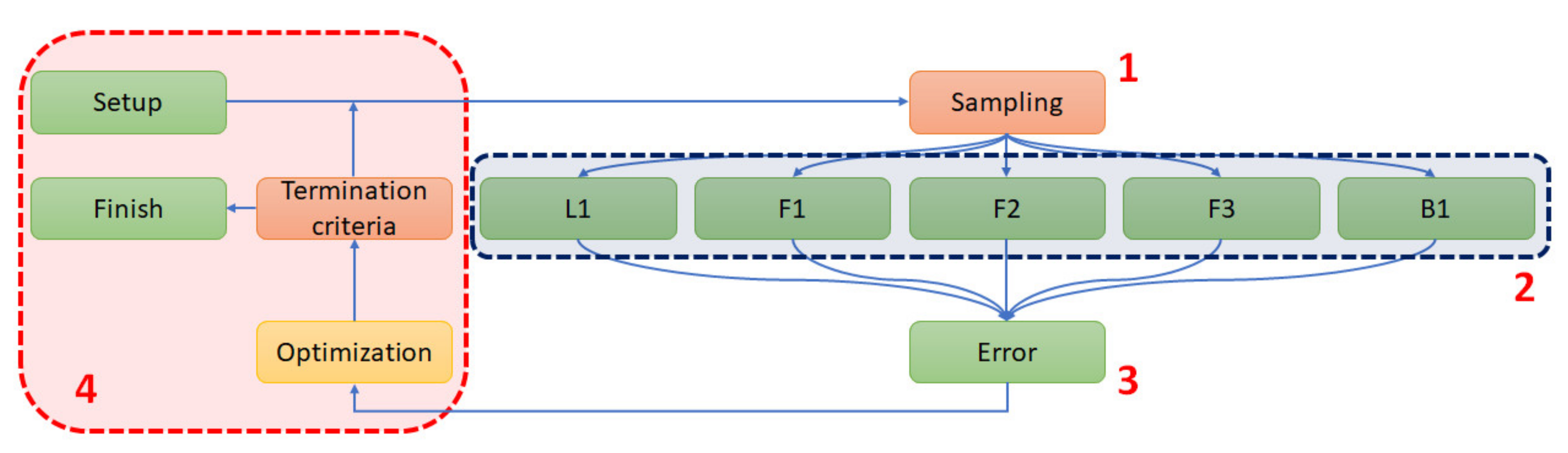
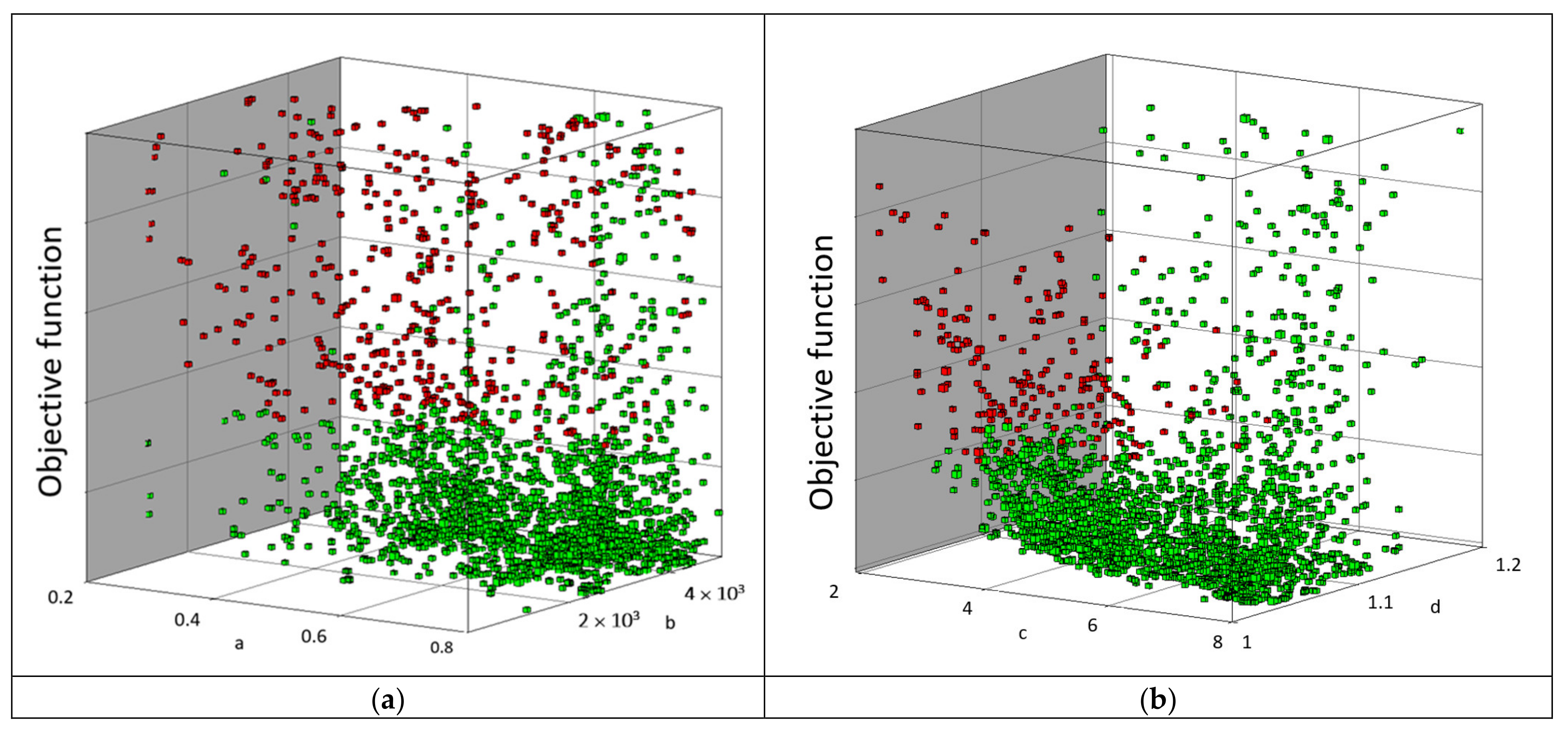
2.5. Parametric Optimization
- (1)
- The sampling of variables;
- (2)
- A parallel numerical analysis of five samples using the Newton–Raphson scheme (analysis);
- (3)
- The acquisition of the force–displacement curves and error norm calculation;
- (4)
- Optimization stage.
3. Results
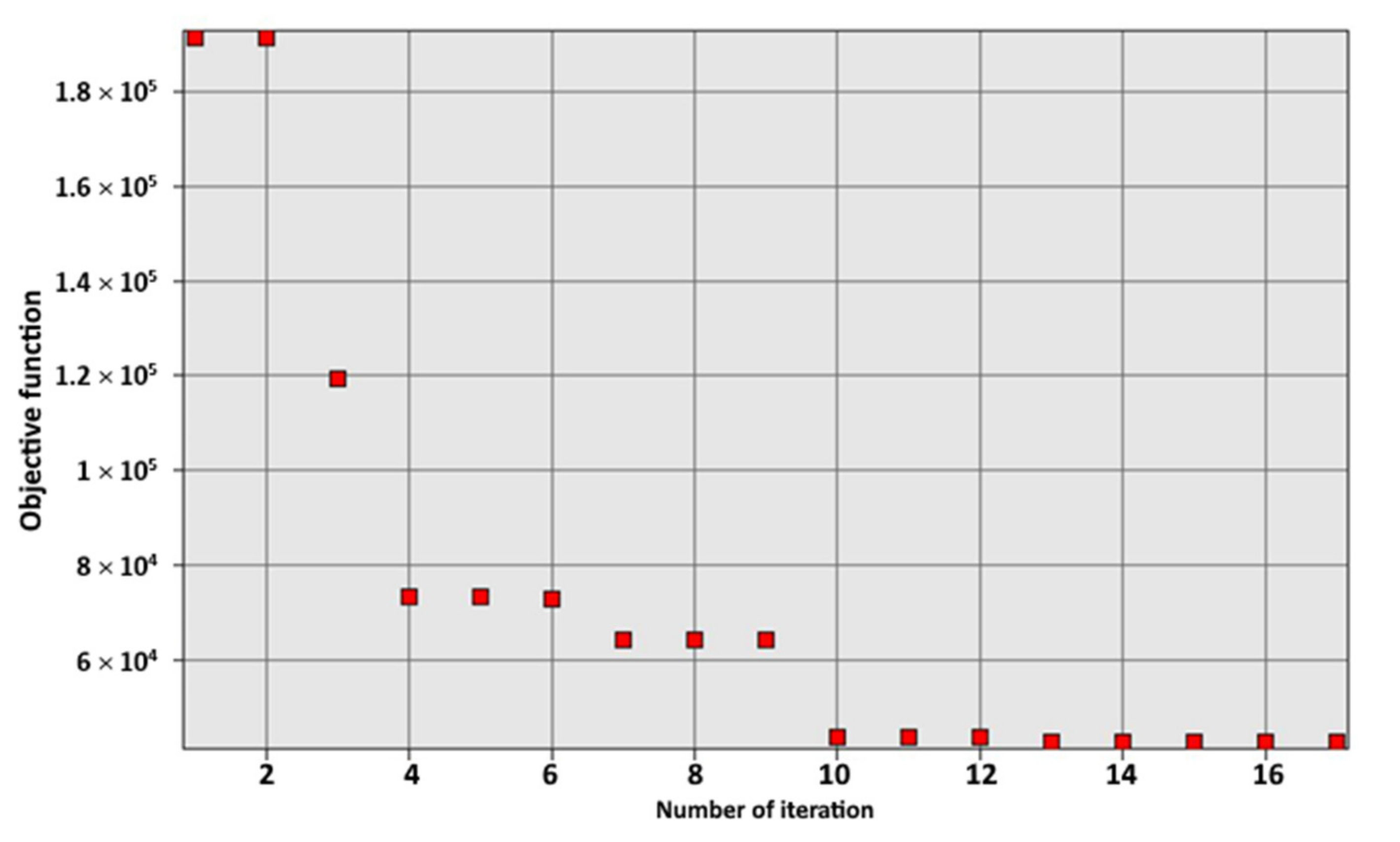
3.1. Optimization
3.2. Method Validation—Step #1
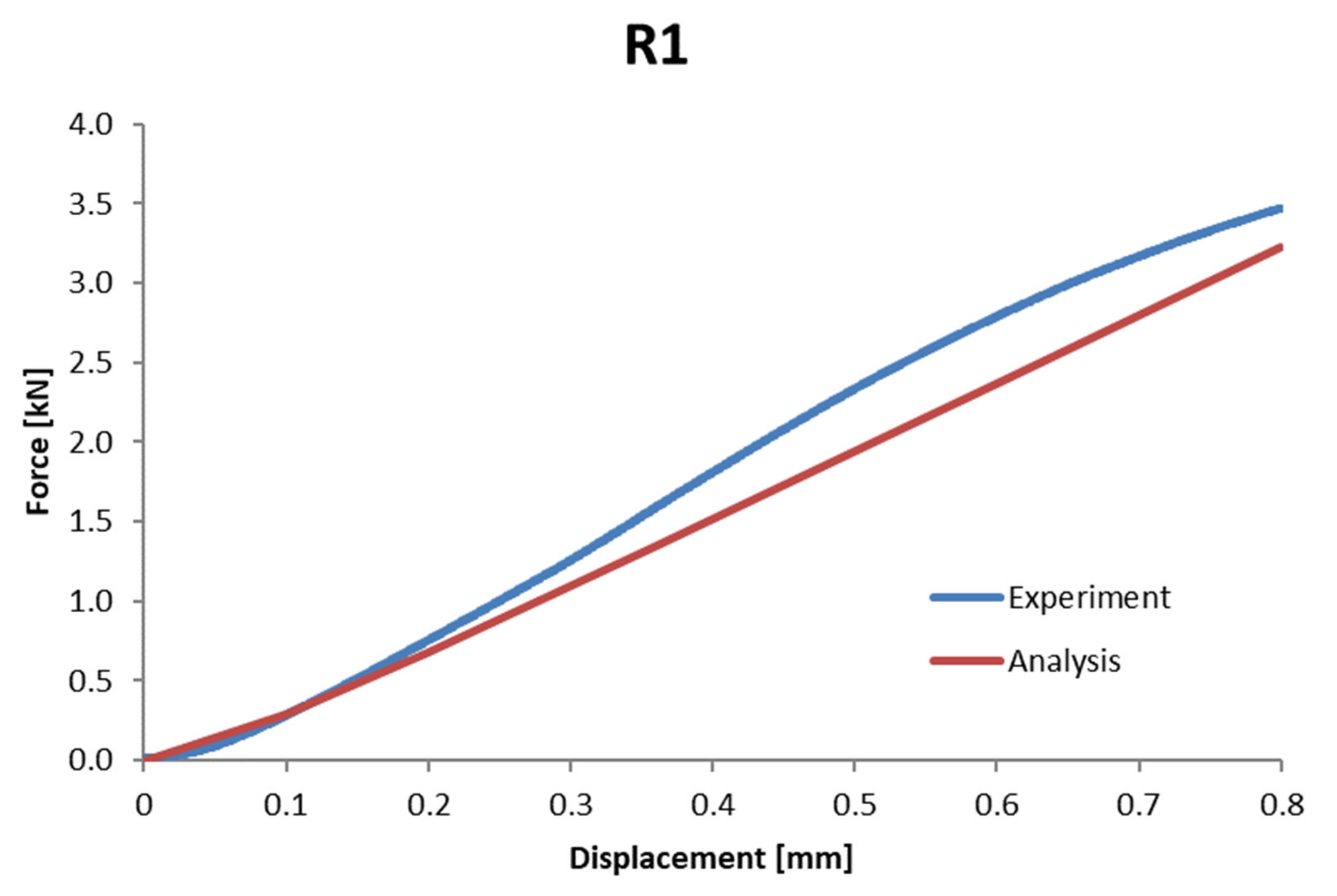
3.3. Method Validation—Step #2
4. Conclusions
Author Contributions
Funding
Institutional Review Board Statement
Informed Consent Statement
Data Availability Statement
Acknowledgments
Conflicts of Interest
References
- Robles-Linares, J.A.; Ramírez-Cedillo, E.; Siller, H.R.; Rodríguez, C.A.; Martínez-López, J.I. Parametric Modeling of Biomimetic Cortical Bone Microstructure for Additive Manufacturing. Materials 2019, 12, 913. [Google Scholar] [CrossRef] [PubMed] [Green Version]
- Huiskes, H.W. On the modelling of long bones in structural analyses. J. Biomech. 1982, 15, 65–69. [Google Scholar] [CrossRef] [Green Version]
- Mughal, U.N.; Khawaja, H.A.; Moatamedi, M. Finite element analysis of human femur bone. Int. J. Multiphysics 2015, 9, 101–108. [Google Scholar] [CrossRef]
- Arbag, H.; Korkmaz, H.H.; Ozturk, K.; Uyar, Y. Comparative Evaluation of Different Miniplates for Internal Fixation of Mandible Fractures Using Finite Element Analysis. J. Oral Maxillofac. Surg. 2008, 66, 1225–1232. [Google Scholar] [CrossRef]
- Martorelli, M.; Maietta, S.; Gloria, A.; de Santis, R.; Pei, E.; Lanzotti, A. Design and Analysis of 3D Customized Models of a Human Mandible. Procedia CIRP 2016, 49, 199–202. [Google Scholar] [CrossRef]
- Ilavarasi, P.U.; Anburajan, M. Design and finite element analysis of mandibular prosthesis. In Proceedings of the 3rd International Conference on Electronics Computer Technology, Kanyakumari, India, 8–10 April 2011; pp. 325–329. [Google Scholar] [CrossRef]
- Schuller-Götzburg, P.; Pleschberger, M.; Rammerstorfer, F.G.; Krenkel, C. 3D-FEM and histomorphology of mandibular reconstruction with the titanium functionally dynamic bridging plate. Int. J. Oral Maxillofac. Surg. 2009, 38, 1298–1305. [Google Scholar] [CrossRef]
- Chaudhry, A.; Sidhu, M.S.; Chaudhary, G.; Grover, S.; Chaudhry, N.; Kaushik, A. Evaluation of stress changes in the mandible with a fixed functional appliance: A finite element study. Am. J. Orthod. Dentofac. Orthop. 2015, 147, 226–234. [Google Scholar] [CrossRef]
- Dhanopia, A.; Bhargava, M. Finite Element Analysis of Human Fractured Femur Bone Implantation with PMMA Thermoplastic Prosthetic Plate. Procedia Eng. 2017, 173, 1658–1665. [Google Scholar] [CrossRef]
- Shreevats, R.; Cs, P.; Amarnath, B.C.; Shetty, A. An fem study on anterior tooth movement, in sliding mechanics with varying bracket slot and archwire dimension with and without alveolar bone loss. Int. J. Appl. Dent. Sci. 2018, 4, 197–202. [Google Scholar]
- Tajima, K.; Chen, K.K.; Takahashi, N.; Noda, N.; Nagamatsu, Y.; Kakigawa, H. Three-dimensional finite element modeling from CT images of tooth and its validation. Dent. Mater. J. 2009, 28, 219–226. [Google Scholar] [CrossRef] [Green Version]
- Borcic, J.; Braut, A. Finite Element Analysis in Dental Medicine. In Finite Element Analysis—New Trends and Developments; InTech: Rijeka, Croatia, 2012. [Google Scholar] [CrossRef] [Green Version]
- Benazzi, S.; Nguyen, H.N.; Kullmer, O.; Kupczik, K. Dynamic Modelling of Tooth Deformation Using Occlusal Kinematics and Finite Element Analysis. PLoS ONE 2016, 11, e0152663. [Google Scholar] [CrossRef]
- Opalach, K.; Porter-Sobieraj, J.; Zdroik, P. Stacking optimization of 3D printed continuous fiber layer designs. Adv. Eng. Softw. 2022, 164, 103077. [Google Scholar] [CrossRef]
- Kokot, G. Wyznaczanie Własności Mechanicznych Tkanek Kostnych z Zastosowaniem Cyfrowej Korelacji obrazu, Nanoindentacji oraz Symulacji Numerycznych; Wydawnictwo Politechniki Śląskiej: Gliwice, Poland, 2013. [Google Scholar]
- Zhang, G.; Xu, S.; Yang, J.; Guan, F.; Cao, L.; Mao, H. Combining specimen-specific finite-element models and optimization in cortical-bone material characterization improves prediction accuracy in three-point bending tests. J. Biomech. 2018, 76, 103–111. [Google Scholar] [CrossRef] [PubMed]
- Pruszyński, B. Radiologia. In Diagnostyka obrazowa Rtg, TK, USG, MR i Medycyna Nuklearna; Wydawnictwo Lekarskie PZWL: Warsaw, Poland, 2011. [Google Scholar]
- Barone, S.; Paoli, A.; Razionale, A.V. Creation of 3D Multi-Body Orthodontic Models by Using Independent Imaging Sensors. Sensors 2013, 13, 2033–2050. [Google Scholar] [CrossRef] [Green Version]
- Jamari, J.; Ammarullah, M.I.; Santoso, G.; Sugiharto, S.; Supriyono, T.; Prakoso, A.T.; Basri, H.; van der Heide, E. Computational Contact Pressure Prediction of CoCrMo, SS 316L and Ti6Al4V Femoral Head against UHMWPE Acetabular Cup under Gait Cycle. J. Funct. Biomater 2022, 13, 64. [Google Scholar] [CrossRef]
- Makowski, P.; Kus, W. Trabecular bone numerical homogenization with the use of buffer zone. Comput. Assist. Methods Eng. Sci. 2014, 21, 113–121. [Google Scholar]
- Makowski, P.; Kuś, W. Optimization of bone scaffold structures using experimental and numerical data. Acta Mech. 2016, 227, 139–149. [Google Scholar] [CrossRef]
- Ramezanzadehkoldeh, M.; Skallerud, B.H. MicroCT-based finite element models as a tool for virtual testing of cortical bone. Med. Eng. Phys. 2017, 46, 12–20. [Google Scholar] [CrossRef]
- Szucs, A.; Bujtar, P.; Sandor, G.; Barabas, J. Finite Element Analysis of the Human Mandible to Assess the Eect of Removing an Impacted Third Molar. J. Can. Dent. Assoc. 2010, 76, a72. [Google Scholar]
- Rokonuzzaman, M.; Sakai, T. Calibration of the parameters for a hardening–softening constitutive model using genetic algorithms. Comput. Geotech. 2010, 37, 573–579. [Google Scholar] [CrossRef]
- Bujtr, P.; Sndor GK, B.; Bojtos, A.; Szcs, A.; Barabs, J. Finite element analysis of the human mandible at 3 different stages of life. Oral Surg. Oral Med. Oral Pathol. Oral Radiol. Endodontology 2010, 110, 301–309. [Google Scholar] [CrossRef] [PubMed]
- Takahashi, V.; Lematre, M.; Fortineau, J.; Lethiecq, M. Elastic parameters characterization of multilayered structures by air-coupled ultrasonic transmission and genetic algorithm. Ultrasonics 2022, 119, 106619. [Google Scholar] [CrossRef] [PubMed]
- MazurkiewiczŁ, A.; Bukała, J.; Małachowski, J.; Tomaszewski, M.; Buszman, P.P. BVS stent optimisation based on a parametric model with a multistage validation process. Mater. Des. 2021, 198, 109363. [Google Scholar] [CrossRef]
- Mazurkiewicz, L.; Małachowski, J.; Damaziak, K.; Tomaszewski, M. Evaluation of the response of fibre reinforced composite repair of steel pipeline subjected to puncture from excavator tooth. Compos. Struct. 2018, 202, 1126–1135. [Google Scholar] [CrossRef]
- Raponi, E.; Fiumarella, D.; Boria, S.; Scattina, A.; Belingardi, G. Methodology for parameter identification on a thermoplastic composite crash absorber by the Sequential Response Surface Method and Efficient Global Optimization. Compos. Struct. 2021, 278, 114646. [Google Scholar] [CrossRef]
- Cappelli, L.; Balokas, G.; Montemurro, M.; Dau, F.; Guillaumat, L. Multi-scale identification of the elastic properties variability for composite materials through a hybrid optimisation strategy. Compos. Part B Eng. 2019, 176, 107193. [Google Scholar] [CrossRef]
- Guan, F.; Han, X.; Mao, H.; Wagner, C.; Yeni, Y.N.; Yang, K.H. Application of Optimization Methodology and Specimen-Specific Finite Element Models for Investigating Material Properties of Rat Skull. Ann. Biomed. Eng. 2011, 39, 85–95. [Google Scholar] [CrossRef]
- Qian, J.; Xu, W.; Mu, L.; Wu, A. Calibration of soil parameters based on intelligent algorithm using efficient sampling method. Undergr. Space 2021, 6, 329–341. [Google Scholar] [CrossRef]
- Wang, Y.; Zeng, X.; Sheng, Y.; Yang, X.; Wang, F. Multi-objective parameter identification and optimization for dislocation-dynamics-based constitutive modeling of Ti–6Al–4V alloy. J. Alloy. Compd. 2020, 821, 153460. [Google Scholar] [CrossRef]
- Yao, D.; Duan, Y.; Li, M.; Guan, Y. Hybrid identification method of coupled viscoplastic-damage constitutive parameters based on BP neural network and genetic algorithm. Eng. Fract. Mech. 2021, 257, 108027. [Google Scholar] [CrossRef]
- Rodrigues, A.F.F.; dos Santos, J.V.A.; Lopes, H. Identification of material properties of green laminate composite plates using bio-inspired optimization algorithms. Procedia Struct. Integr. 2022, 37, 684–691. [Google Scholar] [CrossRef]
- LSTC. LS-Dyna Keyword User’s Manual, Volume I-III, R11; Livemore Software Technology Corporation (LSTC): Livermore, CA, USA, 2018. [Google Scholar]
- Baranowski, P.; Gieleta, R.; Malachowski, J.; Damaziak, K.; Mazurkiewicz, L. Split Hopkinson Pressure Bar impulse experimental measurement with numerical validation. Metrol. Meas. Syst. 2014, 21, 47–58. [Google Scholar] [CrossRef] [Green Version]
- Baranowski, P.; Kucewicz, M.; Malachowski, J.; Sielicki, P.W. Failure behavior of a concrete slab perforated by a deformable bullet. Eng. Struct. 2021, 245, 112832. [Google Scholar] [CrossRef]
- Burkacki, M.; Wolański, W.; Suchoń, S.; Joszko, K.; Gzik-Zroska, B.; Sybilski, K.; Gzik, M. Finite element head model for the crew injury assessment in a light armoured vehicle. Acta Bioeng. Biomech. 2022, 22, 173–183. [Google Scholar] [CrossRef]
- Sybilski, K.; Mazurkiewicz, Ł.; Jurkojć, J.; Michnik, R. Małachowski, J. Evaluation of the effect of muscle forces implementation on the behavior of a dummy during a head-on collision. Acta Bioeng. Biomech. 2021, 23, 137–147. [Google Scholar] [CrossRef]


| Tissue | Young Modulus [GPa] | Poisson Ratio [-] | Density [kg/m3] |
|---|---|---|---|
| bone (compact) [3] | 20.0 | 0.37 | - |
| bone (compact) [4] | 15.0 | 0.30 | 2000.0 |
| bone (compact) [5] | 14.0 | 0.30 | - |
| porous tissue [6] | 2.0 | - | - |
| bone (compact) [7] | 20.0 | 0.30 | - |
| bone (compact) [8] | 10.5 | 0.30 | - |
| porous tissue [8] | 1.29 | 0.30 | - |
| bone (compact) [9] | 13.7 | 0.30 | - |
| porous tissue [9] | 7.93 | 0.30 | - |
| tooth [9] | 20.0 | 0.30 | - |
| bone (compact) [10] | 16.7 | 0.30 | 1750.0 |
| bone (compact) [11] | 20.0 | 0.30 | - |
| bone (compact) [12] | 13.8 | 0.30 | - |
| bone (compact) [13] | 13.7 | 0.38 | - |
| bone (compact) [14] | 13.7 | 0.30 | - |
| porous tissue [14] | 0.5 | 0.30 | - |
| Sample Number | Dimension A (Height) (mm) | Dimension B (Thickness) (mm) | L (Length) (mm) | Cross-Sectional Area P (mm2) | Moment of Inertia on the Bending Plane I (mm4) | Bending Strength Index W (mm3) | Distance between Supports Δ (mm) |
|---|---|---|---|---|---|---|---|
| F1 | 11.58 | 7.39 | 68.14 | 85.58 | 956.29 | 165.16 | 46 |
| F2 | 11.35 | 6.68 | 70.73 | 75.82 | 813.92 | 143.42 | 46 |
| F3 | 11.46 | 7.20 | 68.78 | 82.51 | 903.04 | 157.60 | 46 |
| R1 | 11.56 | 7.34 | 70.10 | 84.85 | 944.91 | 163.48 | 46 |
| L1 | 11.58 | 7.38 | 68.49 | 85.46 | 954.99 | 164.94 | 46 |
| B1 | 11.59 | 7.39 | 69.25 | 85.65 | 958.77 | 165.45 | 46 |
| B2 | 11.17 | 7.33 | 67.80 | 81.88 | 851.30 | 152.43 | 46 |
| Mean | 11.47 | 7.244 | 69.04 | 83.11 | 911.89 | 158.93 | 46 |
| Standard deviation | ±0.15 | ±0.24 | ±0.98 | ±3.30 | ±54.07 | ±7.71 | - |
| Manufacturer | Testing Machine | Test Load, Max. | Test Speed Range | Accuracy of the Test Speed | Position Transducer Travel Resolution |
|---|---|---|---|---|---|
| Zwick/Roell | Kappa 50 DS | 50.0 kN | 0.001 mm/h to 100.0 mm/min | <±0.1% | 0.068 nm |
| Resolution | Size of a Single Pixel | Distance between Scans | Field of View |
|---|---|---|---|
| 793 × 793 pixels | 0.15 mm | 0.15 mm | 118.95 × 118.95 mm |
| Values According to the Hounsfield Scale HU | Percentage of Individual Ranges According to the Hounsfield Scale | |||||
|---|---|---|---|---|---|---|
| L1 | F1 | F2 | F3 | B1 | R1 | |
| <600 | 8.96% | 11.22% | 13.06% | 9.95% | 8.16% | 14.15% |
| 600–800 | 3.84% | 2.94% | 6.17% | 1.38% | 1.89% | 2.07% |
| 800–1000 | 4.85% | 3.61% | 7.85% | 1.88% | 3.18% | 2.65% |
| 1000–1200 | 5.39% | 7.65% | 12.06% | 2.99% | 4.35% | 3.74% |
| 1200–1400 | 5.99% | 20.78% | 16.95% | 6.05% | 5.02% | 6.17% |
| 1400–1600 | 7.38% | 27.32% | 23.93% | 23.14% | 7.14% | 18.67% |
| 1600–1800 | 17.87% | 18.66% | 15.23% | 34.48% | 16.52% | 34.34% |
| 1800–2000 | 23.55% | 5.95% | 2.99% | 12.98% | 26.79% | 18.71% |
| 2000–2200 | 15.74% | 1.33% | 1.16% | 4.14% | 19.35% | 4.97% |
| 2200–2400 | 5.84% | 0.37% | 0.52% | 1.83% | 5.51% | 0.94% |
| >2400 | 0.57% | 0.18% | 0.08% | 1.20% | 2.09% | 0.36% |
| Coefficients | Value |
|---|---|
| a* | 0.388524 |
| b* | 4.419.3 |
| c* | 2.20939 |
| d* | 1.17823 |
| Sample | Stiffness Determined from the Experiment (N/mm2) | Stiffness Determined from Optimization (N/mm2) | Difference (%) |
|---|---|---|---|
| L1 | 5263.7 | 5259.9 | 0.072% |
| F1 | 4897.4 | 4905.1 | −0.157% |
| F2 | 4080.1 | 3901.9 | 4.368% |
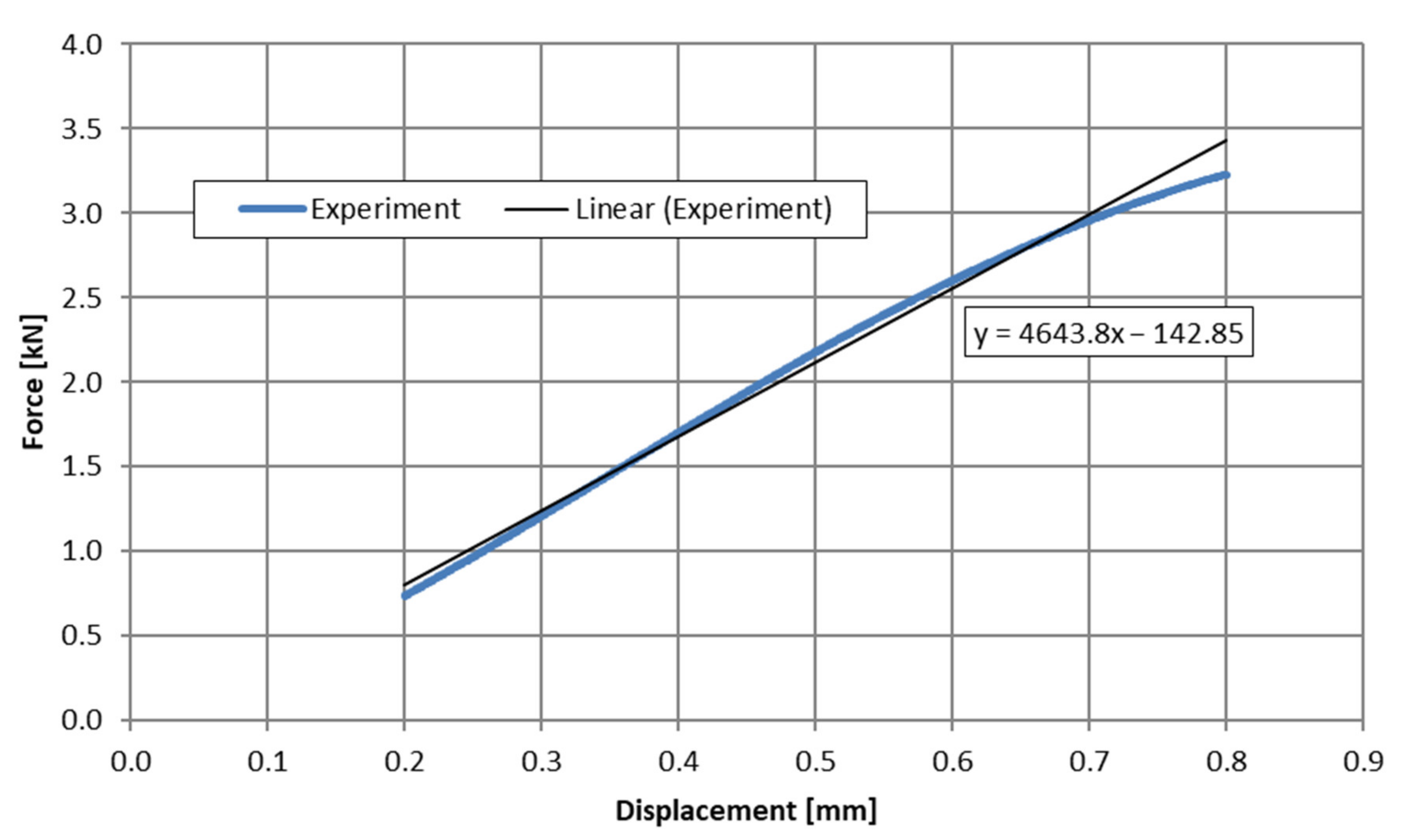
| F3 | 4643.8 | 4543.9 | 2.151% |
| B1 | 4569.3 | 4585.8 | −0.361% |
| Values According to the Hounsfield Scale HU | Middle Value | Bone Density ρ (kg/m3) | Young Modulus E (MPa) (Calculated) | Percentage of Particular Layer in the Total Sample (%) | L1 | F1 | F2 | F3 | B1 |
|---|---|---|---|---|---|---|---|---|---|
| Number of Voxels | |||||||||
| <600 | 500 | 5523.995 | 9969.031 | 10.27% | 19,923 | 24,831 | 25,767 | 20,777 | 16,743 |
| 600–800 | 700 | 5965.873 | 10,915.16 | 3.24% | 8533 | 6513 | 12,174 | 2880 | 3870 |
| 800–1000 | 900 | 6407.751 | 11,873.88 | 4.27% | 10,781 | 7992 | 15,478 | 3920 | 6524 |
| 1000–1200 | 1100 | 6849.629 | 12,844.46 | 6.49% | 11,991 | 16,921 | 23,785 | 6237 | 8931 |
| 1200–1400 | 1300 | 7291.507 | 13,826.27 | 10.96% | 13,319 | 45,989 | 33,445 | 12,629 | 10,301 |
| 1400–1600 | 1500 | 7733.385 | 14,818.75 | 17.78% | 16,406 | 60,468 | 47,211 | 48,317 | 14,645 |
| 1600–1800 | 1700 | 8175.263 | 15,821.39 | 20.55% | 39,732 | 41,309 | 30,040 | 72,013 | 33,888 |
| 1800–2000 | 1900 | 8617.141 | 16,833.75 | 14.45% | 52,351 | 13,160 | 5909 | 27,112 | 54,958 |
| 2000–2200 | 2100 | 9059.019 | 17,855.4 | 8.34% | 35,001 | 2933 | 2294 | 8643 | 39,687 |
| 2200–2400 | 2300 | 9500.897 | 18,885.98 | 2.81% | 12,989 | 812 | 1027 | 3816 | 11,302 |
| >2400 | 2500 | 9942.775 | 19,925.13 | 0.82% | 1274 | 397 | 166 | 2504 | 4279 |
| Mean | 7733.385 | 15,360.02 | 222,300 | 221,325 | 197,296 | 208,848 | 205,128 | ||
| Sample | Stiffness Determined from the Experiment (N/mm2) | Stiffness Determined from Optimization (N/mm2) | Difference (%) |
|---|---|---|---|
| R1 | 4682.2 | 4353.6 | 7.02% |
Publisher’s Note: MDPI stays neutral with regard to jurisdictional claims in published maps and institutional affiliations. |
© 2022 by the authors. Licensee MDPI, Basel, Switzerland. This article is an open access article distributed under the terms and conditions of the Creative Commons Attribution (CC BY) license (https://creativecommons.org/licenses/by/4.0/).
Share and Cite
Pietroń, K.; Mazurkiewicz, Ł.; Sybilski, K.; Małachowski, J. Correlation of Bone Material Model Using Voxel Mesh and Parametric Optimization. Materials 2022, 15, 5163. https://doi.org/10.3390/ma15155163
Pietroń K, Mazurkiewicz Ł, Sybilski K, Małachowski J. Correlation of Bone Material Model Using Voxel Mesh and Parametric Optimization. Materials. 2022; 15(15):5163. https://doi.org/10.3390/ma15155163
Chicago/Turabian StylePietroń, Kamil, Łukasz Mazurkiewicz, Kamil Sybilski, and Jerzy Małachowski. 2022. "Correlation of Bone Material Model Using Voxel Mesh and Parametric Optimization" Materials 15, no. 15: 5163. https://doi.org/10.3390/ma15155163
APA StylePietroń, K., Mazurkiewicz, Ł., Sybilski, K., & Małachowski, J. (2022). Correlation of Bone Material Model Using Voxel Mesh and Parametric Optimization. Materials, 15(15), 5163. https://doi.org/10.3390/ma15155163