
Experimental Investigation and Parametric Optimization of the Tungsten Inert Gas Welding Process Parameters of Dissimilar Metals

 ,
,  , , and
Abstract
:1. Introduction
2. Literature Review
2.1. Consideration during Welding Dissimilar Metals
2.2. Some Related Studies
3. Materials and Method
3.1. Base Materials
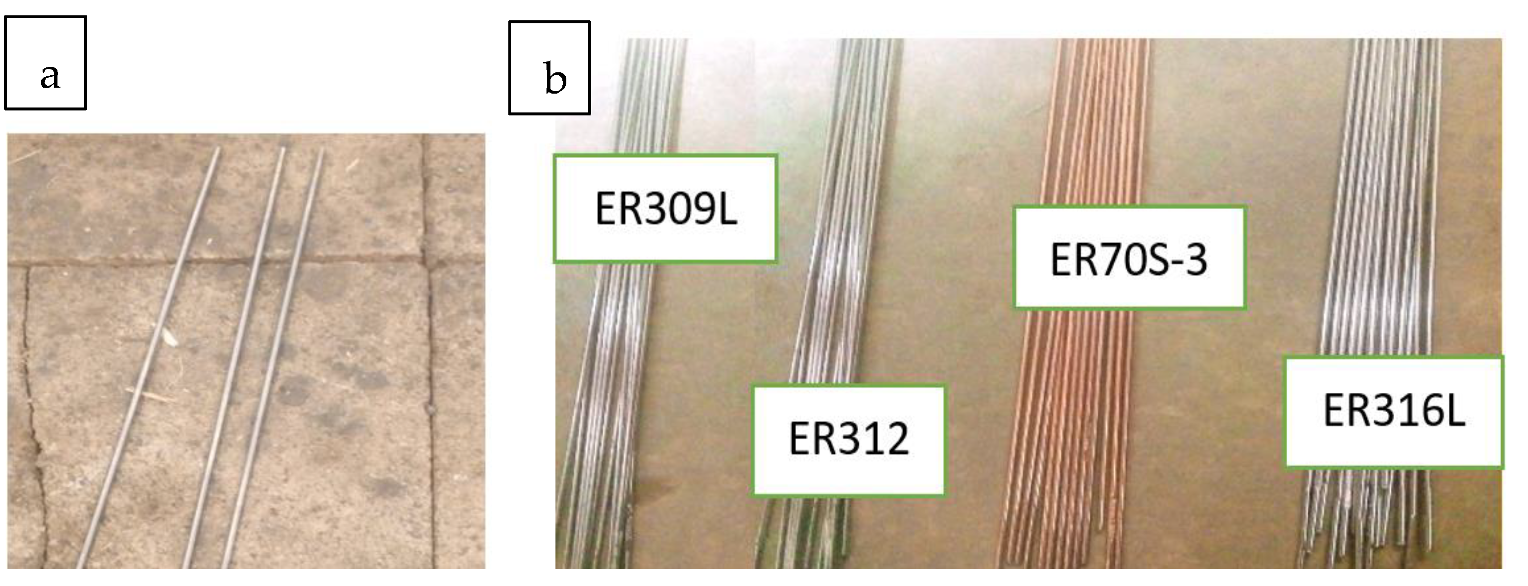
3.2. Material Used for Filler
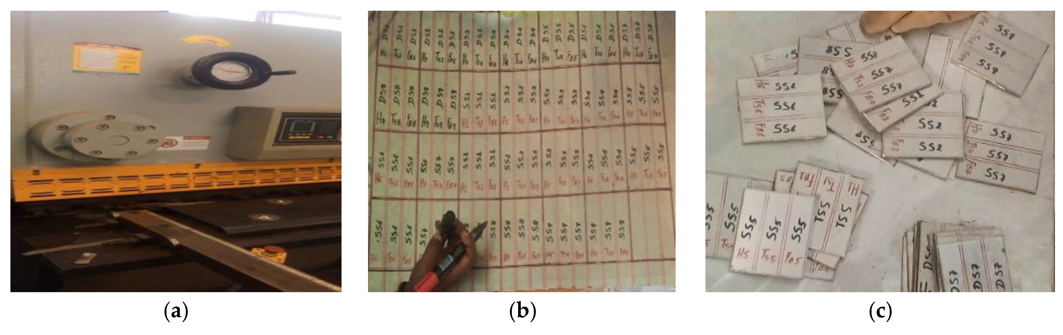
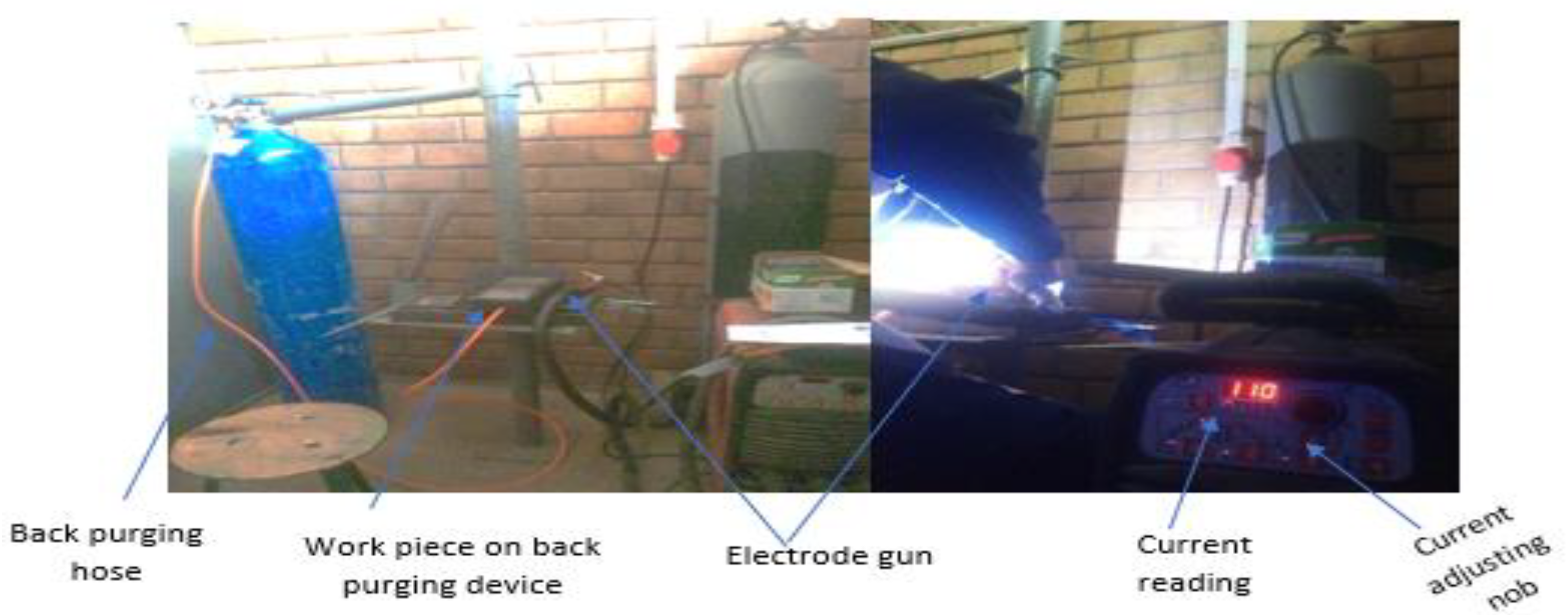
3.3. Experimental Set-up, Sample Preparation, and Welding Conditions
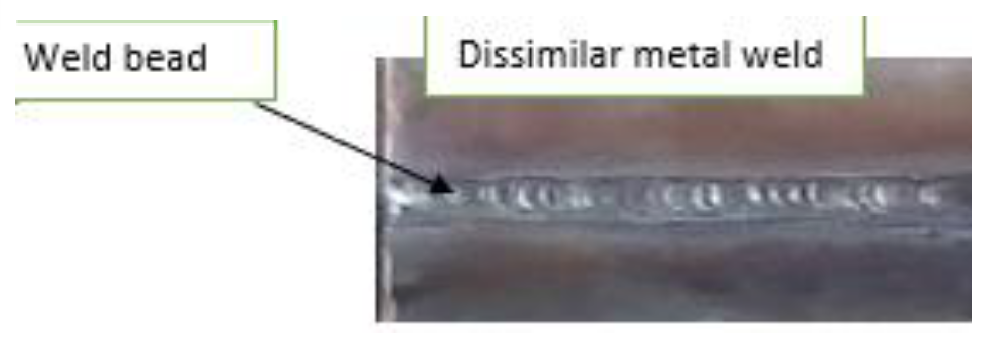
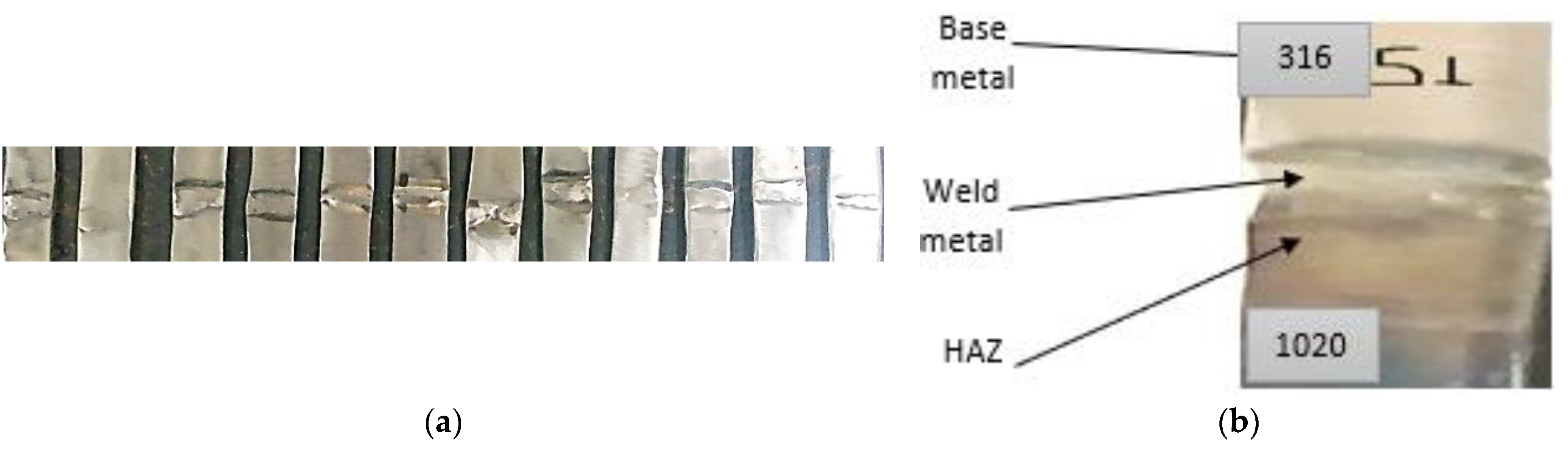
3.4. Weld Geometry and Defect Test
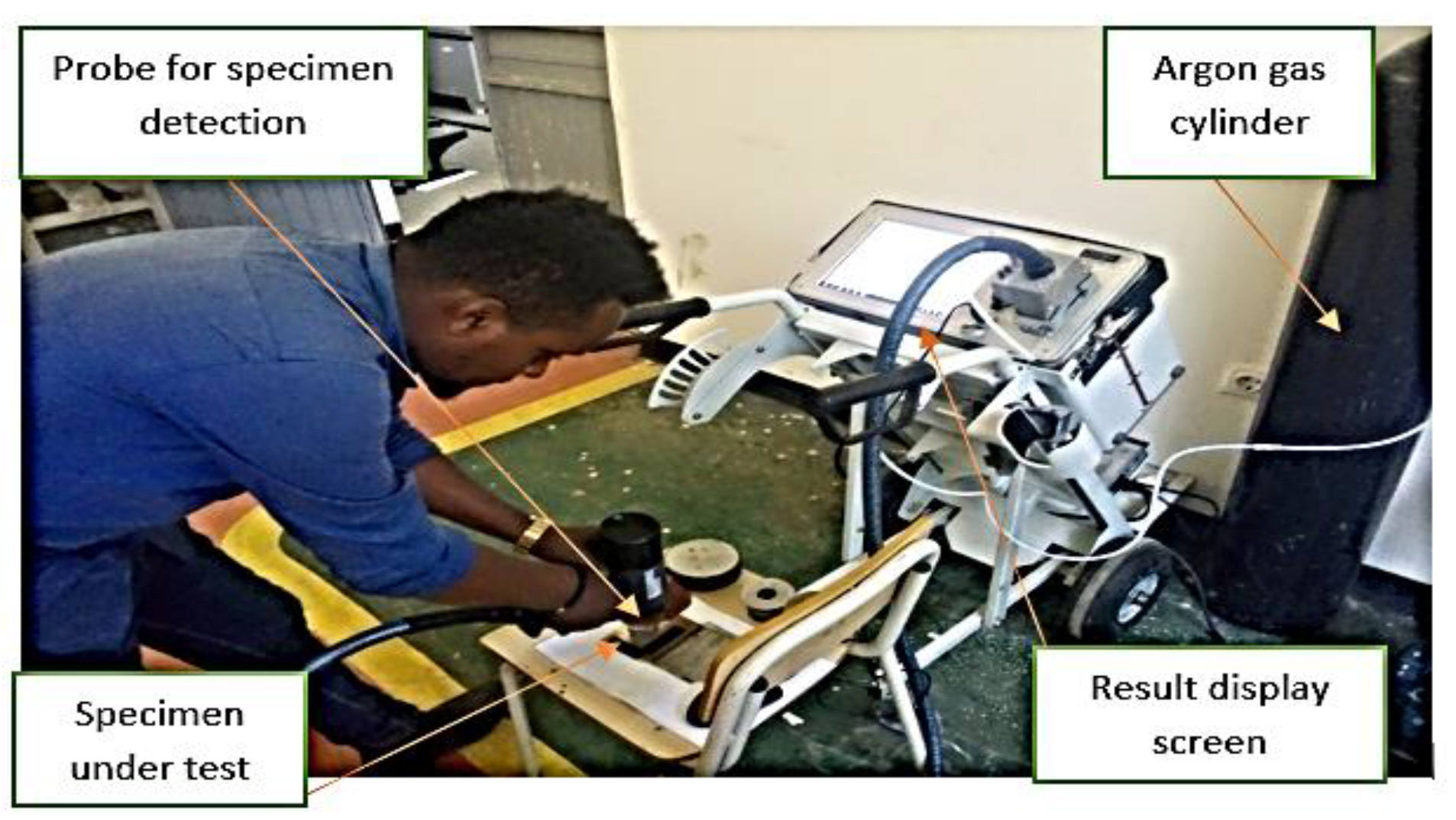
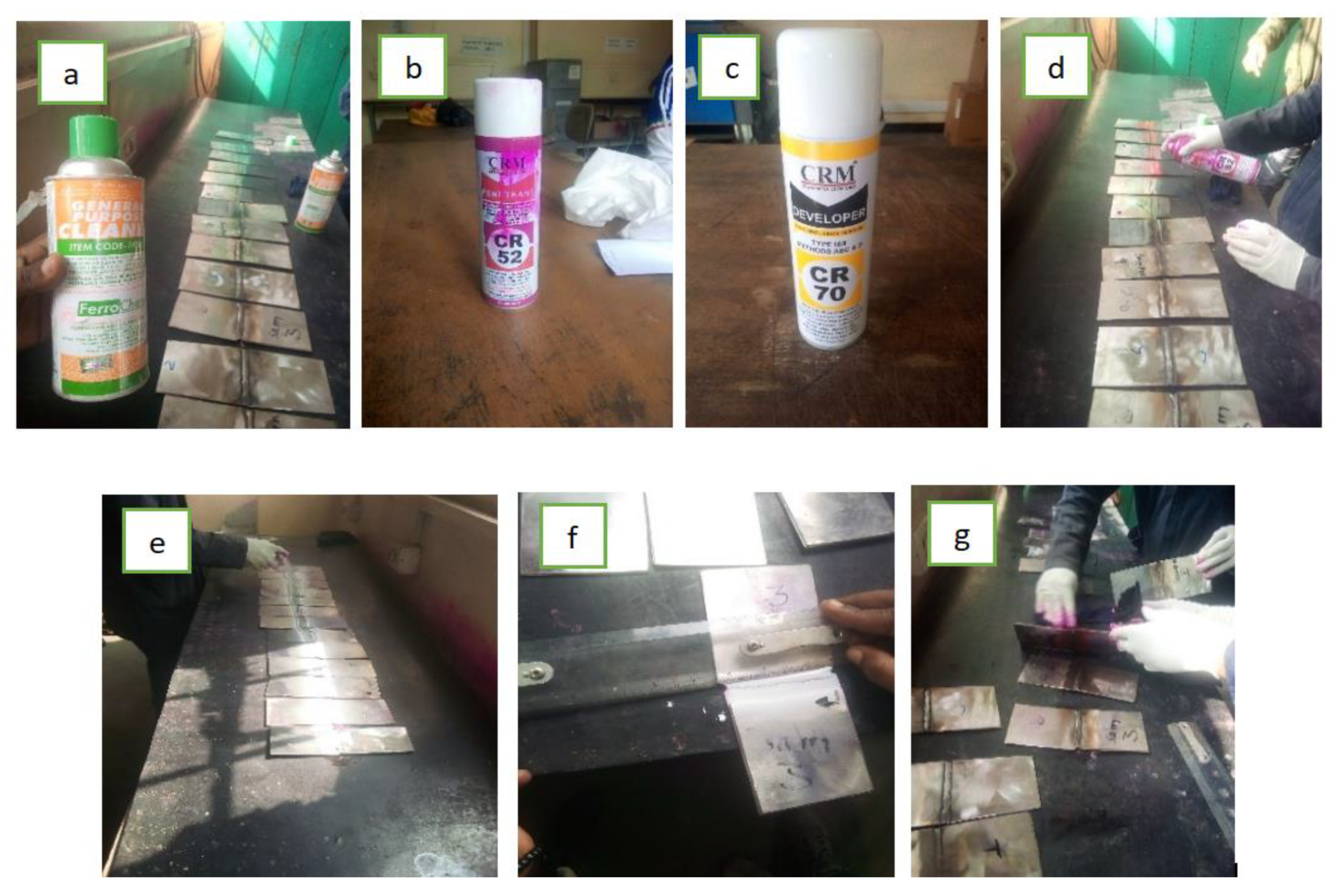
3.5. Liquid Penetrant Test (PT)
3.6. Mechanical Property Testing
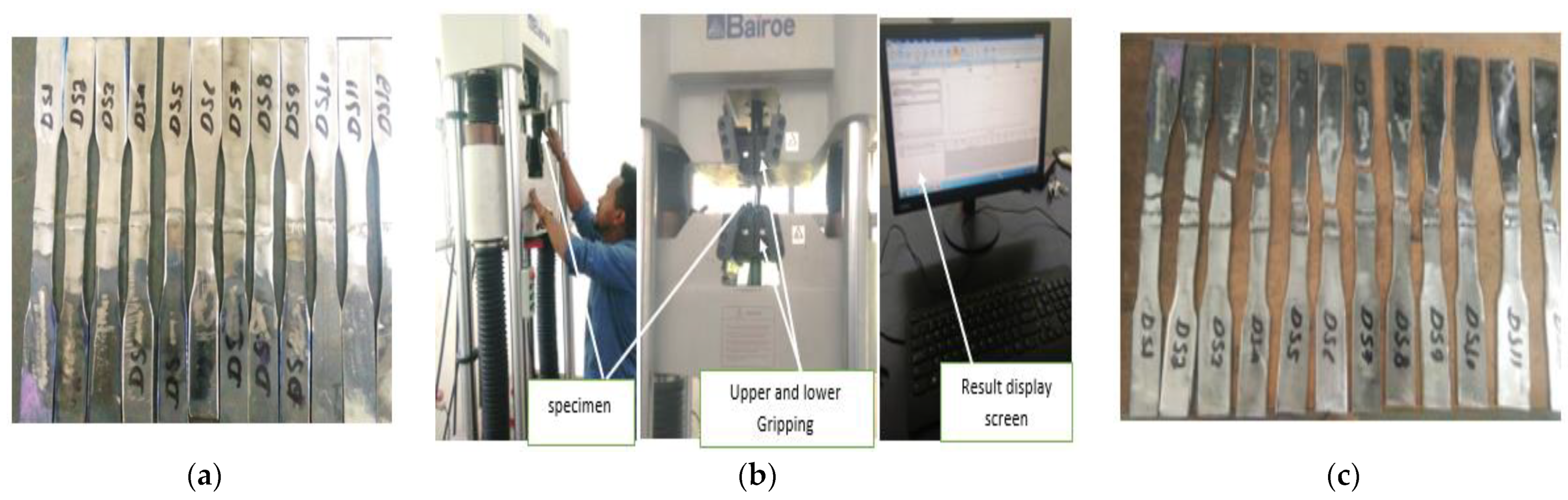
3.7. Tensile Strength
3.8. Hardness Testing
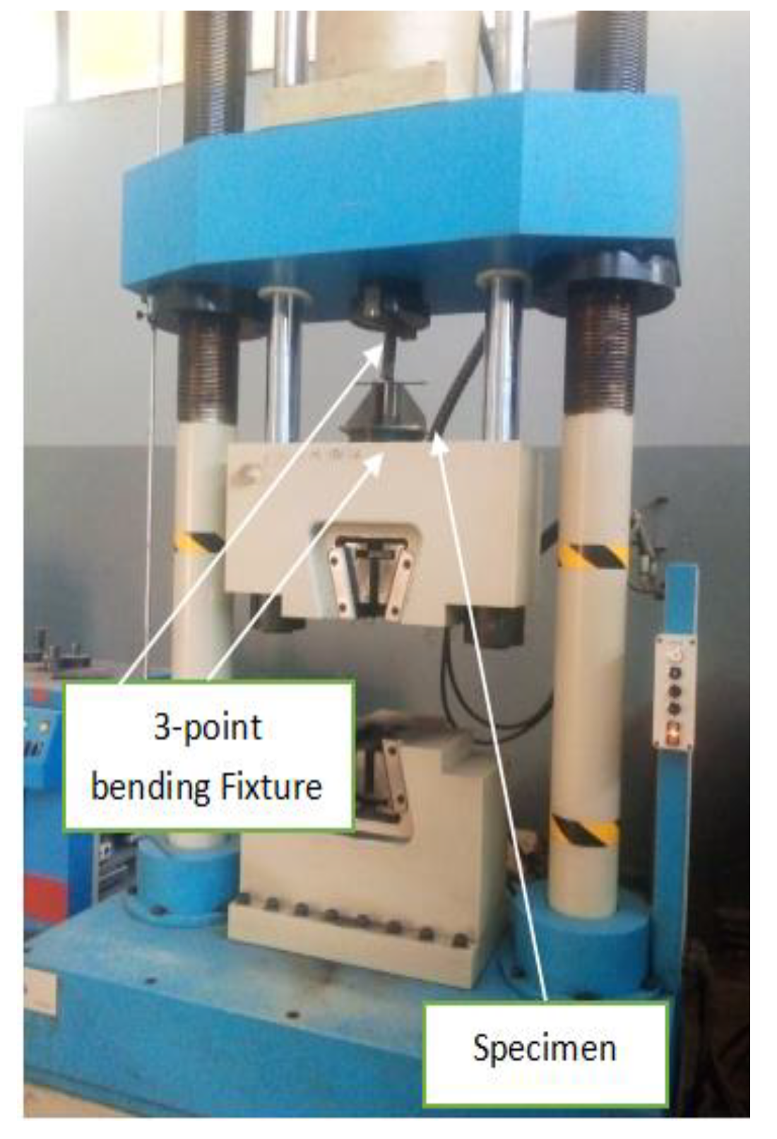
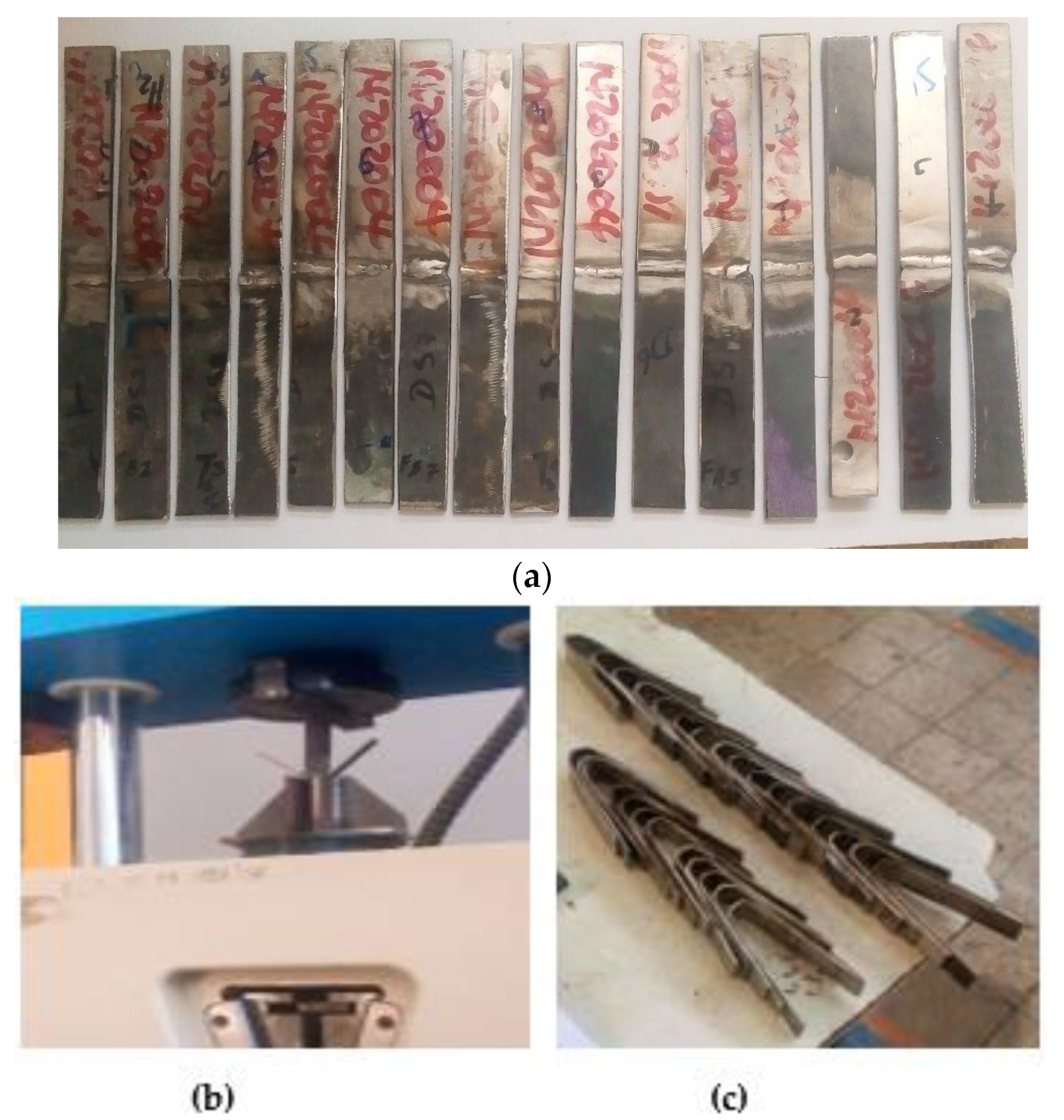
3.9. Flexural Testing
3.10. Microstructure and Microhardness Testing
3.11. Taguchi Method
3.12. ANOVA (Analysis of Variance)
4. Results and Discussion
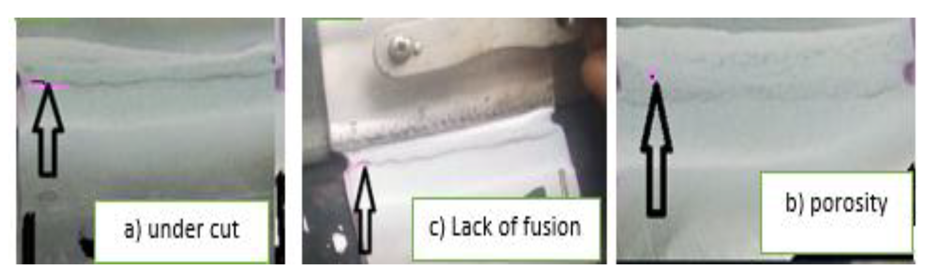
4.1. Liquid Penetrant and Visual Defect Testing
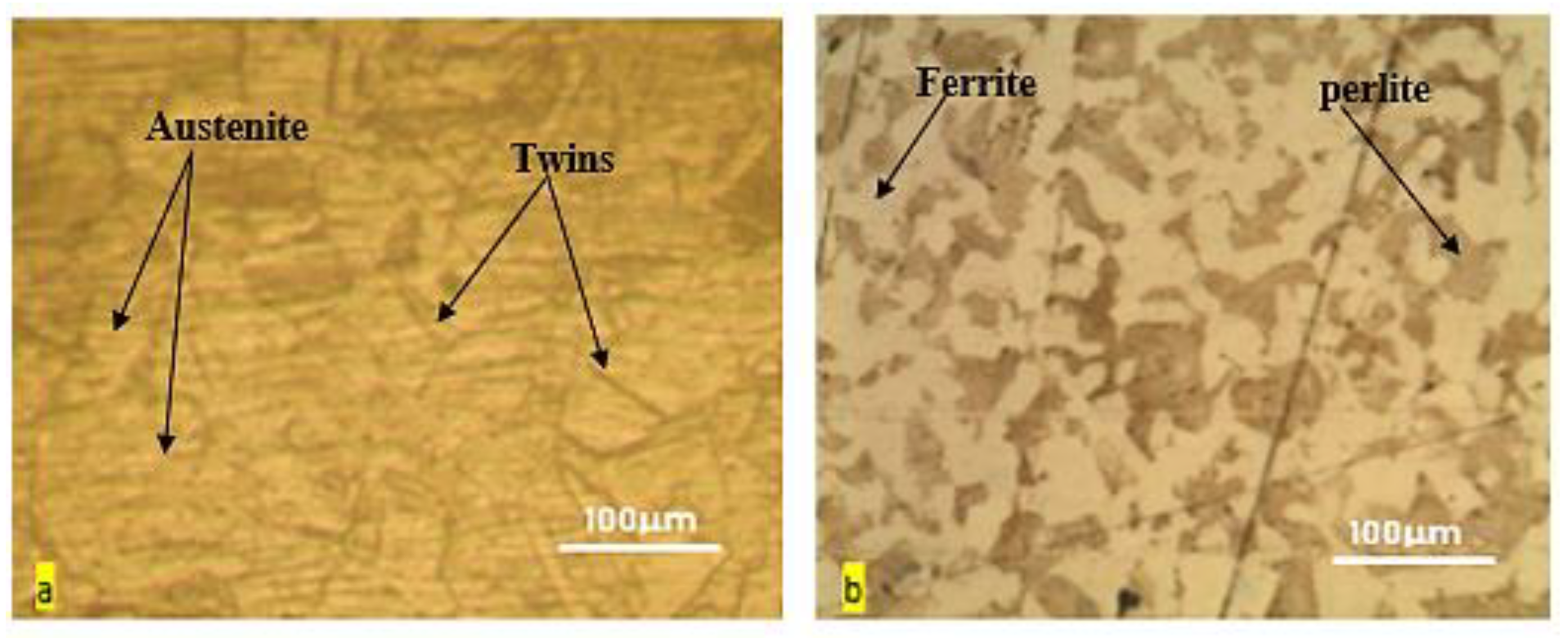
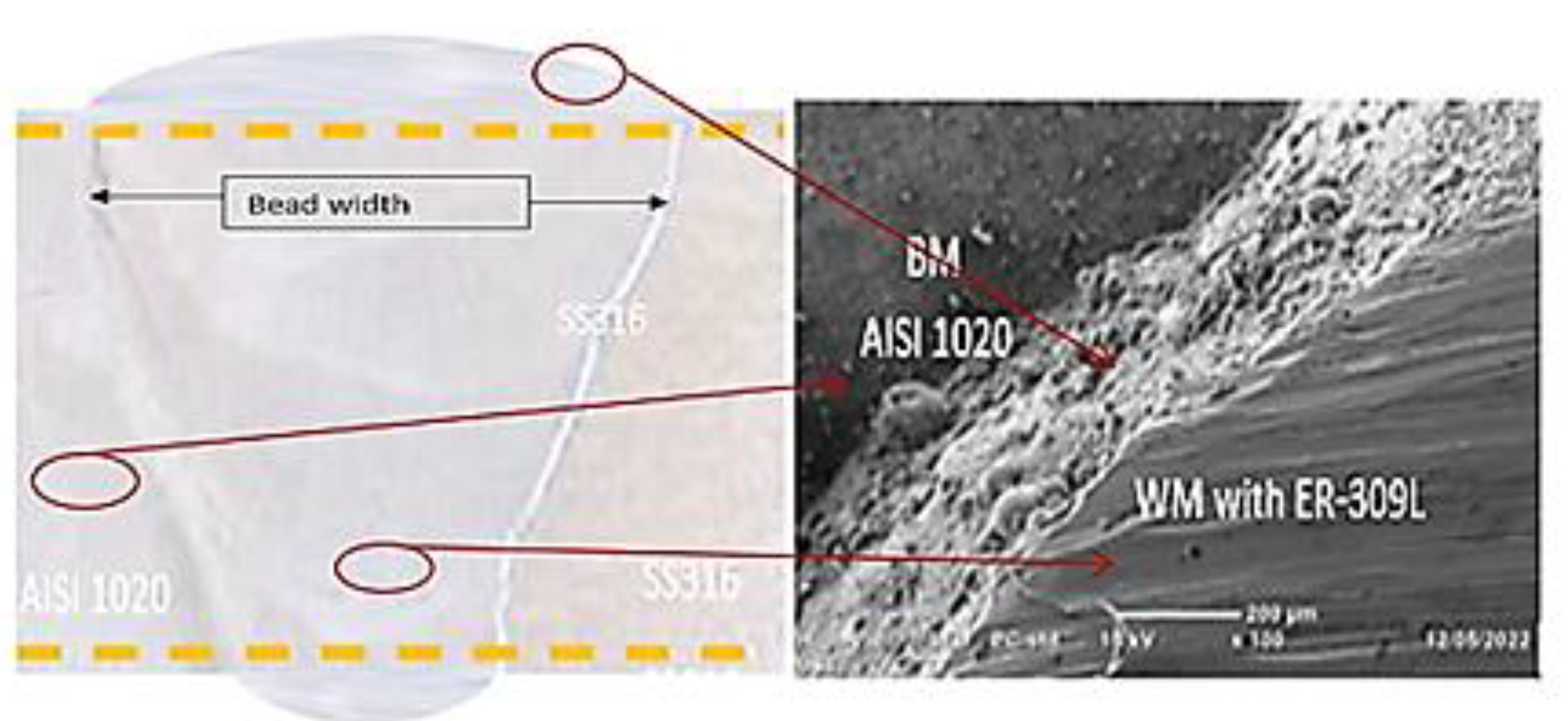
4.2. Microstructural Analysis of Welded Metals
4.3. Fractography Analysis
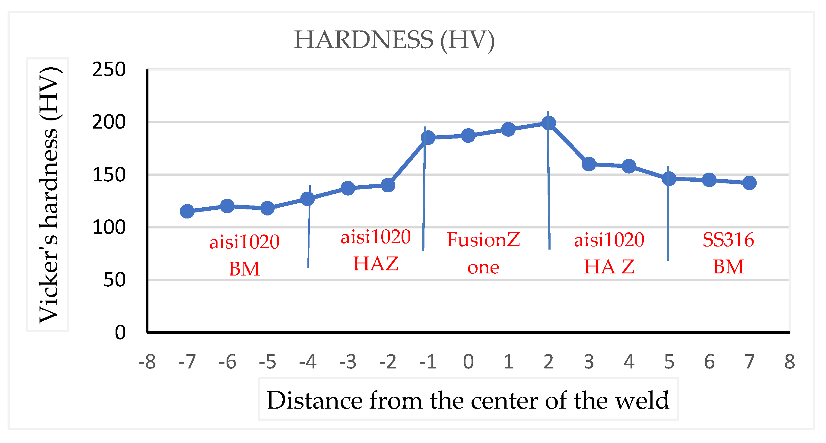
4.4. Microhardness Analysis
4.5. Mechanical Properties
4.6. Tensile Strength Result Analysis
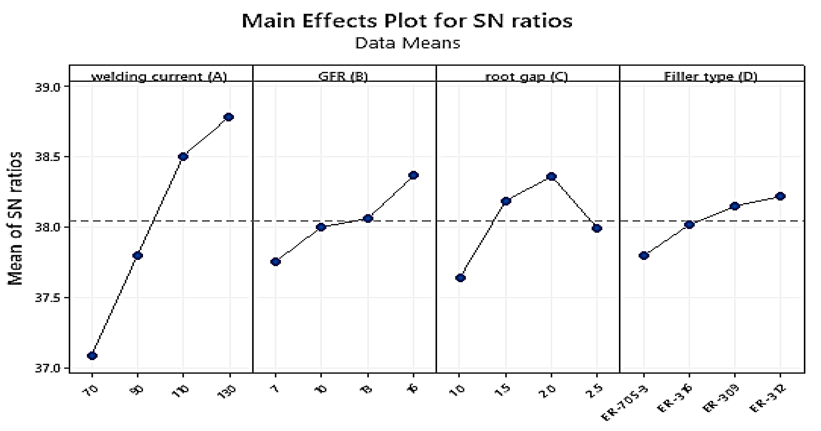
4.7. Hardness Test Results Analysis
4.8. Flexural Strength Result Analysis
4.9. Bead Width Result Analysis
4.10. Desirability Function Analysis (DFA)
4.11. Confirmation Test
5. Conclusions
Author Contributions
Funding
Acknowledgments
Conflicts of Interest
References
- Lee, C.-H.; Chang, K.-H. Prediction of residual stresses in welds of similar and dissimilar steel weldments. J. Mater Sci. 2007, 42, 6607–6613. [Google Scholar] [CrossRef]
- Sędek, P.; Brozda, J.; Wang, L.; Withers, P.J. Residual stress relief in MAG welded joints of dissimilar steels. Int. J. Press. Vessel. Pip. 2003, 80, 705–713. [Google Scholar] [CrossRef]
- Shushan, S.M.; Charles, E.A.; Congleton, J. The environment assisted cracking of diffusion bonded stainless to carbon steel joints in an aqueous chloride solution. Corros. Sci. 1996, 38, 673–686. [Google Scholar] [CrossRef]
- Khana, M.M.A.; Romoli, L.; Fiaschi, M.; Dini, G.; Sarri, F. Laser beam welding of dissimilar stainless steels in a fillet joint configuration. J. Mater. Process. Technol. 2012, 212, 856–867. [Google Scholar] [CrossRef]
- Wang, S.; Ma, Q.; Li, Y. Characterization of microstructure, mechanical properties and corrosion resistance of dissimilar welded joint between 2205 duplex stainless steel and 16MnR. Mater Des. 2011, 32, 831–837. [Google Scholar] [CrossRef]
- Jeyaprakash, N.; Haile, A.; Arunprasath, M. The Parameters and Equipments Used in TIG Welding: A Review. Int. J. Eng. Sci. 2015, 4, 11–20. Available online: www.theijes.com (accessed on 15 April 2022).
- Kumar, S.; Singh, P.; Patel, D.; Prasad, S.B. Optimization of TIG welding process parameters using Taguchi’s analysis and response surface methodology. Int. J. Mech. Eng. Technol. 2017, 8, 932–941. [Google Scholar]
- Karunakaran, N.; Balasubramanian, V. Effect of pulsed current on temperature distribution, weld bead profiles and characteristics of gas tungsten arc welded aluminum alloy joints. Trans. Nonferrous Met. Soc. China 2011, 21, 278–286. [Google Scholar] [CrossRef]
- Chaudhari, R.; Loharkar, P.K.; Ingle, A. Applications and challenges of arc welding methods in dissimilar metal joining. IOP Conf. Ser. Mater Sci. Eng. 2020, 810, 012006. [Google Scholar] [CrossRef]
- Kah, P.; Jukka Martikainen, M.S. Trends in joining dissimilar metals by welding. Appl. Mech. Mater. 2013, 440, 269–276. [Google Scholar] [CrossRef]
- Dak, G.; Pandey, C. Experimental investigation on microstructure, mechanical properties, and residual stresses of dissimilar welded joint of martensitic P 92 and AISI 304 L austenitic stainless steel. Int. J. Press. Vessel. Pip. 2021, 194, 104536. [Google Scholar] [CrossRef]
- Khan, M.; Dewan, M.W.; Sarkar, M.Z. Effects of welding technique, filler metal and post-weld heat treatment on stainless steel and mild steel dissimilar welding joint. J. Manuf. Processes 2021, 64, 1307–1321. [Google Scholar] [CrossRef]
- Ramakrishnan, A.; Rameshkumar, T.; Rajamurugan, G.; Sundarraju, G.; Selvamuthukumaran, D. Experimental investigation on mechanical properties of TIG welded dissimilar AISI 304 and AISI 316 stainless steel using 308 filler rod. Mater. Today Proc. 2021, 45, 8207–8211. [Google Scholar] [CrossRef]
- Satputaley, S.S.; Waware, Y.; Ksheersagar, K.; Jichkar, Y.; Khonde, K. Experimental investigation on effect of TIG welding process on chromoly 4130 and aluminum 7075-T6. Mater. Today Proc. 2021, 41, 991–994. [Google Scholar] [CrossRef]
- Ramadan, N.; Boghdadi, A. Parametric Optimization of TIG Welding Influence on Tensile Strength of Dissimilar Metals SS-304 and Low Carbon Steel by Using Taguchi Approach. Am. J. Eng. Res. 2020, 9, 7–14. [Google Scholar]
- Vennimalai Rajan, A.; Mathalai Sundaram, D.C.; Vembathurajesh, A.; Nagaraja, R.; Chakravarthy Samy Durai, J.; Nagaraja, R. Analysis and Experimental investigation of Weld Characteristics for TIG Welding in Dissimilar Metals. Int. J. Emerg. Trends Eng. Res. 2020, 1, 278–287. [Google Scholar] [CrossRef]
- Anbarasu, P.; Yokeswaran, R.; Godwin Antony, A.; Sivachandran, S. Investigation of filler material influence on hardness of TIG welded joints. Mater. Today Proc. 2020, 21, 964–967. [Google Scholar] [CrossRef]
- Kausar, A. Study of Weld Quality characteristics of Tungsten Inert Gas Welding of Dissimilar Metals SS 316L and IS 2062 Plates. Int. J. Res. Appl. Sci. Eng. Technol. 2019, 7, 759–767. [Google Scholar] [CrossRef]
- Hazari, H.R.; Balubai, M.; Suresh Kumar, D.; Haq, A.U. Experimental investigation of TIG welding on AA 6082 and AA 8011. In Materials Today: Proceedings; Elsevier: Amsterdam, The Netherlands, 2019; pp. 818–822. [Google Scholar]
- Sayed, A.R.; Kumbhare, Y.V.; Ingole, N.G.; Dhengale, P.T.; Dhanorkar, N.R. A Review Study of Dissimilar Metal Welds of Stainless Steel and Mild Steel by TIG Welding Process. Int. J. Res. Appl. Sci. Eng. Technol. 2019, 7, 370–373. [Google Scholar] [CrossRef]
- Kumar, A.; Sharma, V.; Baruaole, N.S. Experimental Investigation of TIG welding of Stainless Steel 202 and Stainless Steel 410 using Taguchi Technique. Mody Univ. Int. J. Comput. Eng. Res. 2017, 1, 96–99. Available online: https://ijcer.in/ojs/index.php/IJCER/article/view/18 (accessed on 10 February 2022).
- Devakumar, D.; Jabaraj, D.B.; Bupesh Raja, V.K.; Jayaprakash, J. Experimental Investigation of DSS/HRS GTAW Weldments. Indian J. Sci. Technol. 2016, 9, 1–6. [Google Scholar] [CrossRef]
- Kumar, L.S.; Verma, S.M.; Prasad, P.R.; Kumar, P.K.; Shanker, T.S. Experimental investigation for welding aspects of AISI 304 & 316 by Taguchi technique for the process of TIG & MIG welding. Int. J. Eng. Trends Technol. 2011, 2, 28–33. [Google Scholar]
- Efunda. Definition of Low-Carbon Steels. 2012. Available online: http://www.efunda.com/materials/alloys/carbon_steels/low_carbon.cfm (accessed on 16 March 2022).
- Inweld.com. Data Sheet for 316L Stainless Steel: 94621. Available online: https://inweldcorporation.com/downloads/316LDataSheet.pdf (accessed on 11 January 2022).
- Unibraze Corporation. Er70S-3 Carbon Steel Welding Wire. 2000, pp. 1–2. Available online: http://www.unibraze.com/DataSheets/Data70S-3.pdf (accessed on 5 January 2022).
- Esme, U.; Bayramoglu, M.; Kazancoglu, Y.; Ozgun, S. Optimization of weld bead geometry in TIG welding process using grey relation analysis and Taguchi method. Mater. Tehnol. 2009, 43, 143–149. [Google Scholar]
- Davis, J.R. Tensile Testing; ASM international: Almere, The Netherlands, 2004. [Google Scholar]
- AWS Committee. Welding Inspection Handbook, 3rd ed.; AWS Committee: Doral, FL, USA, 2000. [Google Scholar]
- Johnson, L. How to Calculate Flexural Strength|Sciencing. 2022. Available online: https://sciencing.com/calculate-flexural-strength-5179141.html (accessed on 2 January 2022).
- Dmitri, K. Flexural strength tests of ceramics. 2021. Available online: https://www.substech.com/dokuwiki/doku.php?id=flexural_strength_tests_of_ceramics (accessed on 1 April 2022).
- ASM Handbook Committee. Mechanical Testing and Evaluation; ASM Handbook Committee: Materials Park, OH, USA, 2000; Volume 8, pp. 143–151. [Google Scholar]
- Callister, W.D. An Introduction: Material Science and Engineering; John Wiley Sons Inc.: Hoboken, NJ, USA, 2007. [Google Scholar]
- Krishnaiah, K.; Shahabudeen, P. Applied Design of Experiments and Taguchi Methods; PHI Learning Pvt. Ltd.: Delhi, India, 2012. [Google Scholar]
- Ross, P.J. Taguchi Techniques for Quality Engineering: Loss Function, Orthogonal Experiments, Parameter and Tolerance Design; Mcgraw-Hill: New York, NY, USA, 1996. [Google Scholar]
- Karna, S.K.; Sahai, R. An overview on Taguchi method. Int. J. Eng. Math Sci. 2012, 1, 1–7. [Google Scholar]
- Raissi, S.; Farsani, R.-E. Statistical Process Optimization Through Multi-Response Surface Methodology. World Acad. Sci. Eng. Technol. 2009, 3, 247–251. [Google Scholar]
- Harrington, E.C. The desirability function. Ind. Qual. Control. 1965, 21, 494–498. [Google Scholar]
- Derringer, G.; Suich, R. Simultaneous optimization of several response variables. J. Qual. Technol. 1980, 12, 214–219. [Google Scholar] [CrossRef]
- Moi, S.C.; Pal, P.K.; Bandyopadhyay, A. Design optimization of TIG welding process for AISI 316 L stainless steel. Int. J. Recent Technol. Eng. 2019, 8, 5348–5354. [Google Scholar]
- Hedhibi, A.C.; Touileb, K.; Djoudjou, R.; Ouis, A.; Alrobei, H.; Ahmed, M.M.Z. Mechanical properties and microstructure of TIG and ATIG welded 316 L austenitic stainless steel with multi-components flux optimization using mixing design method and particle swarm optimization (PSO). Materials 2021, 14, 7139. [Google Scholar] [CrossRef]
- Moslemi, N.; Redzuan, N.; Ahmad, N.; Hor, T.N. Effect of current on characteristic for 316 stainless steel welded joint including microstructure and mechanical properties. Procedia CIRP 2015, 26, 560–564. [Google Scholar] [CrossRef] [Green Version]
- Pasupathy, J.; Ravisankar, V. Parametric Optimization of TIG Welding Parameters using Taguchi Method for Dissimilar Joint. Int. J. Sci. Eng. Res. 2013, 4, 25–28. [Google Scholar]
- Wahule, A.; Wasankar, K. Multi-response optimization of process parameters of TIG welding for dissimilar metals (SS-304 and Fe-410) using grey relational analysis. Int. Res. J. Eng. Technol. 2018, 5, 986–993. [Google Scholar]
- Patil, S.R.; Waghmare, C.A. Optimization of MIG welding parameters for improving strength of welded joints. Int. J. Adv. Eng. Res. Stud. 2013, 14, 16. [Google Scholar]


| Materials (AISI Designation) | Chemical Composition (wt.%) | ||||||||||
|---|---|---|---|---|---|---|---|---|---|---|---|
| C | Mn | P | S | Si | Cr | Ni | Mo | N | Fe | ||
| Base metals | AISI 316 | 0.08 | 1.95 | 0.045 | 0.03 | 0.70 | 16.50 | 12.06 | 2.40 | 0.10 | 65.180 |
| AISI1020 | 0.20 | 0.40 | 0.042 | 0.03 | - | - | - | - | - | 99.328 | |
| Weld metal | Filler used | ||||||||||
| ER-316 | 0.063 | 1.70 | 0.043 | 0.03 | 0.40 | 14.61 | 10.74 | 1.90 | 0.078 | - | |
| ER-309 | 0.063 | 1.75 | 0.041 | 0.03 | 0.67 | 17.99 | 9.81 | 0.89 | 0.015 | 0.52 | |
| ER-312 | 0.119 | 1.72 | 0.034 | 0.03 | 0.46 | 20.25 | 11.05 | 0.89 | 0.015 | 0.52 | |
| ER-70S-3 | 0.112 | 1.03 | 0.027 | 0.03 | 0.42 | 2.843 | 1.89 | 0.36 | 0.015 | 0.25 | |
| Materials (AWS Designation) | Chemical Composition (wt.%) | |||||||||||
|---|---|---|---|---|---|---|---|---|---|---|---|---|
| C | Mn | P | S | Si | Cr | Ni | Mo | N | Cu | Fe | ||
| Filler metals | ER-316L | 0.03 | 1.92 | 0.043 | 0.03 | 0.42 | 16.98 | 12.05 | 2.21 | 0.09 | - | Bal. |
| ER-309L | 0.03 | 2.00 | 0.04 | 0.03 | 0.80 | 23.06 | 13.20 | 0.75 | - | 0.74 | Bal. | |
| ER-312 | 0.11 | 1.95 | 0.03 | 0.03 | 0.50 | 25.00 | 10.00 | 0.75 | - | 0.74 | Bal. | |
| ER-70S-3 | 0.10 | 0.98 | 0.021 | 0.03 | 0.46 | 0.14 | 0.12 | - | - | 0.35 | Bal. | |
| S. No | Process Parameter | Units | Levels | |||
|---|---|---|---|---|---|---|
| 1 | 2 | 3 | 4 | |||
| 1 | Welding current | Amp (A) | 70 | 90 | 110 | 130 |
| 2 | Root Gap | Mm | 1 | 1.5 | 2 | 2.5 |
| 3 | Gas flow rate | L/Min | 7 | 10 | 13 | 16 |
| 4 | Type of filler metals | Type | ER316 | ER309 | ER70S-3 | ER312 |
| S. No | Welding Current (A) | Gas Flow Rate (L/min) | Root Gap (mm) | Filler Type |
|---|---|---|---|---|
| S1 | 70 | 7 | 1 | ER70S-3 |
| S2 | 70 | 10 | 1.5 | ER316 |
| S3 | 70 | 13 | 2 | ER309 |
| S4 | 70 | 16 | 2.5 | ER312 |
| S5 | 90 | 7 | 1.5 | ER309 |
| S6 | 90 | 10 | 1 | ER312 |
| S7 | 90 | 13 | 2.5 | ER70S-3 |
| S8 | 90 | 16 | 2 | ER316 |
| S9 | 110 | 7 | 2 | ER312 |
| S10 | 110 | 10 | 2.5 | ER309 |
| S11 | 110 | 13 | 1 | ER316 |
| S12 | 110 | 16 | 1.5 | ER70S-3 |
| S13 | 130 | 7 | 2.5 | ER316 |
| S14 | 130 | 10 | 2 | ER70S-3 |
| S15 | 130 | 13 | 1.5 | ER312 |
| S16 | 130 | 16 | 1 | ER309 |
| Sample No | Non-Destructive Test Result |
|---|---|
| Sample 1 | Undercut |
| Sample 2 | Lack of fusion |
| Sample 3 | Defect-free |
| Sample 4 | Defect-free |
| Sample 5 | Lack of fusion |
| Sample 6 | Defect-free |
| Sample 7 | Defect-free |
| Sample 8 | Defect-free |
| Sample 9 | Defect-free |
| Sample 10 | Defect-free |
| Sample 11 | Defect-free |
| Sample 12 | Defect-free |
| Sample 13 | Porosity |
| Sample 14 | Defect-free |
| Sample 15 | Defect-free |
| Sample 16 | Defect-free |
| S. No | Process Parameter | Units | Levels | |||
|---|---|---|---|---|---|---|
| 1 | 2 | 3 | 4 | |||
| 1 | Welding current (A) | Amp (A) | 70 | 90 | 110 | 130 |
| 2 | Gas flow rate (B) | L/Min | 7 | 10 | 13 | 16 |
| 3 | Root gap (C) | mm | 1 | 1.5 | 2 | 2.5 |
| 4 | Type of filler metals (D) | Grade | ER-70S-3 | ER-316 | ER-309 | ER-312 |
| Sample No | Welding Current (A) | Gas Flow Rate (B) | Root Gap (C) | Filler Type (D) | Tensile Strength (MPa) | Signal-to-Noise Ratio |
|---|---|---|---|---|---|---|
| 1 | 70 | 7 | 1.0 | ER70S-3 | 390 | 51.8213 |
| 2 | 70 | 10 | 1.5 | ER316 | 420 | 52.4650 |
| 3 | 70 | 13 | 2.0 | ER309 | 460 | 53.2552 |
| 4 | 70 | 16 | 2.5 | ER312 | 442 | 52.9084 |
| 5 | 90 | 7 | 1.5 | ER309 | 450 | 53.0643 |
| 6 | 90 | 10 | 1.0 | ER312 | 410 | 52.2557 |
| 7 | 90 | 13 | 2.5 | ER70S-3 | 478 | 53.5886 |
| 8 | 90 | 16 | 2.0 | ER316 | 445 | 52.9672 |
| 9 | 110 | 7 | 2.0 | ER312 | 410 | 52.2557 |
| 10 | 110 | 10 | 2.5 | ER309 | 502 | 54.0141 |
| 11 | 110 | 13 | 1.0 | ER316 | 483 | 53.6789 |
| 12 | 110 | 16 | 1.5 | ER70S-3 | 486 | 53.7327 |
| 13 | 130 | 7 | 2.5 | ER316 | 398 | 51.9977 |
| 14 | 130 | 10 | 2.0 | ER70S-3 | 395 | 51.9319 |
| 15 | 130 | 13 | 1.5 | ER312 | 412 | 52.2979 |
| 16 | 130 | 16 | 1.0 | ER309 | 435 | 52.7698 |
| Level | Welding Current (A) | Gas Flow Rate (B) | Root Gap (C) | Filler Type (D) |
|---|---|---|---|---|
| 1 | 428.0 | 412.0 | 429.5 | 437.3 |
| 2 | 445.8 | 431.8 | 442.0 | 436.5 |
| 3 | 470.3 | 458.3 | 427.5 | 461.8 |
| 4 | 410.0 | 452.0 | 455.0 | 418.5 |
| Delta | 60.3 | 46.3 | 27.5 | 43.3 |
| Rank | 1 | 2 | 4 | 3 |
| Level | Welding Current (A) | Gas Flow Rate (B) | Root Gap (C) | Filler Type (D) |
|---|---|---|---|---|
| 1 | 52.61 | 52.28 | 52.63 | 52.77 |
| 2 | 52.97 | 52.67 | 52.89 | 52.78 |
| 3 | 53.42 | 53.21 | 52.60 | 53.28 |
| 4 | 52.25 | 53.09 | 53.13 | 52.43 |
| Delta | 1.17 | 0.92 | 0.52 | 0.85 |
| Rank | 1 | 2 | 4 | 3 |
| Source | DF | Seq SS | % Cont. | Adj SS | Adj MS | F | P |
|---|---|---|---|---|---|---|---|
| Welding current (A) | 3 | 3.00449 | 40.80 | 3.00449 | 1.00150 | 73.76 | 0.003 |
| Gas flow rate (B) | 3 | 2.13415 | 29.00 | 2.13415 | 0.71138 | 52.39 | 0.004 |
| Root gap (C) | 3 | 0.72768 | 9.90 | 0.72768 | 0.24256 | 17.86 | 0.020 |
| Filler type (D) | 3 | 1.45828 | 19.80 | 1.45828 | 0.48609 | 35.80 | 0.008 |
| Residual error | 3 | 0.04073 | 0.50 | 0.04073 | 0.01358 | ||
| Total | 15 | 7.36534 | 100.00 |
| Sample No | Welding Current (A) | Gas Flow Rate (B) | Root Gap (C) | Filler Type (D) | Hardness (HRB) | Signal-to-Noise Ratio |
|---|---|---|---|---|---|---|
| 1 | 70 | 7 | 1.0 | ER70S-3 | 64 | 36.1236 |
| 2 | 70 | 10 | 1.5 | ER316 | 72 | 37.1466 |
| 3 | 70 | 13 | 2.0 | ER309 | 75 | 37.5012 |
| 4 | 70 | 16 | 2.5 | ER312 | 76 | 37.6163 |
| 5 | 90 | 7 | 1.5 | ER309 | 78 | 37.8419 |
| 6 | 90 | 10 | 1.0 | ER312 | 75 | 37.5012 |
| 7 | 90 | 13 | 2.5 | ER70S-3 | 75 | 37.5012 |
| 8 | 90 | 16 | 2.0 | ER316 | 83 | 38.3816 |
| 9 | 110 | 7 | 2.0 | ER312 | 86 | 38.6900 |
| 10 | 110 | 10 | 2.5 | ER309 | 84 | 38.4856 |
| 11 | 110 | 13 | 1.0 | ER316 | 81 | 38.1697 |
| 12 | 110 | 16 | 1.5 | ER70S-3 | 86 | 38.6900 |
| 13 | 130 | 7 | 2.5 | ER316 | 83 | 38.3816 |
| 14 | 130 | 10 | 2.0 | ER70S-3 | 88 | 38.8897 |
| 15 | 130 | 13 | 1.5 | ER312 | 90 | 39.0849 |
| 16 | 130 | 16 | 1.0 | ER309 | 87 | 38.7904 |
| Level | Welding Current (A) | Gas Flow Rate (B) | Root Gap (C) | Filler Type (D) |
|---|---|---|---|---|
| 1 | 71.75 | 77.75 | 76.75 | 78.25 |
| 2 | 77.75 | 79.75 | 81.50 | 79.75 |
| 3 | 84.25 | 80.25 | 83.00 | 81.00 |
| 4 | 87.00 | 83.00 | 79.50 | 81.75 |
| Delta | 15.25 | 5.25 | 6.25 | 3.50 |
| Rank | 1 | 3 | 2 | 4 |
| Level | Welding Current (A) | Gas Flow Rate (B) | Root Gap (C) | Filler Type (D) |
|---|---|---|---|---|
| 1 | 37.24 | 38.43 | 38.42 | 37.71 |
| 2 | 38.54 | 38.32 | 37.89 | 39.02 |
| 3 | 38.57 | 38.10 | 38.54 | 38.35 |
| 4 | 38.74 | 38.24 | 38.24 | 38.01 |
| Delta | 1.50 | 0.34 | 0.65 | 1.30 |
| Rank | 1 | 4 | 3 | 2 |
| Source | DF | Seq SS | % Cont. | Adj SS | Adj MS | F | P |
|---|---|---|---|---|---|---|---|
| Welding current (A) | 3 | 6.88294 | 74.57 | 6.88294 | 2.29431 | 200.49 | 0.001 |
| GFR (B) | 3 | 0.75520 | 8.52 | 0.75520 | 0.25173 | 22.00 | 0.015 |
| Root gap (C) | 3 | 1.14149 | 12.37 | 1.14149 | 0.38050 | 33.25 | 0.008 |
| Filler type (D) | 3 | 0.41515 | 4.50 | 0.41515 | 0.13838 | 12.09 | 0.035 |
| Residual error | 3 | 0.03433 | 0.04 | 0.03433 | 0.01144 | ||
| Total | 15 | 9.22910 | 100 |
| Sample No | Welding Current (A) | Gas Flow Rate (B) | Root Gap (C) | Filler Type (D) | Flexural Strength (MPa) | Signal-to-Noise Ratio |
|---|---|---|---|---|---|---|
| 1 | 70 | 7 | 1.0 | ER703 | 555 | 54.8859 |
| 2 | 70 | 10 | 1.5 | ER316 | 605 | 55.6351 |
| 3 | 70 | 13 | 2.0 | ER309 | 670 | 56.5215 |
| 4 | 70 | 16 | 2.5 | ER312 | 640 | 56.1236 |
| 5 | 90 | 7 | 1.5 | ER309 | 692 | 56.8021 |
| 6 | 90 | 10 | 1.0 | ER312 | 655 | 56.3248 |
| 7 | 90 | 13 | 2.5 | ER703 | 620 | 55.8478 |
| 8 | 90 | 16 | 2.0 | ER316 | 679 | 56.6374 |
| 9 | 110 | 7 | 2.0 | ER312 | 545 | 54.7279 |
| 10 | 110 | 10 | 2.5 | ER309 | 662 | 56.4172 |
| 11 | 110 | 13 | 1.0 | ER316 | 505 | 54.0658 |
| 12 | 110 | 16 | 1.5 | ER703 | 440 | 52.8691 |
| 13 | 130 | 7 | 2.5 | ER316 | 588 | 55.3875 |
| 14 | 130 | 10 | 2.0 | ER703 | 525 | 54.4032 |
| 15 | 130 | 13 | 1.5 | ER312 | 480 | 53.6248 |
| 16 | 130 | 16 | 1.0 | ER309 | 595 | 55.4903 |
| Level | Welding Current (A) | Gas Flow Rate (B) | Root Gap (C) | Filler Type (D) |
|---|---|---|---|---|
| 1 | 617.5 | 595.0 | 577.5 | 535.0 |
| 2 | 661.5 | 611.8 | 554.3 | 594.3 |
| 3 | 538.0 | 568.8 | 604.8 | 654.8 |
| 4 | 547.0 | 588.5 | 627.5 | 580.0 |
| Delta | 123.5 | 43.0 | 73.3 | 119.8 |
| Rank | 1 | 4 | 3 | 2 |
| Level | Welding Current (A) | Gas Flow Rate (B) | Root Gap (C) | Filler Type (D) |
|---|---|---|---|---|
| 1 | 55.85 | 55.45 | 55.09 | 54.42 |
| 2 | 56.36 | 55.30 | 54.99 | 55.47 |
| 3 | 54.37 | 55.31 | 55.61 | 56.28 |
| 4 | 54.73 | 55.23 | 55.61 | 55.13 |
| Delta | 1.99 | 0.22 | 0.62 | 1.86 |
| Rank | 1 | 4 | 3 | 2 |
| Source | DF | Seq SS | % Cont. | Adj SS | Adj MS | F | P |
|---|---|---|---|---|---|---|---|
| Welding current (A) | 3 | 9.5245 | 46.57 | 9.52446 | 3.17482 | 190.89 | 0.001 |
| GFR (B) | 3 | 0.9838 | 4.8 | 0.98376 | 0.32792 | 19.72 | 0.018 |
| Root gap (C) | 3 | 3.2319 | 15.80 | 3.23193 | 1.07731 | 64.77 | 0.003 |
| Filler type (D) | 3 | 6.6638 | 32.58 | 6.66380 | 2.22127 | 133.55 | 0.001 |
| Residual error | 3 | 0.0499 | 0.25 | 0.04990 | 0.01663 | ||
| Total | 15 | 20.4538 | 100 |
| Sample No | Welding Current (A) | Gas Flow Rate (B) | Root Gap (C) | Filler Type (D) | Bead Width (mm) | Signal-to-Noise Ratio |
|---|---|---|---|---|---|---|
| 1 | 70 | 7 | 1.0 | ER703 | 7.50 | −17.5012 |
| 2 | 70 | 10 | 1.5 | ER316 | 7.05 | −16.9638 |
| 3 | 70 | 13 | 2.0 | ER309 | 6.90 | −16.7770 |
| 4 | 70 | 16 | 2.5 | ER312 | 6.90 | −16.7770 |
| 5 | 90 | 7 | 1.5 | ER309 | 7.00 | −16.9020 |
| 6 | 90 | 10 | 1.0 | ER312 | 7.80 | −17.8419 |
| 7 | 90 | 13 | 2.5 | ER703 | 6.80 | −16.6502 |
| 8 | 90 | 16 | 2.0 | ER316 | 6.21 | −15.8618 |
| 9 | 110 | 7 | 2.0 | ER312 | 7.70 | −17.7298 |
| 10 | 110 | 10 | 2.5 | ER309 | 7.50 | −17.5012 |
| 11 | 110 | 13 | 1.0 | ER316 | 8.00 | −18.0618 |
| 12 | 110 | 16 | 1.5 | ER703 | 7.10 | −17.0252 |
| 13 | 130 | 7 | 2.5 | ER316 | 7.45 | −17.4431 |
| 14 | 130 | 10 | 2.0 | ER703 | 7.80 | −17.8419 |
| 15 | 130 | 13 | 1.5 | ER312 | 7.90 | −17.9525 |
| 16 | 130 | 16 | 1.0 | ER309 | 8.00 | −18.0618 |
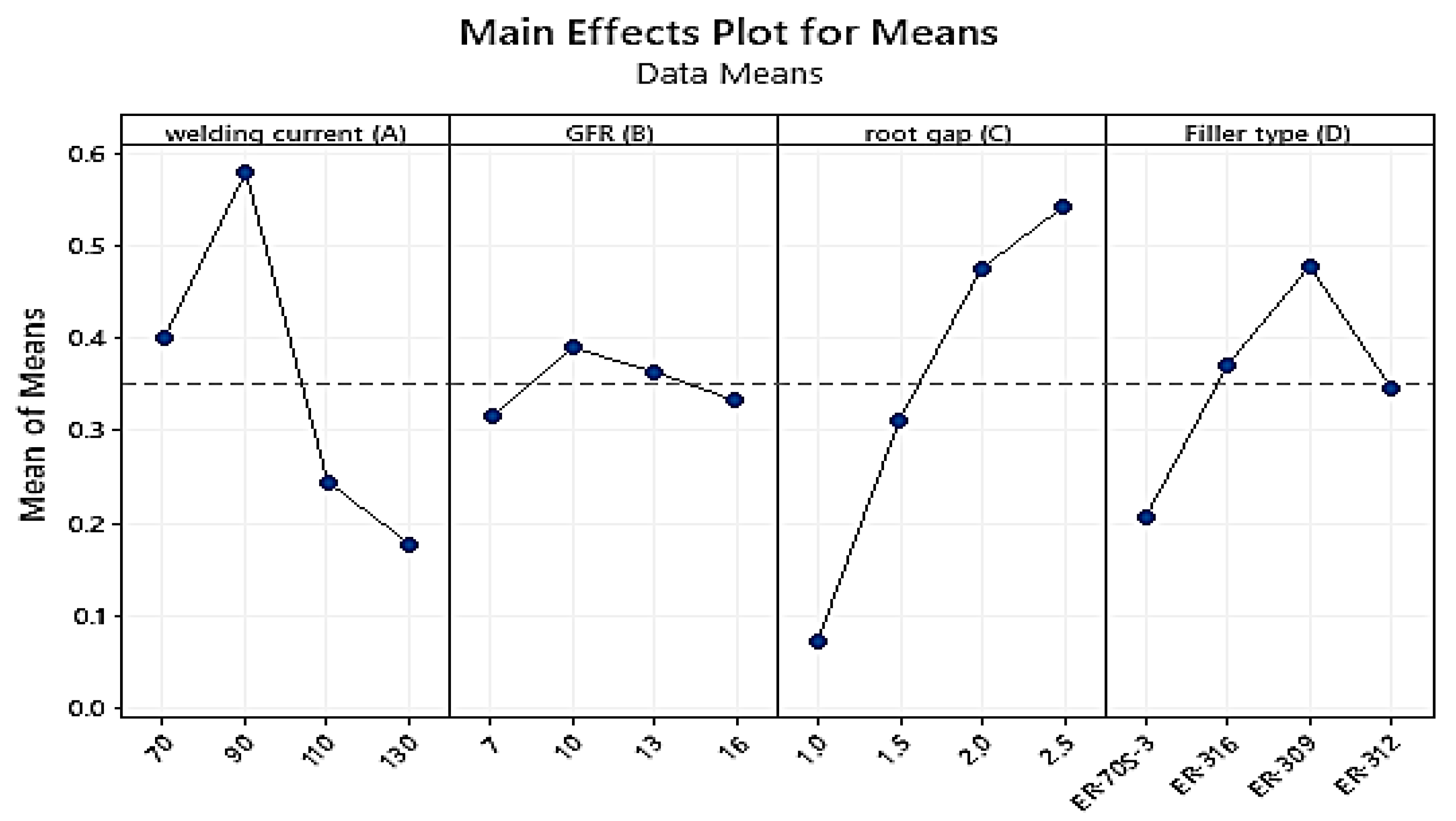
| Level | Welding Current (A) | Gas Flow Rate (B) | Root Gap (C) | Filler Type (D) |
|---|---|---|---|---|
| 1 | 7.088 | 7.412 | 7.825 | 7.300 |
| 2 | 6.953 | 7.538 | 7.262 | 7.177 |
| 3 | 7.575 | 7.400 | 7.152 | 7.350 |
| 4 | 7.787 | 7.053 | 7.162 | 7.575 |
| Delta | 0.835 | 0.485 | 0.673 | 0.397 |
| Rank | 1 | 3 | 2 | 4 |
| Level | Welding Current (A) | Gas Flow Rate (B) | Root Gap (C) | Filler Type (D) |
|---|---|---|---|---|
| 1 | −17.00 | −17.39 | −17.87 | −17.25 |
| 2 | −16.81 | −17.54 | −17.21 | −17.08 |
| 3 | −17.58 | −17.36 | −17.05 | −17.31 |
| 4 | −17.82 | −16.93 | −17.09 | −17.58 |
| Delta | 1.01 | 0.61 | 0.81 | 0.49 |
| Rank | 1 | 3 | 2 | 4 |
| Source | DF | Seq SS | % Cont. | Adj SS | Adj MS | F | P |
|---|---|---|---|---|---|---|---|
| Welding current (A) | 3 | 2.70740 | 46.35 | 2.70740 | 0.90247 | 31.29 | 0.009 |
| GFR (B) | 3 | 0.81780 | 14.00 | 0.81780 | 0.27260 | 9.45 | 0.049 |
| Root gap (C) | 3 | 1.73212 | 29.64 | 1.73212 | 0.57737 | 20.02 | 0.017 |
| Filler type (D) | 3 | 0.50032 | 8.56 | 0.50032 | 0.16677 | 5.78 | 0.092 |
| Residual error | 3 | 0.08652 | 1.45 | 0.08652 | 0.02884 | ||
| Total | 15 | 5.84416 | 100 |
| Sample No | Welding Current (A) | Gas Flow Rate (B) | Root Gap (C) | Filler Type (D) | Tensile Strength (MPa) | Hardness (HRB) | Flexural Strength (MPa) | Bead Width (mm) |
|---|---|---|---|---|---|---|---|---|
| 1 | 70 | 7 | 1.0 | ER70S-3 | 390 | 64 | 555 | 7.50 |
| 2 | 70 | 10 | 1.5 | ER316 | 420 | 72 | 605 | 7.05 |
| 3 | 70 | 13 | 2.0 | ER309 | 460 | 75 | 670 | 6.90 |
| 4 | 70 | 16 | 2.5 | ER312 | 442 | 76 | 640 | 6.90 |
| 5 | 90 | 7 | 1.5 | ER309 | 450 | 78 | 692 | 7.00 |
| 6 | 90 | 10 | 1.0 | ER312 | 410 | 75 | 655 | 7.80 |
| 7 | 90 | 13 | 2.5 | ER70S-3 | 478 | 75 | 620 | 6.80 |
| 8 | 90 | 16 | 2.0 | ER316 | 445 | 83 | 679 | 6.21 |
| 9 | 110 | 7 | 2.0 | ER312 | 410 | 86 | 545 | 7.70 |
| 10 | 110 | 10 | 2.5 | ER309 | 502 | 84 | 662 | 7.50 |
| 11 | 110 | 13 | 1.0 | ER316 | 483 | 81 | 505 | 8.00 |
| 12 | 110 | 16 | 1.5 | ER70S-3 | 486 | 86 | 440 | 7.10 |
| 13 | 130 | 7 | 2.5 | ER316 | 398 | 83 | 588 | 7.45 |
| 14 | 130 | 10 | 2.0 | ER70S-3 | 395 | 88 | 525 | 7.80 |
| 15 | 130 | 13 | 1.5 | ER312 | 412 | 90 | 480 | 7.90 |
| 16 | 130 | 16 | 1.0 | ER309 | 435 | 87 | 595 | 8.00 |
| UTS | HARD | FLEX.STR | BW | Individual Desirability Index (di) | CDI (dg) | Rank | |||
|---|---|---|---|---|---|---|---|---|---|
| MPa | HRB | MPa | mm | UTS | Hardness | Flexural | Bead Width | ||
| 390 | 64 | 555 | 7.5 | 0.0000 | 0.0000 | 0.6755 | 0.5285 | 0.0000 | 13 |
| 420 | 72 | 605 | 7.05 | 0.5175 | 0.5547 | 0.8092 | 0.7285 | 0.4114 | 7 |
| 460 | 75 | 670 | 6.9 | 0.7906 | 0.6504 | 0.9554 | 0.7839 | 0.6206 | 5 |
| 442 | 76 | 640 | 6.9 | 0.6814 | 0.6794 | 0.8909 | 0.7839 | 0.5686 | 6 |
| 450 | 78 | 692 | 7 | 0.7319 | 0.7338 | 1.0000 | 0.7474 | 0.6336 | 3 |
| 410 | 75 | 655 | 7.8 | 0.4226 | 0.6504 | 0.9237 | 0.3343 | 0.2913 | 10 |
| 478 | 75 | 620 | 6.8 | 0.8864 | 0.6504 | 0.8452 | 0.8188 | 0.6316 | 4 |
| 445 | 83 | 679 | 6.21 | 0.7008 | 0.8549 | 0.9739 | 1.0000 | 0.7638 | 1 |
| 410 | 86 | 545 | 7.7 | 0.4226 | 0.9199 | 0.6455 | 0.4094 | 0.3205 | 8 |
| 502 | 84 | 662 | 7.5 | 1.0000 | 0.8771 | 0.9386 | 0.5285 | 0.6596 | 2 |
| 483 | 81 | 505 | 8 | 0.9112 | 0.8086 | 0.5079 | 0.0000 | 0.0000 | 13 |
| 486 | 86 | 440 | 7.1 | 0.9258 | 0.9199 | 0.0000 | 0.7091 | 0.0000 | 13 |
| 398 | 83 | 588 | 7.45 | 0.2673 | 0.8549 | 0.7664 | 0.5543 | 0.3115 | 9 |
| 395 | 88 | 525 | 7.8 | 0.2113 | 0.9608 | 0.5808 | 0.3343 | 0.1985 | 12 |
| 412 | 90 | 480 | 7.9 | 0.4432 | 1.0000 | 0.3984 | 0.2364 | 0.2043 | 11 |
| 435 | 87 | 595 | 8 | 0.6339 | 0.9405 | 0.7843 | 0.0000 | 0.0000 | 13 |
| Initial Setting | UTS (MPa) | HARDNESS (HRB) | FS (MPa) | BW (mm) | CDI (dg) |
|---|---|---|---|---|---|
| A2 B4 C3 D2 | 445 | 83 | 679 | 6.21 | 0.7638 |
| Level | Welding Current (A) | Gas Flow Rate (B) | Root Gap (C) | Filler Type (D) |
|---|---|---|---|---|
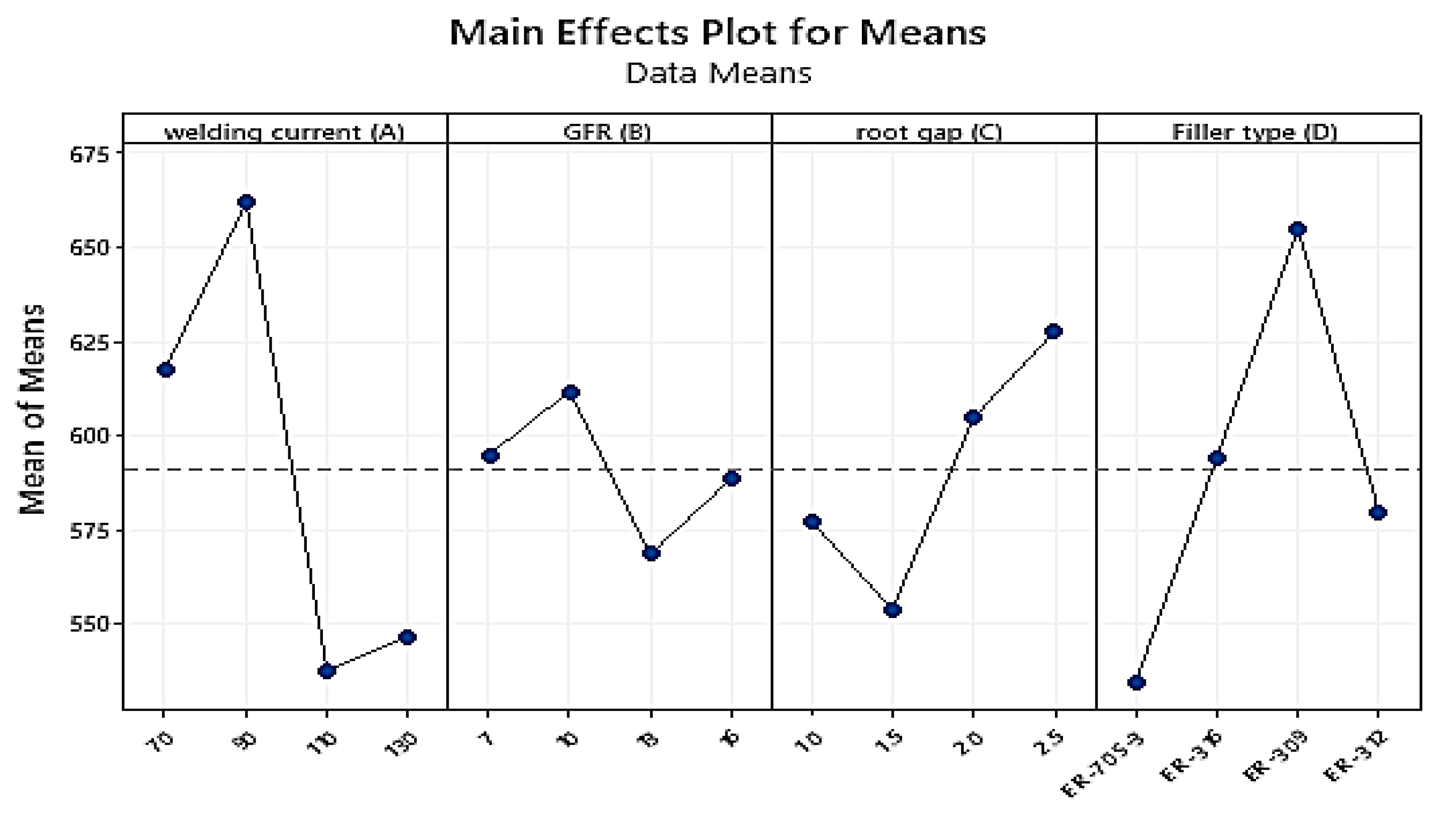
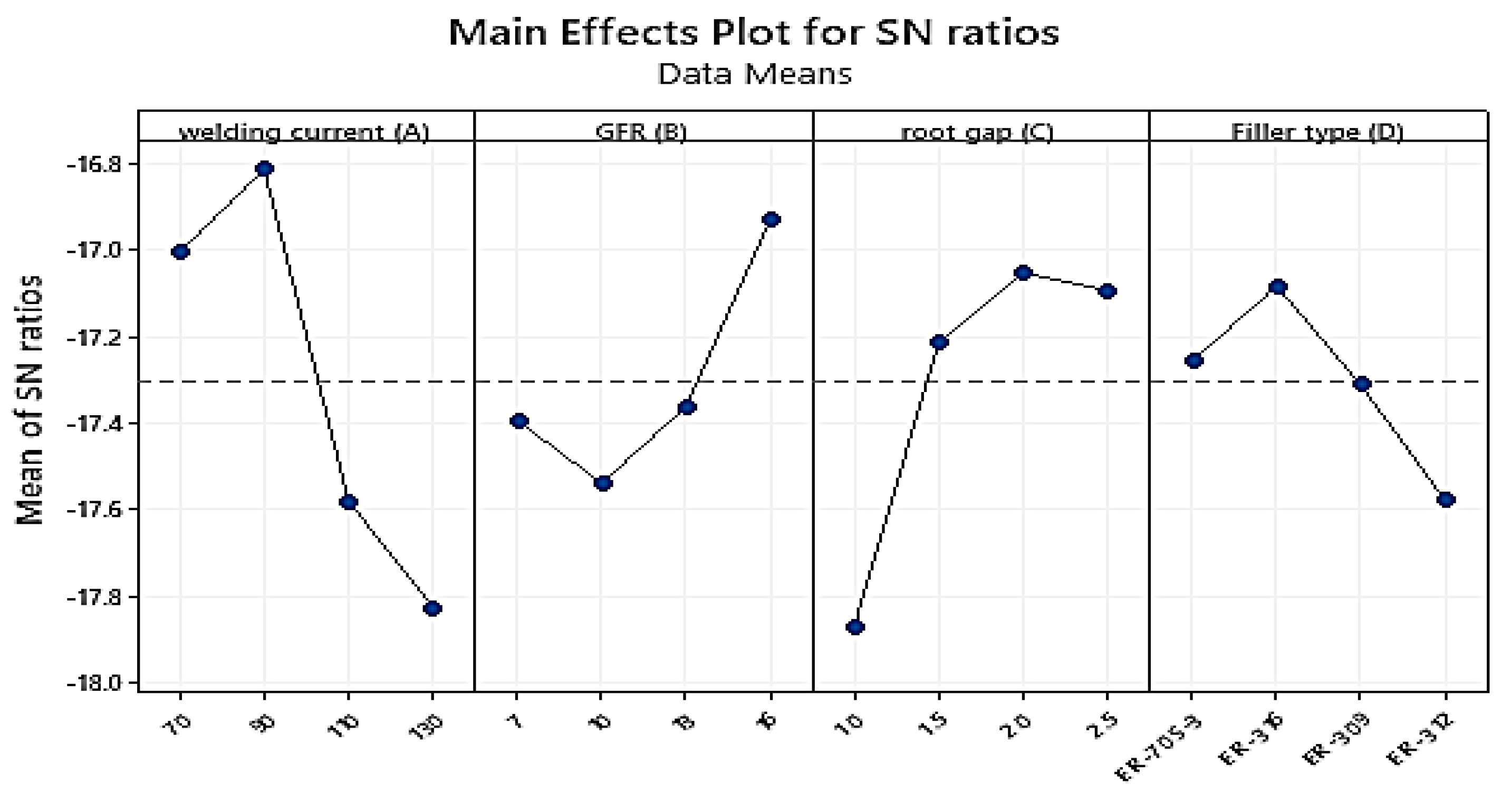
| 1 | 0.40013 | 0.31641 | 0.07283 | 0.20754 |
| 2 | 0.58009 | 0.39020 | 0.31232 | 0.37168 |
| 3 | 0.24503 | 0.36413 | 0.47585 | 0.47844 |
| 4 | 0.17859 | 0.33310 | 0.54284 | 0.34617 |
| Delta | 0.40150 | 0.07380 | 0.47001 | 0.27090 |
| Rank | 2 | 4 | 1 | 3 |
| Source | DF | Seq SS | % Cont. | Adj SS | Adj MS | F | P |
|---|---|---|---|---|---|---|---|
| welding current (A) | 3 | 0.38341 | 35 | 0.38341 | 0.127803 | 18.19 | 0.020 |
| GFR (B) | 3 | 0.01291 | 1.20 | 0.01291 | 0.004302 | 0.61 | 0.652 |
| root gap (C) | 3 | 0.52506 | 48 | 0.52506 | 0.175020 | 24.91 | 0.013 |
| Filler type (D) | 3 | 0.14909 | 14 | 0.14909 | 0.049697 | 7.07 | 0.071 |
| Residual Error | 3 | 0.02107 | 1.80 | 0.02107 | 0.007025 | ||
| Total | 15 | 1.09154 | 100 |
| Optimum Setting | UTS (MPa) | HARDNESS (HRB) | FS (MPa) | BW (mm) | CDI (dg) |
|---|---|---|---|---|---|
| A2 B2 C4 D3 | 493.2 | 86 | 691 | 5.8 | 0.9387 |
| Initial Setting | Optimum Setting | % Improvement | |||||||||
|---|---|---|---|---|---|---|---|---|---|---|---|
| A2 B4 C3 D2 | A2 B2 C4 D3 | ||||||||||
| UTS | HRD | FS | BW | UTS | HRD | FS | BW | UTS | HRD | FS | BW |
| 445 | 83 | 679 | 6.21 | 493.2 | 86 | 691 | 5.8 | 10.83 | 3.61 | 1.77 | 6.60 |
| Composite desirability | |||||||||||
| 0.7638 | 0.9387 | 22.90 | |||||||||
| Type of Samples | Optimum Setting | UTS (MPa) | HARDNESS (HRB) | FS (MPa) | BW (mm) | CDI (dg) | Error |
|---|---|---|---|---|---|---|---|
| Dissimilar | A2 B2 C4 D3 | 493.2 | 86 | 691 | 5.80 | 0.9387 | 3.42% |
| Exp. setting | 498 | 88 | 691.45 | 5.25 | 0.9708 | ||
| A2 B2 C4 D3 |
Publisher’s Note: MDPI stays neutral with regard to jurisdictional claims in published maps and institutional affiliations. |
© 2022 by the authors. Licensee MDPI, Basel, Switzerland. This article is an open access article distributed under the terms and conditions of the Creative Commons Attribution (CC BY) license (https://creativecommons.org/licenses/by/4.0/).
Share and Cite
Assefa, A.T.; Ahmed, G.M.S.; Alamri, S.; Edacherian, A.; Jiru, M.G.; Pandey, V.; Hossain, N. Experimental Investigation and Parametric Optimization of the Tungsten Inert Gas Welding Process Parameters of Dissimilar Metals. Materials 2022, 15, 4426. https://doi.org/10.3390/ma15134426
Assefa AT, Ahmed GMS, Alamri S, Edacherian A, Jiru MG, Pandey V, Hossain N. Experimental Investigation and Parametric Optimization of the Tungsten Inert Gas Welding Process Parameters of Dissimilar Metals. Materials. 2022; 15(13):4426. https://doi.org/10.3390/ma15134426
Chicago/Turabian StyleAssefa, Anteneh Teferi, Gulam Mohammed Sayeed Ahmed, Sagr Alamri, Abhilash Edacherian, Moera Gutu Jiru, Vivek Pandey, and Nazia Hossain. 2022. "Experimental Investigation and Parametric Optimization of the Tungsten Inert Gas Welding Process Parameters of Dissimilar Metals" Materials 15, no. 13: 4426. https://doi.org/10.3390/ma15134426
APA StyleAssefa, A. T., Ahmed, G. M. S., Alamri, S., Edacherian, A., Jiru, M. G., Pandey, V., & Hossain, N. (2022). Experimental Investigation and Parametric Optimization of the Tungsten Inert Gas Welding Process Parameters of Dissimilar Metals. Materials, 15(13), 4426. https://doi.org/10.3390/ma15134426