
Logistic Model of Phase Transformation of Hardening Concrete


Abstract
:1. Introduction
2. Materials and Methods
2.1. Characteristics of the Applied Materials
2.2. Investigation Methods of the Hardening Kinetics of Cementitious Materials
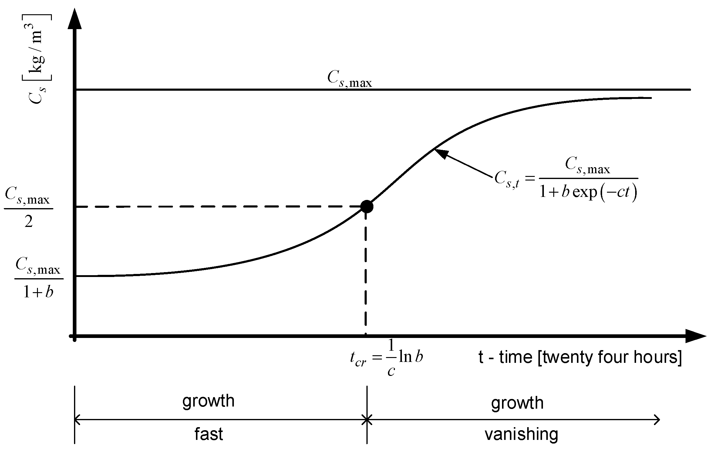
2.3. Mathematical Model
2.4. Validation of the Model
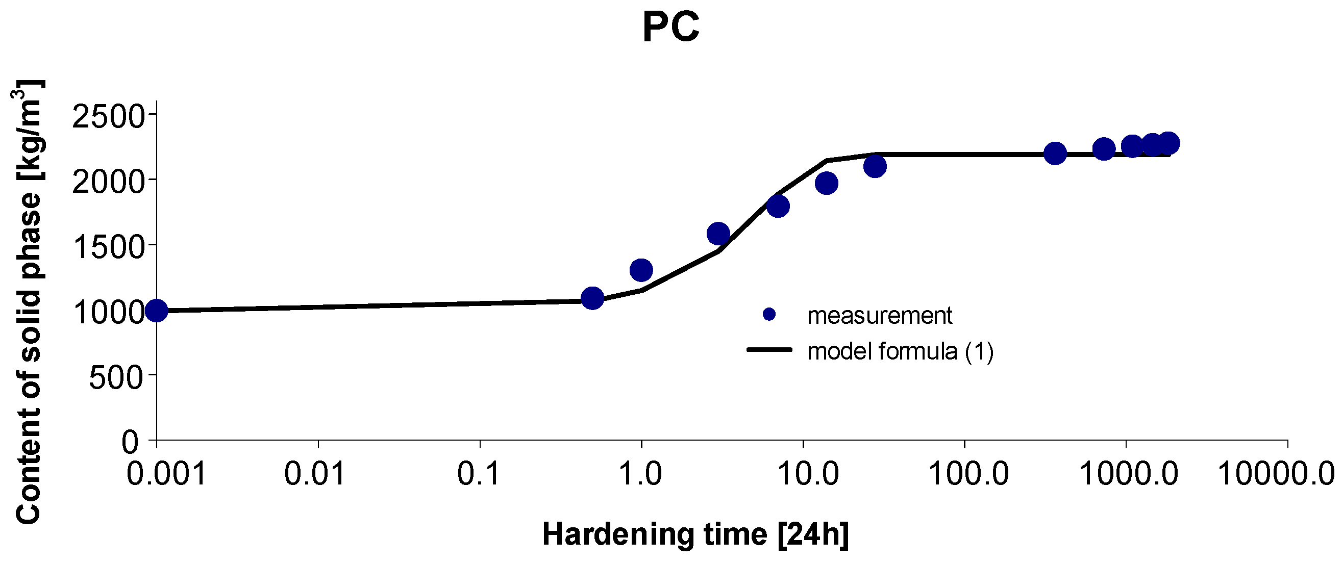
2.5. Concrete PC
3. Results and Discussion
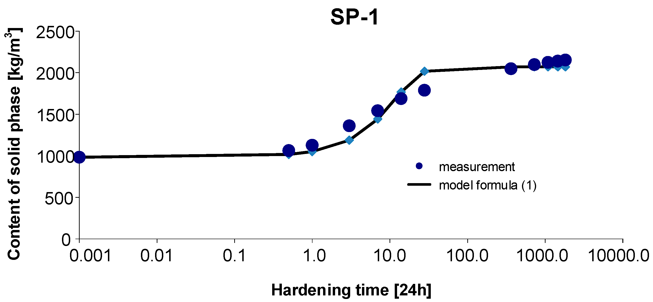
3.1. Materials SP-1
3.2. Materials SP-2
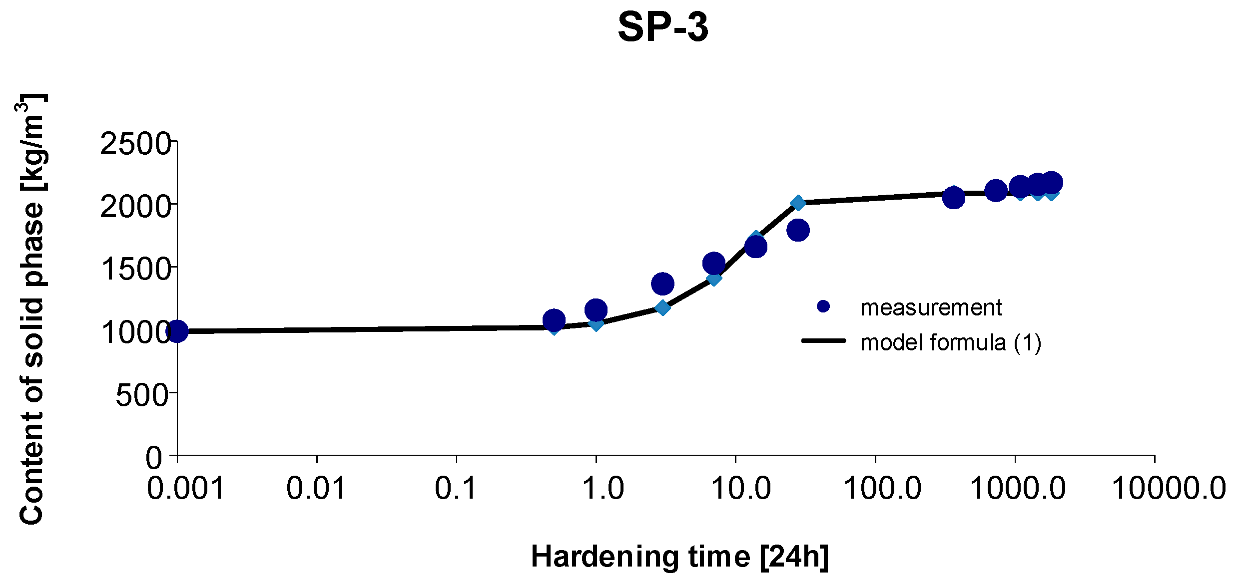
3.3. Materials SP-3
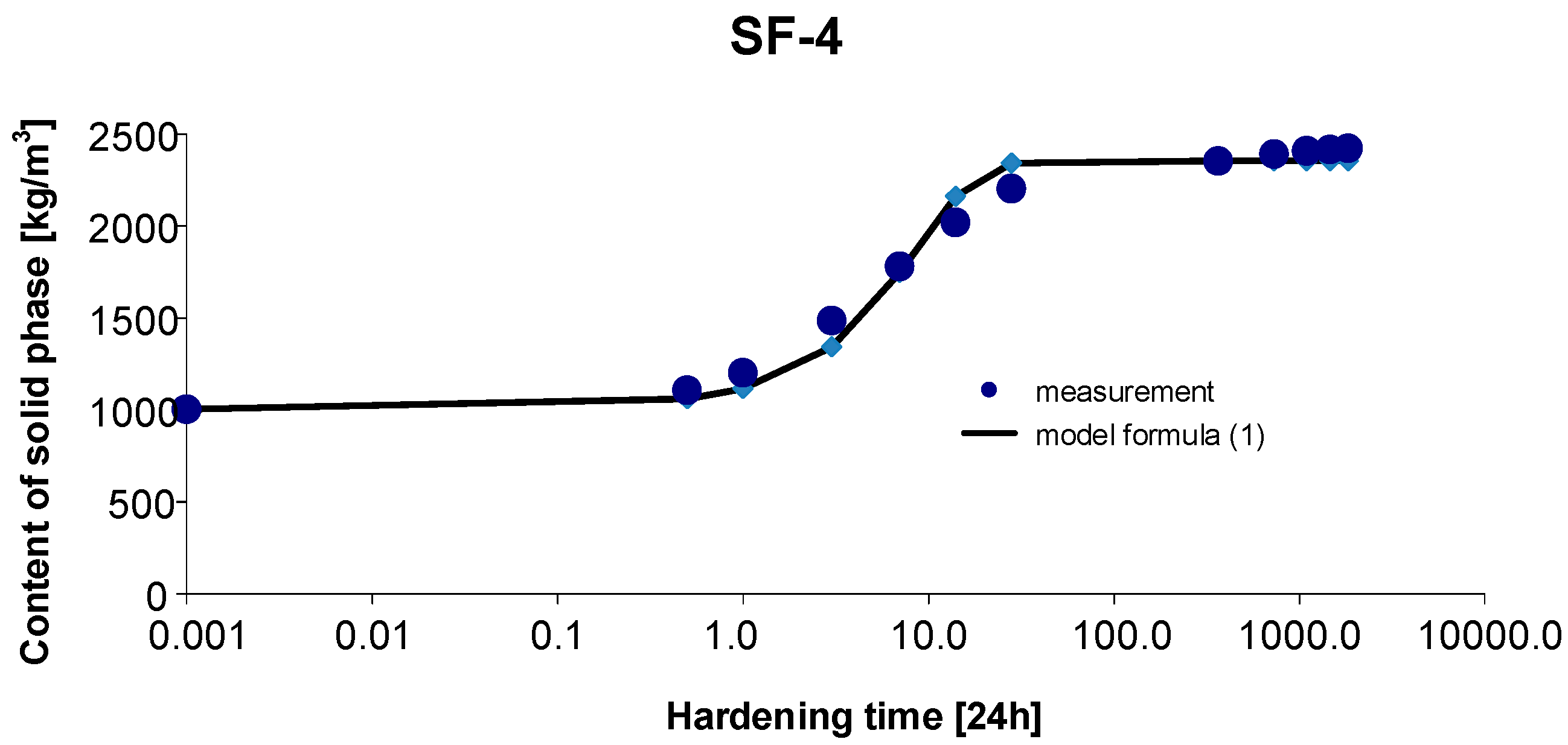
3.4. Materials SF-4
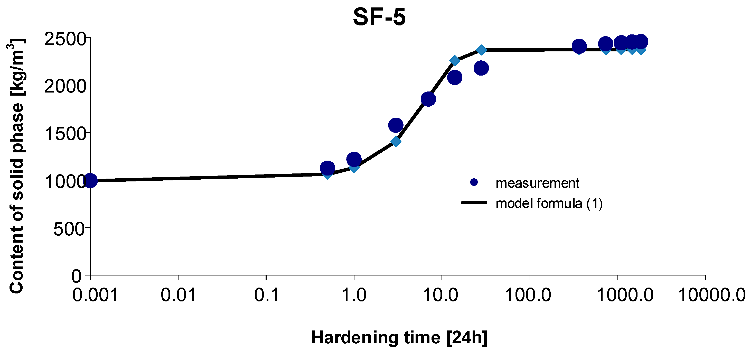
3.5. Materials SF-5
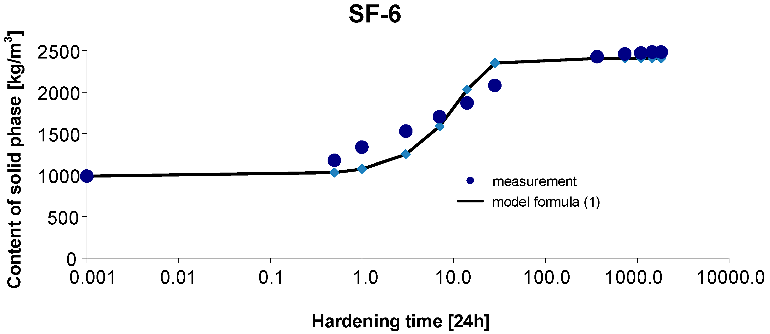
3.6. Materials SF-6
4. Conclusions
Author Contributions
Funding
Institutional Review Board Statement
Informed Consent Statement
Data Availability Statement
Conflicts of Interest
References
- Thai, M.Q.; Nguyen-Sy, J.; Wakim, M.N.; Vu, Q.D.; To, T.; Nguyen, T.T. A robust homogenization method for ageing and non-ageing viscoelastic behavior of early age and hardened cement pastes. Constr. Build. Mater. 2020, 264, 120264. [Google Scholar] [CrossRef]
- Allen, A.J.; Thomas, J.J.; Jennings, H.M. Composition and density of nanoscale calcium-silicate-hydrate in cement. Nat. Mater. 2007, 6, 311. [Google Scholar] [CrossRef] [PubMed]
- Bažant, Z.P.; Cusatis, G.; Codolin, L. Temperature effect on concrete creep modeled by microprestress-solidifaction theory. J. Eng. Mech. 2004, 130, 691–699. [Google Scholar] [CrossRef]
- Li, X.; Grasley, Z.C.; Garboczi, E.J.; Bulluard, J.W. Modeling the apparent and intrinsic viscoelastic relaxation of hydrating cement paste. Cem. Concr. Compos. 2015, 55, 322–330. [Google Scholar] [CrossRef]
- Mallick, S.; Anoop, M.B.; Rao, K.B. Early age creep of cement paste-Governing mechanisms and role of water—A microindentation study. Cem. Concr. Res. 2019, 116, 284–298. [Google Scholar] [CrossRef]
- Stefanidou, M.; Kamperidou, V.; Konstandinidis, A.; Koltsou, P.; Papadopoulos, S. 24-Rheological properties of biofibers in cementitious composite matrix. In Advances in Bio-Based Fiber Moving Towards a Green Society; The Textile Institute Book Series; Woodhead Publishing: Sawston, UK, 2022; pp. 553–573. [Google Scholar] [CrossRef]
- Zając, M.; Durdzinski, P.; Giergiczny, Z.; Ben Haha, M. New insights into the role of space on the microstructure and the development of strength of multicomponent cements. Cem. Concr. Comp. 2021, 121, 104070. [Google Scholar] [CrossRef]
- Skibsted, J.; Snellings, R. Reactivity of supplementary cementitious materials (SCMs) in cement blends. Cem. Concr.Res. 2019, 124, 105799. [Google Scholar] [CrossRef]
- Lotthenbach, B.; Scrivener, K.; Hooton, R.D. Supplementary cementitious materials. Cem. Concr. Res. 2011, 41, 1244–1256. [Google Scholar] [CrossRef]
- Artiolli, G.; Bullard, J.W. Cement hydratation: The role of adsorption and crystal growth. Cryst. Res. Technol. 2013, 48, 903–918. [Google Scholar] [CrossRef]
- Batóg, M.; Giergiczny, Z. Influence of mass concrete constituents on its properties. Constr. Build. Mater. 2017, 146, 221–230. [Google Scholar] [CrossRef]
- Bofang, Z. Thermal Stresses and Temperature Control of Mass Concrete; Butterworth-Heinemann: Oxford, UK, 2014. [Google Scholar]
- Xin, J.; Liu, L.; Jiang, Q.; Yang, P.; Qu, H.; Xie, G. Early-age hydratation characteristics of modified coal gasification slag-cement-aeolian sand paste backfill. Constr. Build. Mater. 2022, 322, 125936. [Google Scholar] [CrossRef]
- Zhao, Y.; Gao, J.; Chen, G.; Li, S.; Luo, X.; Xu, Z.; Guo, Z.; Du, H. Early-age hydratation characteristics and kinetics model of blended cement containing waste clay brick and slag. J. Build. Eng. 2022, 51, 104360. [Google Scholar] [CrossRef]
- Jiao, Z.; Wang, Y.; Zhen, G.W.; Huang, W. Effect of dosage of sodium carbonate on the strength and drying shrinkage of sodium hydroxide based alkali-activated slag paste. Constr. Build. Mater. 2018, 179, 11–24. [Google Scholar] [CrossRef]
- Wang, Y.; He, F.; Wang, J.; Wang, C.; Xiong, Z. Effects of calcium bicarbonate on the properties of plain Portland cement paste. Const. Build. Mater. 2019, 225, 591–600. [Google Scholar] [CrossRef]
- Li, L.; Chen, M.; Guo, X.; Lu, L.; Wang, S.; Cheng, X.; Wang, K. Early-age hydratation characteristics and kinetics of Portland cement pastes with super low w/c ratios using ice particles as mixing water. J. Mater. Res. Technol. 2020, 9, 8407–8428. [Google Scholar] [CrossRef]
- Li, W.; Fall, M. Sulphate effect on the early age strength and self-desiccation of cemented paste backfill. Constr. Build. Mater. 2016, 106, 296–304. [Google Scholar] [CrossRef]
- Nowoświat, A.; Gołaszewski, J. Influence of the variability of calcareous fly ash properties on rheological properties of fresh mortar with its addition. Materials 2019, 12, 1942. [Google Scholar] [CrossRef] [Green Version]
- Kim, S.; Son, H.M.; Park, S.; Lee, H.K. Effects of biological admixtures on hydratation and mechanical properties of Portland cement paste. Constr. Build. Mater. 2020, 235, 117461. [Google Scholar] [CrossRef]
- Chen, H.; Feng, P.; Ye, S.; Li, Q.; Hou, P.; Cheng, X. The influence of inorganic admixtures on early cement hydratation from the point of view of thermodynamics. Constr. Build. Mater. 2020, 259, 119777. [Google Scholar] [CrossRef]
- Jiang, H.; Fall, M.; Yilmaz, E.; Li, Y.; Yang, L. Effect on mineral admixtures on flow properties of fresh cemented paste backfill: Assessment of time dependency and thixotropy. Power Technol. 2020, 372, 258–266. [Google Scholar] [CrossRef]
- Zhang, N.; Yu, H.; Ma, H.; Ba, M. Effects of different pH chemical additives on the hydratation and hardening rules of basic magnesium sulfate cement. Constr. Build. Mater. 2021, 305, 124696. [Google Scholar] [CrossRef]
- Li, H.; Xue, Z.; Liang, G.; Wu, K.; Dong, B.; Wang, W. Effect of C-S-Hs-PCE and sodium sulfate on the hydratation kinetics and mechanical properties of cement paste. Constr. Build. Mater. 2021, 266, 121096. [Google Scholar] [CrossRef]
- Long, G.; Li, Y.; Ma, C.; Xie, Y.; Shi, Y. Hydratation kinetics of cement incorporating different nanoparticles at elevated temperatures. Thermochim. Acta 2018, 664, 108–117. [Google Scholar] [CrossRef]
- Wang, Y.; Lu, H.; Wang, J.; He, H. Effects of highly crystalized nano C-S-H particles on performances of Portland cement paste and its mechanism. Crystals 2020, 10, 816. [Google Scholar] [CrossRef]
- Schöler, A.; Lothenbach, B.; Winnefeld, F.; Haha, M.B.; Zając, M.; Ludwig, H.M. Early hydratation of SCM-blended Portland cements: A pore solution and isothermal calorimetry study. Cem. Concr. Res. 2017, 93, 71–82. [Google Scholar] [CrossRef]
- Zhai, M.; Zhao, J.; Wang, D.; Wang, Y.; Wang, Q. Hydratation properties and kinetic characteristics of blended cement containing lithium slag powder. J. Build. Eng. 2021, 39, 102287. [Google Scholar] [CrossRef]
- Ślusarek, J. The correlation of structure porosity and compressive strength of hardening cement materials. Archit. Civ. Eng. Environ. ACEE 2010, 3, 85–92. [Google Scholar]
- Ślusarek, J. The Cement Materials Hardening Model (Model Twardnienia Tworzyw Cementowych); Wydawnictwo Politechniki Śląskiej: Gliwice, Poland, 2001. (In Polish) [Google Scholar]
- Ślusarek, J. The theoretical fundamentals of heat and moisture transport in hardening concrete. Cem. Wapno Beton 2012, 17, 286–294. [Google Scholar]
- Stern, F.; Wilson, R.; Coleman, H.; Paterson, E.G. Comprehensive approach to verification and validation of CFD simulations—Part 1: Methodology and procedures. J. Fluids Eng. 2001, 123, 793–802. [Google Scholar] [CrossRef]
- Nowoświat, A.; Olechowska, M. Experimental validation of the model of reverberation time prediction in a room. Buildings 2022, 12, 347. [Google Scholar] [CrossRef]
- Schlesinger, S.; Crosbie, R.E.; Garagné, R.E.; Innis, G.S.; Lalwani, C.S.; Loch, J.; Sylvester, R.J.; Wright, R.D.; Kheir, N.; Bartos, D. Terminology for model credibility. Simulation 1979, 32, 103–104. [Google Scholar]


| Parameters | Type of Concrete Mixture | ||||||
|---|---|---|---|---|---|---|---|
| PC | SP-1 | SP-2 | SP-3 | SF-4 | SF-5 | SF-6 | |
| W/(C + SF) | 0.52 | 0.52 | 0.47 | 0.42 | 0.42 | 0.37 | 0.32 |
| C (kg/m3) | 340 | 345 | 363 | 394 | 320 | 348 | 388 |
| SF (kg/m3) | - | - | -- | 36 | 39 | 43 | |
| SP (kg/m3) | - | 4.310 | 4.540 | 4.925 | 8.900 | 9.675 | 10.781 |
| P (kg/m3) | 989 | 982 | 988 | 985 | 1003 | 992 | 988 |
| G (kg/m3) | 989 | 982 | 988 | 985 | 1003 | 992 | 988 |
| W (kg/m3) | 177 | 177 | 168 | 163 | 144 | 137 | 132 |
| ρB (kg/m3) | 2495 | 2490 | 2512 | 2532 | 2515 | 2518 | 2550 |
| ρSB (kg/m3) | 2519 | 2514 | 2533 | 2545 | 2552 | 2564 | 2577 |
| s (-) | 0.990 | 0.990 | 0.992 | 0.995 | 0.985 | 0.982 | 0.990 |
| j (-) | 0.001 | 0.001 | 0.008 | 0.005 | 0.015 | 0.018 | 0.010 |
| Va (dm3/m3) | 10 | 10 | 8 | 5 | 15 | 18 | 10 |
| Ve-Be (s) | 10.5 | 7.0 | 8.0 | 8.0 | 9.5 | 10.5 | 9.0 |
| fc, cube (MPa) after 28 days in hydroisolated condition (18 ± °C) | 50.4 | 53.5 | 63.7 | 77.8 | 77.7 | 86.4 | 93.5 |
| Parameters | Type of Concrete Mixture | ||||||
|---|---|---|---|---|---|---|---|
| PC | SP-1 | SP-2 | SP-3 | SF-4 | SF-5 | SF-6 | |
| CL,0 | 1506 | 1508.31 | 1523.54 | 1546.93 | 1511.9 | 1525.68 | 1561.78 |
| Cs,0 | 989 | 982 | 988 | 985 | 1003 | 992 | 988 |
| ρB | 2495 | 2490 | 2515 | 2532 | 2515 | 2518 | 2550 |
| Parameter | PC | SP-1 | SP-2 | SP-3 | SF-4 | SF-5 | SF-6 |
|---|---|---|---|---|---|---|---|
| αmax | 1.000 | 1.000 | 1.000 | 0.957 | 1.000 | 0.937 | 0.810 |
| xmax | 0.644 | 0.644 | 0.790 | 0.937 | 0.742 | 0.796 | 0.872 |
| Rmax (MPa) | 78.7 | 120.8 | 147.6 | 175.2 | 114.2 | 131.7 | 160.9 |
| R0 (MPa) | 125.11 | 187.26 | 187.26 | 187.26 | 251.16 | 251.16 | 251.16 |
| Hardening Time (24 h) | Degree of Conversion α (-) | ||||||
|---|---|---|---|---|---|---|---|
| PC | SP-1 | SP-2 | SP-3 | SF-4 | SF-5 | SF-6 | |
| 0.001 | 0 | 0 | 0 | 0 | 0 | 0 | 0 |
| 0.5 | 0.065 | 0.053 | 0.061 | 0.056 | 0.068 | 0.087 | 0.121 |
| 1 | 0.207 | 0.096 | 0.119 | 0.109 | 0.131 | 0.147 | 0.222 |
| 3 | 0.393 | 0.251 | 0.255 | 0.244 | 0.319 | 0.382 | 0.347 |
| 7 | 0.534 | 0.371 | 0.330 | 0.349 | 0.513 | 0.563 | 0.458 |
| 14 | 0.651 | 0.468 | 0.467 | 0.434 | 0.672 | 0.711 | 0.564 |
| 28 | 0.736 | 0.534 | 0.508 | 0.519 | 0.793 | 0.776 | 0.699 |
| 365 | 0.802 | 0.706 | 0.671 | 0.686 | 0.893 | 0.926 | 0.921 |
| 730 | 0.824 | 0.739 | 0.705 | 0.723 | 0.917 | 0.944 | 0.941 |
| 1095 | 0.839 | 0.757 | 0.721 | 0.742 | 0.929 | 0.951 | 0.950 |
| 1460 | 0.846 | 0.767 | 0.731 | 0.754 | 0.934 | 0.956 | 0.956 |
| 1825 | 0.854 | 0.776 | 0.743 | 0.763 | 0.939 | 0.959 | 0.956 |
| Parameters | Concrete Type | ||||||
|---|---|---|---|---|---|---|---|
| PC | SP-1 | SP-2 | SP-3 | SF-4 | SF-5 | SF-6 | |
| Cs,max | 2207.87 | 2104.02 | 2072.29 | 2125.44 | 2366.94 | 2388.06 | 2447.66 |
| Cs,mx/2 | 1103.94 | 1052.01 | 1036.14 | 1062.72 | 1183.47 | 1194.03 | 1223.82 |
| Cs,max/(1 + b) | 990.69 | 987.75 | 994.96 | 994.32 | 1095.20 | 1100.03 | 1217.78 |
| tcr | 0.742 | 1.007 | 0.969 | 1.203 | 0.937 | 0.853 | 0.117 |
Publisher’s Note: MDPI stays neutral with regard to jurisdictional claims in published maps and institutional affiliations. |
© 2022 by the authors. Licensee MDPI, Basel, Switzerland. This article is an open access article distributed under the terms and conditions of the Creative Commons Attribution (CC BY) license (https://creativecommons.org/licenses/by/4.0/).
Share and Cite
Ślusarek, J.; Nowoświat, A.; Olechowska, M. Logistic Model of Phase Transformation of Hardening Concrete. Materials 2022, 15, 4403. https://doi.org/10.3390/ma15134403
Ślusarek J, Nowoświat A, Olechowska M. Logistic Model of Phase Transformation of Hardening Concrete. Materials. 2022; 15(13):4403. https://doi.org/10.3390/ma15134403
Chicago/Turabian StyleŚlusarek, Jan, Artur Nowoświat, and Marcelina Olechowska. 2022. "Logistic Model of Phase Transformation of Hardening Concrete" Materials 15, no. 13: 4403. https://doi.org/10.3390/ma15134403
APA StyleŚlusarek, J., Nowoświat, A., & Olechowska, M. (2022). Logistic Model of Phase Transformation of Hardening Concrete. Materials, 15(13), 4403. https://doi.org/10.3390/ma15134403