
Hot Ductility Prediction Model of Cast Steel with Low-Temperature Transformed Structure during Continuous Casting


Abstract
1. Introduction
2. Materials
2.1. Data Collection
2.2. Data Preprocessing
2.2.1. Data Normalization
2.2.2. Data Filtering
3. Methods
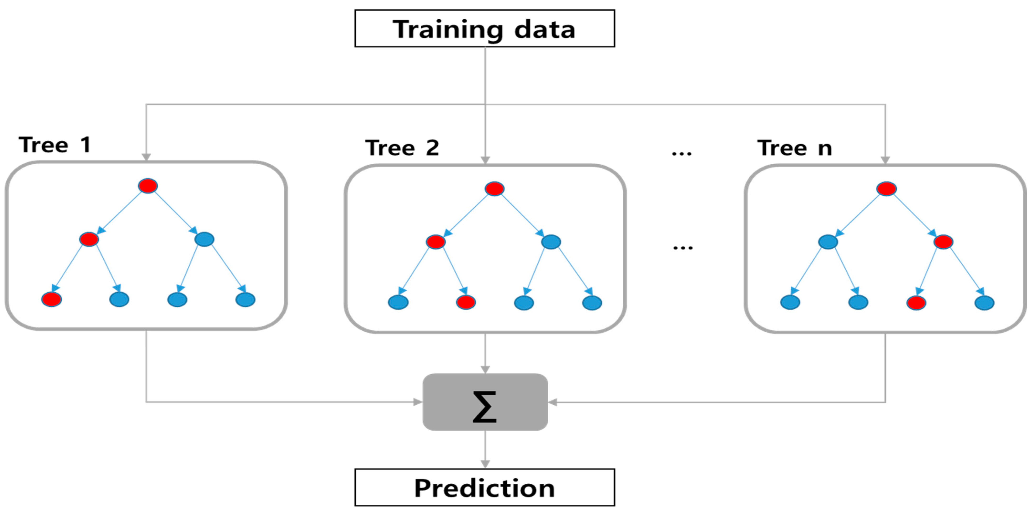
3.1. RF
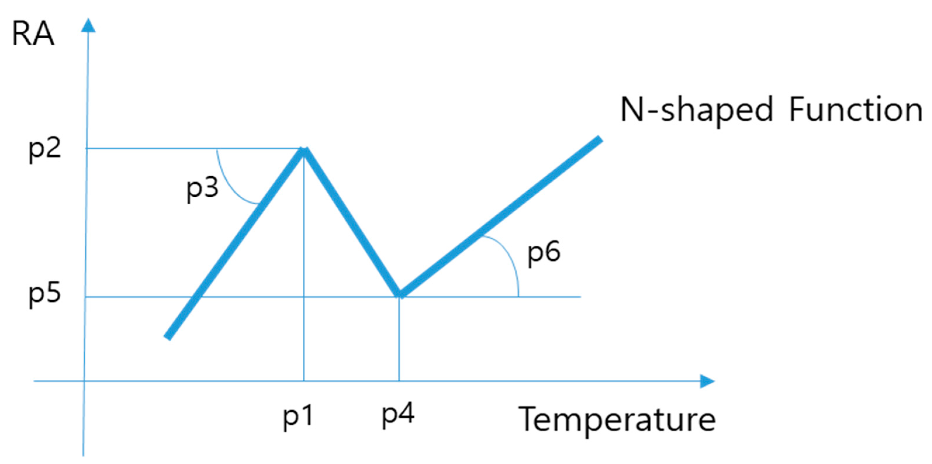
3.2. N-Shaped Data Filtering
3.3. Model Optimization and Performance Metrics
4. Result and Discussion
4.1. Prediction Results Using RF Model
4.2. Evaluation of Prediction Performance among Four Machine Learning Models
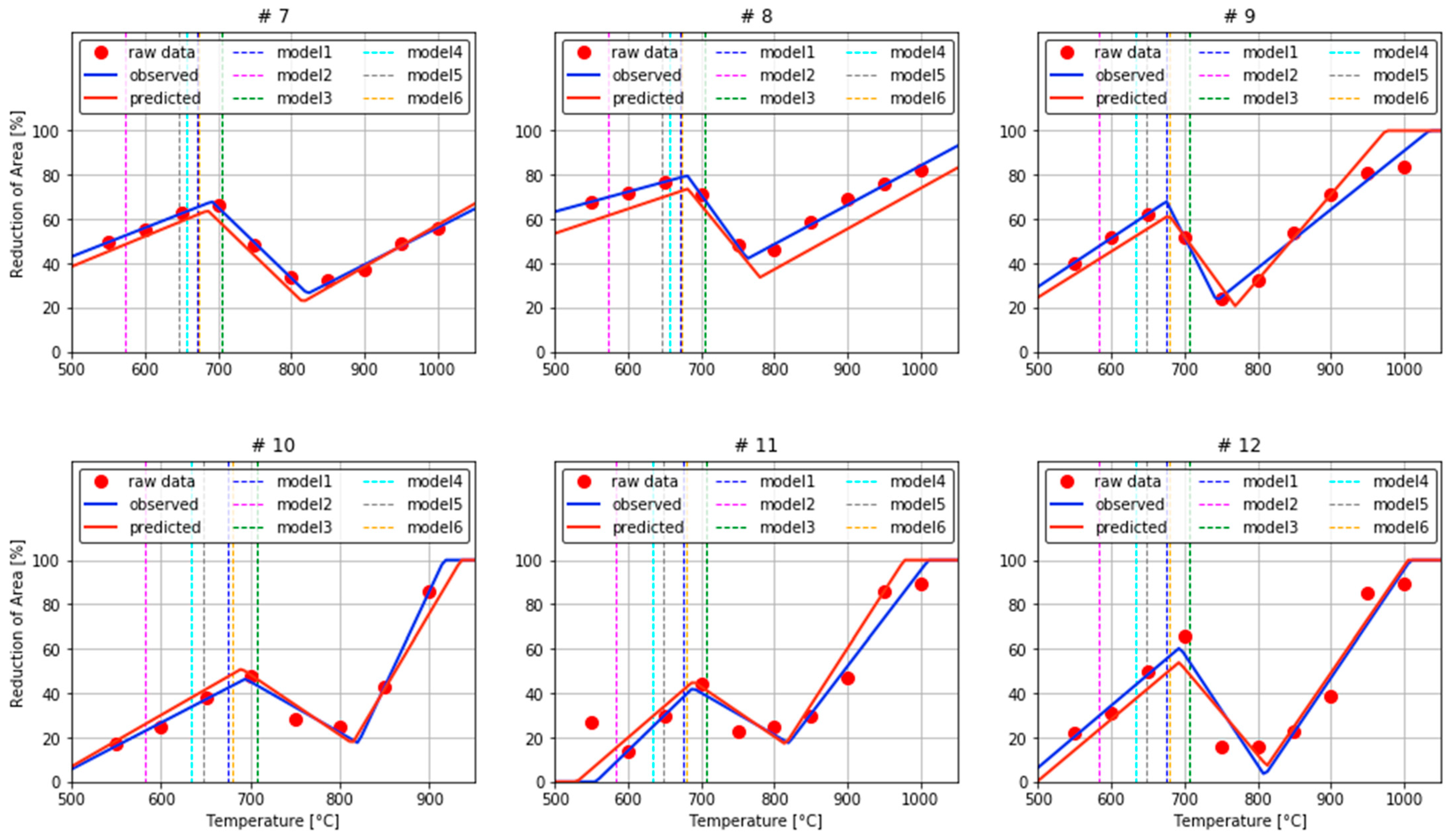
4.3. Prediction of Bainite Start Temperature in Alloy Steel
4.4. Comparison of RA Behavior between Gaussian and N-Fitting Model of Nb-Added Steel
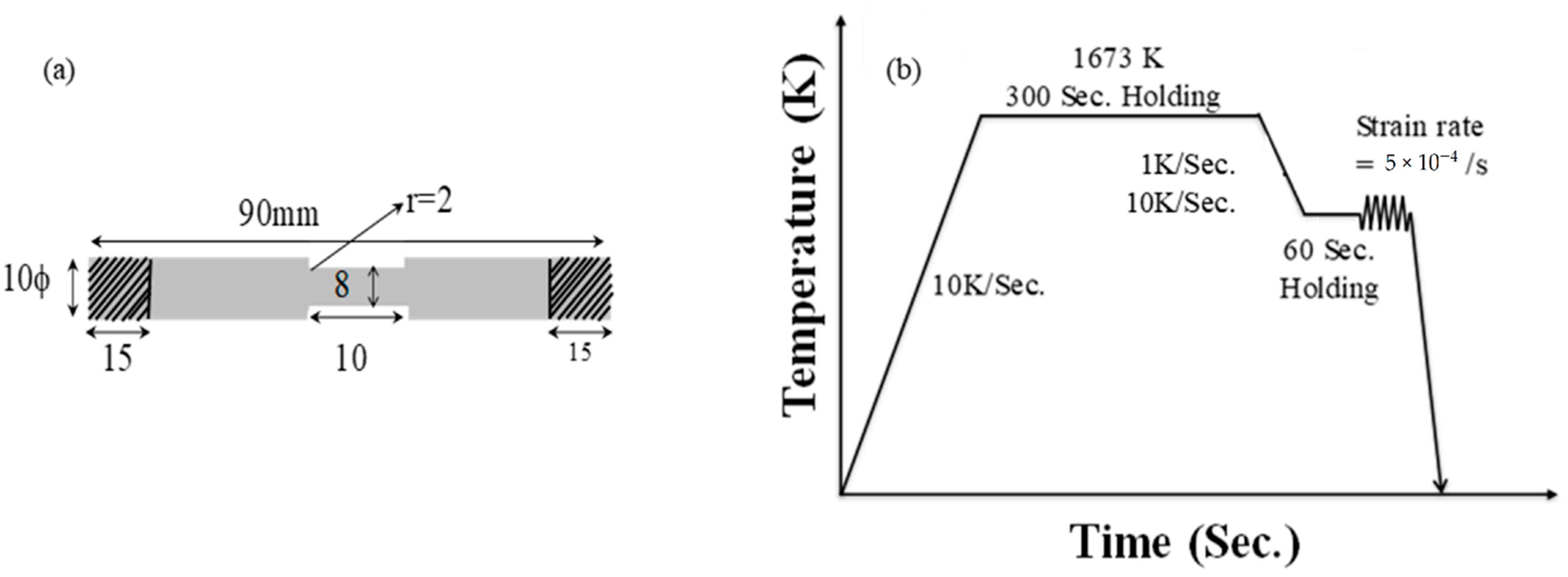
4.4.1. Experimental Procedure
4.4.2. Analysis of Result
5. Conclusions
Author Contributions
Funding
Institutional Review Board Statement
Informed Consent Statement
Data Availability Statement
Conflicts of Interest
Appendix A
| Authors | Source | Publication (Year, Volume, Page) |
| Byoungchul Hwang et al. | Materials Science | 2005, 402, 177 |
| UnHae Lee et al. | ISIJ International | 2010, 50, 540 |
| KyungChul Cho et al. | Metallurgical and Materials Transactions A | 2010, 41, 1421 |
| Chihiro Nagasaki and Junji Kihara | ISIJ International | 1997, 37, 523 |
| Guoyu Qian et al. | ISIJ International | 2014, 54, 1611 |
| Hirowo G. Suzki et al. | ISIJ International | 1984, 24, 169 |
| Xia Jiang and Shenhua Song | Materials Science and Engineering A | 2014, 613, 171 |
| Jessica Calvo et al. | ISIJ International | 2007, 47, 1518 |
| William T. Nactrab and Yu T. Chou | Metallurgical Transactions A | 1986, 17, 1995 |
| Israel Mejía et al. | Materials Science and Engineering: A | 2011, 528, 4468 |
| Edgar L. Chipres et al. | Materials Science and Engineering: A | 2007, 460, 464 |
| Zakaria Mohhamed | Materials Science and Engineering: A | 2002, 326, 255 |
| Atef S. Hamada and Pentti Karjalainen | Materials Science and Engineering: A | 2011, 528, 1819 |
| Chiaki Ouhi and Kazuaki Matsumoto | ISIJ International | 1982, 22, 181 |
| Junru Li et al. | Materials Science and Engineering: A | 2016, 677, 274 |
| Thierry Rewaux et al. | ISIJ International | 1994, 34, 528 |
| Hang Su et al. | Materials Science and Technology | 2013, 23, 1357 |
| Weijian Liu et al. | ISIJ International | 2015, 56, 1133 |
| Barrie Mintz | ISIJ International | 1999, 39, 833 |
| ShinEon Kang et al. | Materials Science and Technology | 2021, 37, 42 |
| Lesley H. Choun and Lesley A. Cornish | Materials Science and Engineering: A | 2008, 494, 263 |
| Nowak Wolańska et al. | J. Achievements Mater. Manuf. Eng. | 2007, 20, 291 |
| Abdelbaset M. Elwazri et al. | ISIJ International | 1999, 39, 253- |
| Lesley H. Choun | Ph.D. Thesis, University of the Witwatersrand | 2008 |
| Kristin R. Capenter | Ph.D. Thesis, University of Wollongong | 2004 |
| Haiwen Luo et al. | ISIJ International | 2002, 42, 273 |
| Yasuhiro Maehara and Yasuya Ohmori | Materials Science and Engineering | 1984, 62, 109 |
| David Crother et al. | Metallurgical Transactions A | 1987, 18, 1929 |
| Nils E. Hannerrs | Transactions of the Iron and Steel Institute of Japan | 1985 |
| Brendan M. Connolly | Ph.D. Thesis, University of Pittsburgh | 2016 |
| Kevin M. Banks et al. | International Journal of Metallurgical Engineering | 2013, 2, 188 |
| Kevin M. Banks et al. | Materials Science and Technology | 2012, 28, 536 |
| Zuhair Mohjamed | Ph.D. Thesis, City University London | 1988 |
| Zuhair Mohjamed | Engineering Journal of University of Qatar | 1995, 8, 167 |
| KyungChul Cho | Ph.D. Thesis, Pohang University of Science and Technology | 2011 |
| Yaxu Zheng et al., | Materials Science and Engineering: A | 2018, 715, 194 |
| Yutian He et al. | Materials Science and Engineering: A | 2016, 673, 99 |
| Xiao-Min Chen et al. | Materials Science and Engineering: A | 2010, 527, 2725 |
| Shenhua Song et al. | Journal of Rare Earths | 2016, 34, 1062 |
| Shenhua Song et al. | Materials Science and Engineering: A | 2003, 360, 96 |
| Jessica Carlvo et al. | Engineering Failure Analysis | 2007, 14, 374 |
| Chang-Hoon Lee et al. | Materials Science and Engineering: A | 2016, 651, 192 |
| Faramarz Zarandi and Steve Yue | ISIJ International | 2006, 46, 591 |
| Xue Jiang et al. | Materials Science and Engineering: A | 2013, 574, 46 |
| Shenhua Song et al. | Materials Science and Engineering: A | 2014, 595, 188 |
| SangChul Seo et al. | Metals and Materials International | 2006, 12, 273 |
| Shin Eon Kang | Ph.D. Thesis, City University London | 2014 |
| Jingyu Li and Guoguang Cheng | Journal of Materials Research and Technology | 2020, 9, 52 |
| Cheng-bin Shi et al. | Materials Transactions | 2016, 57, 647 |
| Eduardo H. Delgado and Rodolfo D. Morales | Metallurgical and Materials Transactions B volume | 2001, 32, 919 |
| Ramesses Abusosha et al. | Materials Science and Technology | 1999, 15, 278 |
| Monica L. Wang et al. | Kang T’ieh/Iron and Steel | 2012 |
| Andrew Cowley et al. | Materials Science and Technology | 1998, 14, 1145 |
| Ramesses Abusosha et al. | Materials Science and Technology | 1998, 14, 346 |
| Ramesses Abusosha et al. | Materials Science and Technology | 1998, 14, 227 |
| Barrie Mintz et al. | Materials Science and Technology | 1998, 14, 222 |
| Barrie Mintz et al. | Materials Science and Technology | 1995, 11, 474 |
| Barrie Mintz and Ramesses Abushosha | Materials Science and Technology | 1992, 8, 171 |
| Ramesses Abusosha et al. | Materials Science and Technology | 1991, 7, 613 |
| Chen L. Zhen et al. | Steel Research | 1990, 61, 620 |
| Barri Mintz and Mike Arrowsmith | Metals Technology | 1979, 6, 24 |
| Chas Spradery and Barrie Mintz | Ironmaking & Steelmaking | 2005, 32, 319 |
| Prasonk Sricharoenchai et al. | ISIJ International | 1992, 32, 1102 |
| Kyung-Chul Cho et al. | ISIJ International | 2010, 50, 839 |
| Barrie Mintz et al. | International Materials Reviews | 1991, 36, 187 |
| Barrie Mintz et al. | Materials Science and Technology | 2003, 19, 1721 |
| Mustafa M. Arıkan | Metals | 2015, 5, 986 |
| Hirowo G. Susuki et al. | ISIJ International | 1982, 22, 48 |
| Chunyu He et al. | Metals | 2020, 10, 1679 |
References
- Brimacombe, J.K. The challenge of quality in continuous casting processes. Metall. Mater. Trans. A 1999, 30, 1899–1912. [Google Scholar] [CrossRef]
- Mintz, B.; Yue, S.; Jonas, J.J. Hot ductility of steels and its relationship to the problem of transverse cracking during continuous casting. Int. Mater. Rev. 1991, 36, 187–220. [Google Scholar] [CrossRef]
- Kamada, Y.; Hashimoto, T.; Watanabe, S. Effect of Hot Charge Rolling Condition on Mechanical Properties of Nb Bearing Steel Plate. ISIJ Int. 1990, 30, 241–247. [Google Scholar] [CrossRef][Green Version]
- Zhao, J.; Wang, W.; Liu, Q.; Wang, Z.; Shi, P. A two-stage scheduling method for hot rolling and its application. Control. Eng. Pract. 2009, 17, 629–641. [Google Scholar] [CrossRef]
- Min, J.H.; Heo, Y.U.; Kwon, S.H.; Moon, S.W.; Kim, D.G.; Lee, J.S.; Yim, C.H. Embrittlement mechanism in a low-carbon steel at intermediate temperature. Mater. Charact. 2019, 149, 34–40. [Google Scholar] [CrossRef]
- Yamanaka, A.; Nakajima, K.; Okamura, K. Critical strain for internal crack formation in continuous casting. Ironmak. Steelmak. 1995, 22, 508–512. [Google Scholar]
- Suzuki, K.; Miyagawa, S.; Saito, Y. Effect of microalloyed nitride forming elements on precipitation of carbonitride and high temperature ductility of continuously cast low carbon Nb containing steel slab. ISIJ Int. 1995, 35, 34–41. [Google Scholar] [CrossRef]
- Vedani, M.; Ripamonti, D.; Mannucci, A. Hot ductility of microalloyed steels. La Metallurg. Italy 2008, 100, 19–24. [Google Scholar]
- Maehara, Y.; Nakai, K.; Yasumoto, K. Hot cracking of low alloy steels in simulated continuous casting-direct rolling process. Trans. Iron Steel Inst. Jpn. 1998, 28, 1021–1027. [Google Scholar] [CrossRef]
- Hong, D.; Kwon, S.; Yim, C. Exploration of Machine Learning to Predict Hot Ductility of Cast Steel from Chemical Composition and Thermal Conditions. Met. Mater. Int. 2021, 27, 298–305. [Google Scholar] [CrossRef]
- Abushosha, R.; Ayyad, S.; Mintz, B. Influence of cooling rate on hot ductility of C-MN-Al and C-MN-Nb-Al steels. Mater. Sci. Technol. 1998, 14, 227–235. [Google Scholar] [CrossRef]
- Sismanis, P. Modeling solidification phenomena in the continuous casting of carbon steels. In Two Phase Flow, Phase Change and Numerical Modeling; Ahsan, A., Ed.; InTech: London, UK, 2011; pp. 122–148. [Google Scholar]
- Spradbery, C.; Mintz, B. Influence of undercooling thermal cycle on hot ductility of C–Mn–Al–Ti and C–Mn–Al–Nb–Ti steels. Ironmak. Steelmak. 2005, 32, 319–324. [Google Scholar] [CrossRef]
- Liu, Q.; Zhang, X.; Wang, B. Control technology of solidification and cooling in the process of continuous casting of steel. In Science and Technology of Casting Processes; Srinivasan, M., Ed.; InTech: London, UK, 2012; pp. 169–203. [Google Scholar]
- Sterjovski, Z.; Nolan, D.; Carpenter, K.R. Artificial neural networks for modelling the mechanical properties of steels in various applications. J. Mater. Process. Technol. 2005, 170, 536–544. [Google Scholar] [CrossRef]
- Kwon, S.H.; Hong, D.G.; Yim, C.H. Prediction of hot ductility of steels from elemental composition and thermal history by deep neural networks. Ironmak. Steelmak. 2020, 47, 1176–1187. [Google Scholar] [CrossRef]
- Zhang, Y.; Yu, L.; Fu, T.; Wang, J.; Shen, F.; Cui, K. Microstructure evolution and growth mechanism of Si-MoSi2 composite coatings on TZM (Mo-0.5Ti-0.1Zr-0.02C) alloy. J. Alloy. Compd. 2022, 894, 162403. [Google Scholar] [CrossRef]
- Patro, S.; Sahu, K. Normalization: A preprocessing stage. arXiv 2015, arXiv:1503.06462. [Google Scholar] [CrossRef]
- Xu, Z.W.; Liu, X.M.; Zhang, K. Mechanical properties prediction for hot rolled alloy steel using convolutional neural network. IEEE Access 2019, 7, 47068–47078. [Google Scholar] [CrossRef]
- Brieman, L. Random Forests. Mach. Learn. 2001, 45, 5–23. [Google Scholar] [CrossRef]
- Géron, A. Hands-On Machine Learning with Scikit-Learn and TensorFlow, Sebastopol; O’Reilly Media: Sebastopol, CA, USA, 2017. [Google Scholar]
- Dangeti, P. Statistics for Machine Learning; Packt Publishing Ltd.: Birmingham, UK, 2017. [Google Scholar]
- Kemmer, G.; Keller, S. Nonlinear least-squares data fitting in Excel spreadsheets. Nat. Protoc. 2010, 5, 267–281. [Google Scholar] [CrossRef]
- Müller, P.; Parmigiani, G. Optimal Design via Curve Fitting of Monte Carlo Experiments. J. Am. Stat. Assoc. 1995, 90, 1322–1330. [Google Scholar]
- Boyd, S.; Vandenberghe, L. Convex Optimization; Cambridge University Press: Cambridge, UK, 2004. [Google Scholar]
- Leung, M.K.; Yang, Y.H. Dynamic two-strip algorithm in curve fitting. Pattern Recognit. 1990, 23, 69–79. [Google Scholar] [CrossRef]
- Svetnik, V.; Liaw, A.; Tong, C.; Culberson, J.C.; Sheridan, R.P.; Feuston, B.P. Random Forest: A Classification and Regression Tool for Compound Classification and QSAR Modeling. J. Chem. Inf. Model. 2003, 43, 1947–1958. [Google Scholar] [CrossRef] [PubMed]
- Kelley, K.; Lai, K. Accuracy in Parameter Estimation for the Root Mean Square Error of Approximation: Sample Size Planning for Narrow Confidence Intervals. Multivar. Behav. Res. 2012, 46, 1–32. [Google Scholar] [CrossRef] [PubMed]
- Bergstra, J.; Bengio, Y. Random search for hyper-parameter optimization. J. Mach. Learn. Res. 2012, 13, 281–305. [Google Scholar]
- Boulesteix, A.L.; Janitza, S.; Kruppa, J.; König, I.R. Overview of random forest methodology and practical guidance with emphasis on computational biology and bioinformatics. Data Min. Knowl. Discov. 2012, 2, 493–507. [Google Scholar] [CrossRef]
- Bernard, S.; Heutte, L.; Adam, S. Influence of hyperparameters on random forest accuracy. In MCS, Vol. 5519 of Lecture Notes in Computer Science; Springer: Berlin/Heidelberg, Germany, 2009; pp. 171–180. [Google Scholar]
- Rodriguez, J.D.; Perez, A.; Lozano, J.A. Sensitivity Analysis of k-Fold Cross Validation in Prediction Error Estimation. IEEE Trans. Pattern Anal. Mach. Intell. 2010, 32, 569–575. [Google Scholar] [CrossRef]
- Jung, Y.S. Multiple predicting K-fold cross-validation for model selection. J. Nonparametric Stat. 2018, 30, 197–215. [Google Scholar] [CrossRef]
- Ranganathan, A.; Yang, M.; Ho, J. Online Sparse Gaussian Process Regression and Its Applications. IEEE Trans. Image Process. 2011, 20, 391–404. [Google Scholar] [CrossRef]
- Wang, B.; Chen, T. Gaussian process regression with multiple response variables. Chemometr. Intell. Lab. Syst. 2015, 142, 159–165. [Google Scholar] [CrossRef]
- Gu, B.; Sheng, V.S.; Wang, Z.; Ho, D.; Osman, S.; Li, S. Incremental learning for ν-Support Vector Regression. Neural Netw. 2015, 67, 140–150. [Google Scholar] [CrossRef]
- Tuia, D.; Verrelst, J.; Alonso, L.; Perez-Cruz, F.; Camps-Valls, G. Multioutput Support Vector Regression for Remote Sensing Biophysical Parameter Estimation. IEEE Geosci. Remote Sens. Lett. 2011, 8, 804–808. [Google Scholar] [CrossRef]
- Tang, J.; Deng, C.; Huang, G. Extreme Learning Machine for Multilayer Perceptron. IEEE Trans. Neural Netw. Learn. Syst. 2016, 27, 809–821. [Google Scholar] [CrossRef] [PubMed]
- Abiodun, O.I.; Jantan, A.; Omolara, A.E.; Dada, K.V.; Mohamed, N.A.; Arshad, H. State-of-the-art in artificial neural network applications: A survey. Heliyon 2018, 4, e00938. [Google Scholar] [CrossRef] [PubMed]
- Edmons, D.V.; Cochrane, R.C. Structure-property relationships in bainitic steels. Metall. Trans. A 1990, 2, 1527–1540. [Google Scholar] [CrossRef]
- Stevens, W.; Haynes, A.G. The Temperature of Formation of Martensite and Bainite in Low-Alloy Steels. J. Iron Steel Inst. 1956, 183, 349–359. [Google Scholar]
- Kirkaldy, J.S.; Venugopalan, D. Phase Transformations in Ferrous Alloys; Marder, A.R., Goldstein, J.I., Eds.; TMS-AIME: Warrendale, PA, USA, 1984; pp. 125–167. [Google Scholar]
- Suehiro, M.; Senuma, T.; Yada, H.; Matsumura, Y.; Ariyoshi, T. A kinetic model for phase transformations of low carbon steels during continuous cooling. Tetsu-to-Hagané 1987, 73, 1026–1033. [Google Scholar] [CrossRef]
- Bodnar, R.L.; Ohhashi, T.; Jaffee, R.I. Effects of Mn, Si, and Purity on the Design of 3.5NiCrMoV, 1CrMov, and 2.25Cr-1Mo Bainitic Alloy Steels. Metall. Trans. A 1989, 20, 1445–1460. [Google Scholar] [CrossRef]
- Zhao, J. Continuous cooling transformations in steels. Mater. Sci. Technol. 1992, 8, 997–1004. [Google Scholar]
- Kunitake, T.; Okada, Y. The estimation of bainite transformation References temperatures in steels by the empirical formulas. J. Iron Steel Inst. 1998, 84, 137–141. [Google Scholar] [CrossRef]
- Lee, J.K. Prediction of Tensile Deformation Behavior of Formable Hot Rolled Steels; POSCO Technical Research Laboratories Report; POSCO: Pohang, Korea, 1999. [Google Scholar]
- Zhao, J.; Liu, C.; Liu, Y.; Northwood, D.O. A new empirical formula for the bainite upper temperature limit of steel. J. Mater. Sci. 2001, 36, 5045–5056. [Google Scholar] [CrossRef]
- Lee, Y.K. Empirical Formula of Isothermal Bainite Start Temperature of Steels. J. Mat. Sci. Let. 2002, 21, 1253–1255. [Google Scholar] [CrossRef]
- Bohemen, S.M.C. Bainite and martensite start temperature calculated with exponential carbon dependence. Mater. Sci. Technol. 2012, 28, 487–495. [Google Scholar] [CrossRef]


| Chemical | Minimum | Maximum | Thermal History | Minimum | Maximum | Unit |
|---|---|---|---|---|---|---|
| Component | ||||||
| C | 0.001 | 0.52 | Heating Temperature | 1250 | 1500 | °C |
| Si | 0 | 0.425 | Heat Holding Time | 120 | 300 | s |
| Mn | 0 | 1.9 | Cooling Rate | 0 | 10 | °C/s |
| P | 0 | 0.11 | Cool Holding Time | 0 | 300 | s |
| S | 0 | 0.015 | Strain Rate | 0.0001 | 0.02 | 1/s |
| Cu | 0 | 1 | ||||
| Nb | 0 | 0.078 | ||||
| Ni | 0 | 1 | ||||
| Al | 0 | 0.41 | ||||
| Mo | 0 | 0.093 | ||||
| N | 0 | 0.016 | ||||
| Cr | 0 | 1.1 | ||||
| V | 0 | 0.35 | ||||
| Ti | 0 | 0.054 | ||||
| B | 0 | 0.005 | ||||
| Sn | 0 | 0.192 |
| Steel | Component | ||||||
|---|---|---|---|---|---|---|---|
| C | Si | Mn | P | S | Nb | Al | |
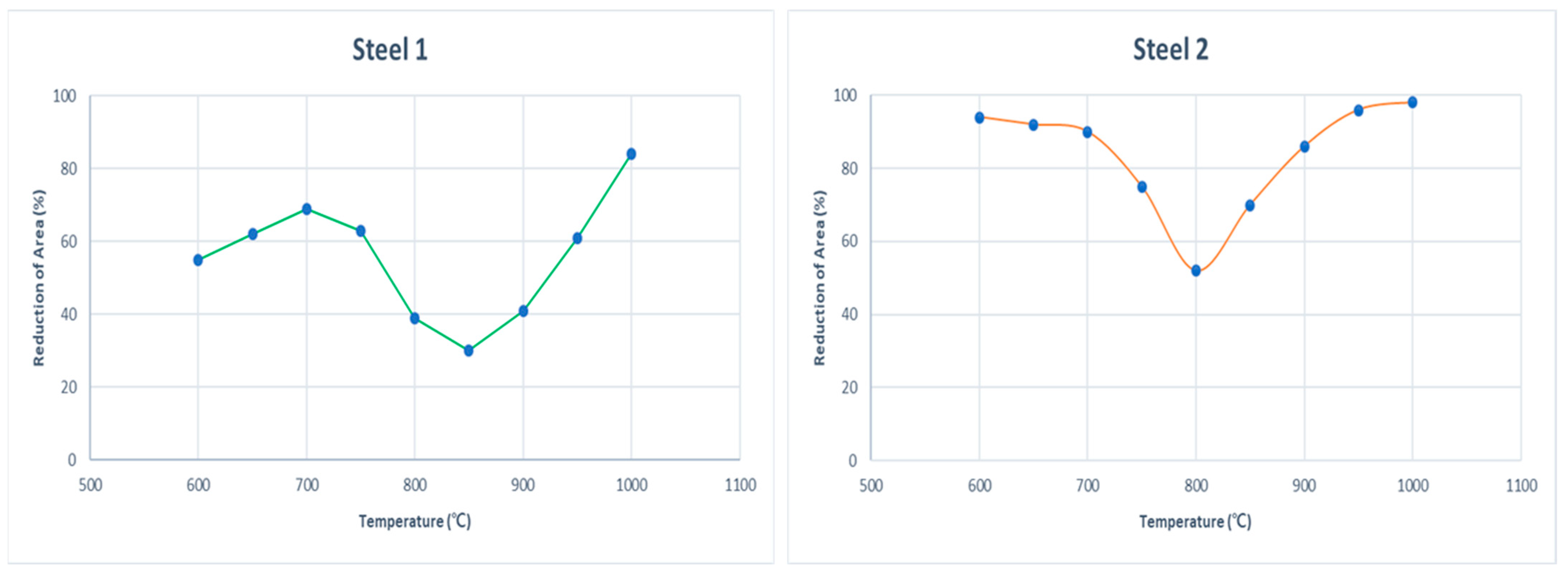
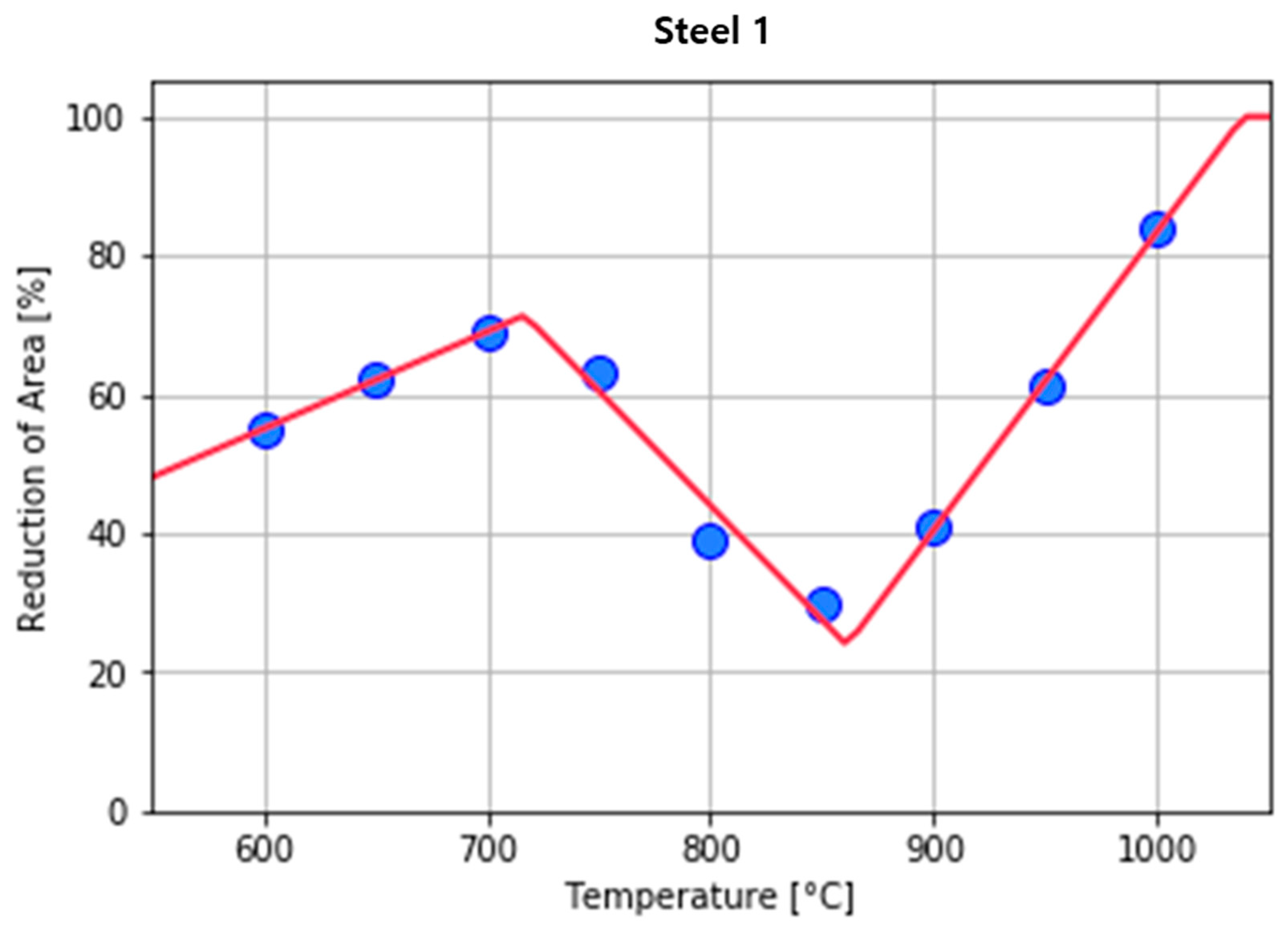
| Steel 1 | 0.09 | 0.01 | 0.01 | 0.002 | - | 0.07 | - |
| Steel 2 | 0.09 | 0.23 | 1.40 | 0.007 | 0.002 | 0.02 | 0.03 |
| Model | RMSE | |||||
|---|---|---|---|---|---|---|
| p1 | p2 | p3 | p4 | p5 | p6 | |
| RF | 11.10 | 5.11 | 0.056 | 15.20 | 6.11 | 0.075 |
| GPR | 19.22 | 9.975 | 0.103 | 28.01 | 4.903 | 0.156 |
| SVR | 29.57 | 10.66 | 0.132 | 32.96 | 12.34 | 0.156 |
| ANN | 71.89 | 15.95 | 0.272 | 58.40 | 29.97 | 0.174 |
| No. | Equation | Reference |
|---|---|---|
| 1 | Bs = 830 − 270C − 90Mn − 37Ni − 70Cr − 83Mo | [41] |
| 2 | Bs = 656 − 57.7C − 75Si − 35Mn − 15.3Ni − 34Cr − 41.2Mo | [42] |
| 3 | Bs = 844 − 597C − 63Mn − 16Ni − 78Cr | [44] |
| 4 | Bs = 732 − 202C + 216Si − 85Mn − 37Ni − 47Cr − 39Mo | [46] |
| 5 | Bs = 745 − 110C − 59Mn − 39Ni − 68Cr − 106Mo + 17MnNi + 6Cr2 + 29Mo2 | [49] |
| 6 | Bs = 839 − 270[1 − exp(−1.33C)] − 86Mn − 23Si − 67Cr − 33Ni − 75Mo | [50] |
| Bs Temperature | RMSE | ||||||
|---|---|---|---|---|---|---|---|
| Model 1 | Model 2 | Model 3 | Model 4 | Model 5 | Model 6 | RFR | |
| P1 | 51.44 | 97.60 | 87.64 | 55.87 | 42.90 | 47.70 | 11.10 |
| Steel | Component | ||||||
|---|---|---|---|---|---|---|---|
| C | Si | Mn | P | S | Nb | Cu | |
| Steel | 0.16 | 0.3 | 0.15 | 0.01 | 0.005 | 0.01 | 0.03 |
Publisher’s Note: MDPI stays neutral with regard to jurisdictional claims in published maps and institutional affiliations. |
© 2022 by the authors. Licensee MDPI, Basel, Switzerland. This article is an open access article distributed under the terms and conditions of the Creative Commons Attribution (CC BY) license (https://creativecommons.org/licenses/by/4.0/).
Share and Cite
Hong, D.-G.; Kwon, S.-H.; Yim, C.-H. Hot Ductility Prediction Model of Cast Steel with Low-Temperature Transformed Structure during Continuous Casting. Materials 2022, 15, 3513. https://doi.org/10.3390/ma15103513
Hong D-G, Kwon S-H, Yim C-H. Hot Ductility Prediction Model of Cast Steel with Low-Temperature Transformed Structure during Continuous Casting. Materials. 2022; 15(10):3513. https://doi.org/10.3390/ma15103513
Chicago/Turabian StyleHong, Dae-Geun, Sang-Hum Kwon, and Chang-Hee Yim. 2022. "Hot Ductility Prediction Model of Cast Steel with Low-Temperature Transformed Structure during Continuous Casting" Materials 15, no. 10: 3513. https://doi.org/10.3390/ma15103513
APA StyleHong, D.-G., Kwon, S.-H., & Yim, C.-H. (2022). Hot Ductility Prediction Model of Cast Steel with Low-Temperature Transformed Structure during Continuous Casting. Materials, 15(10), 3513. https://doi.org/10.3390/ma15103513