
Modeling Structural Dynamics Using FE-Meshfree QUAD4 Element with Radial-Polynomial Basis Functions


Abstract
1. Introduction
2. Shape Functions for FE-RPIM QUAD4 Element
2.1. Formulation of Shape Functions
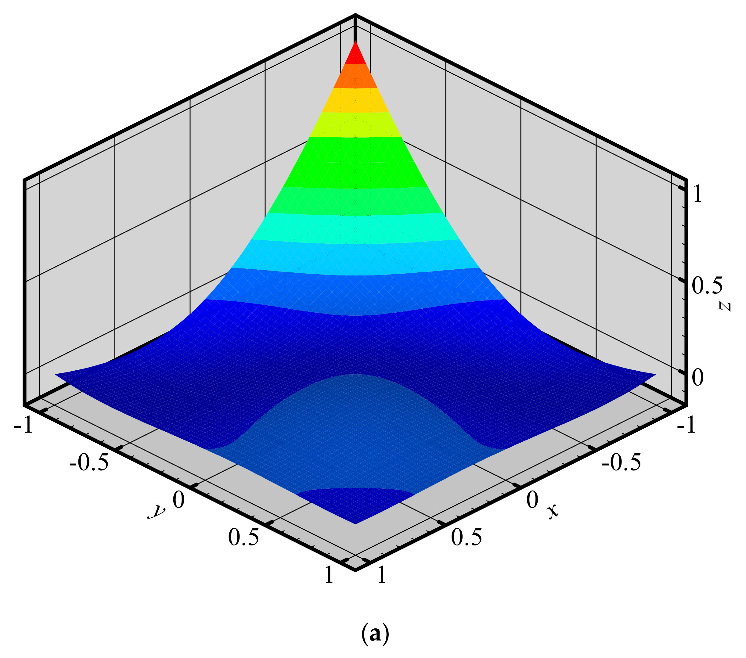
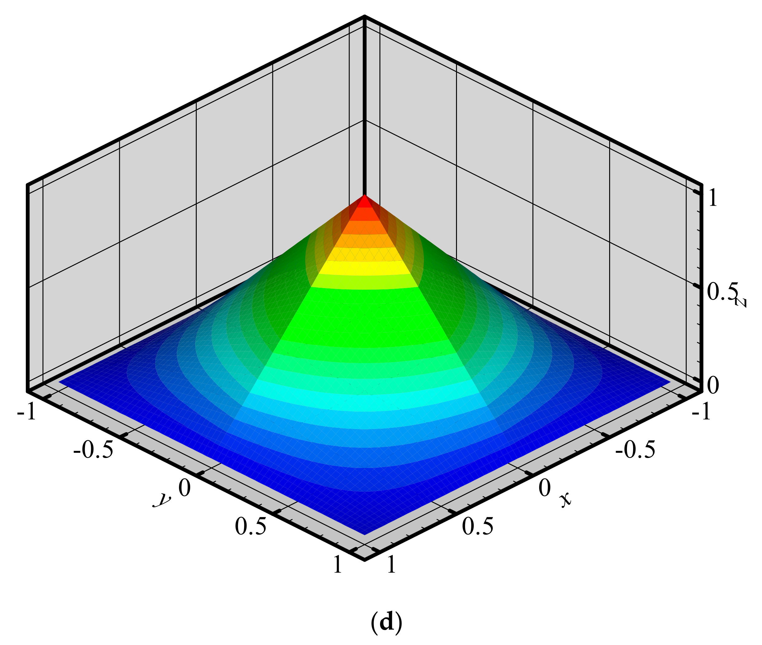
2.2. Properties of Shape Functions
- (i)
- Kronecker-delta character
- (ii)
- Compatibility property at the interface of elements.
- (iii)
- High order completeness, in other words, reproducibility of all the assumed Cartesian terms (Equation (3)).
3. FE-RPIM QUAD4 for Elastodynamic Problems
3.1. FE-RPIM QUAD4 for Dynamic Analysis
3.2. Time Integration Scheme
3.3. Generalized Eigenvalue Problem
3.4. Diagonally Lumped Mass Matrix
4. Numerical Examples
4.1. Cook’s Skew Beam
4.2. A Slender Rod
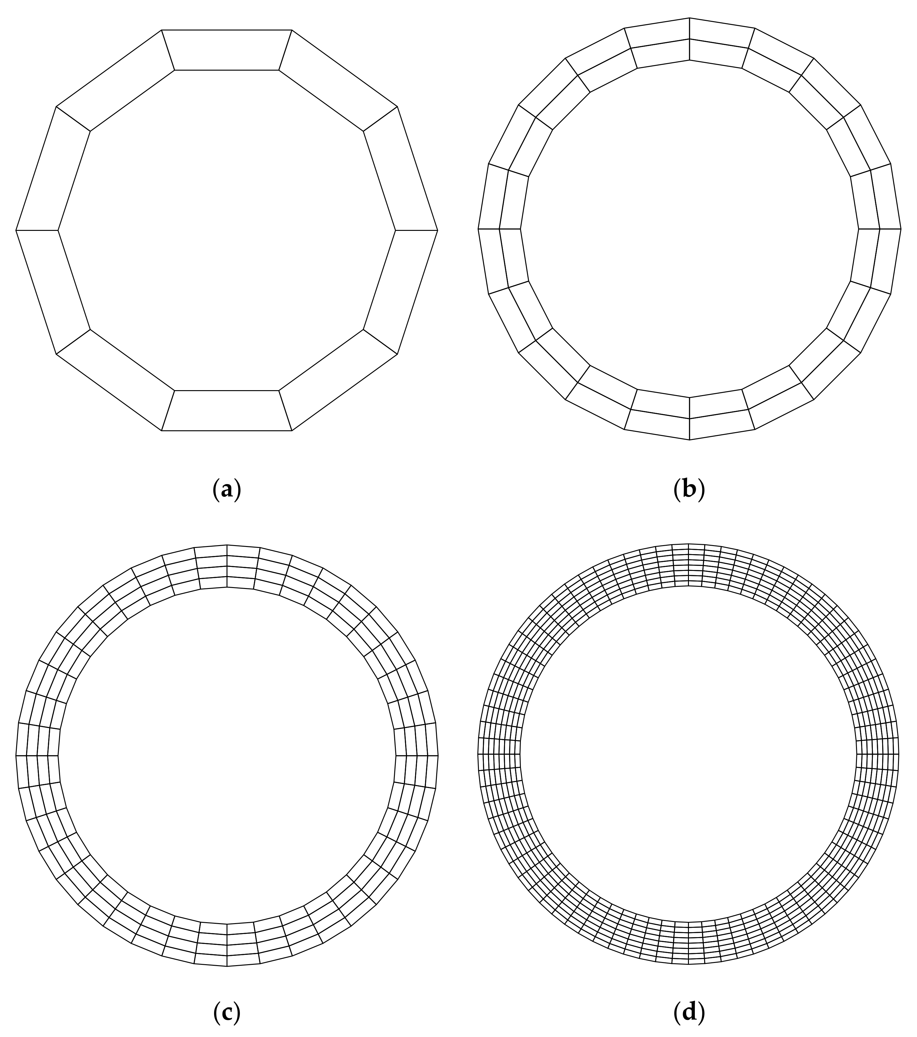
4.3. An Annulus
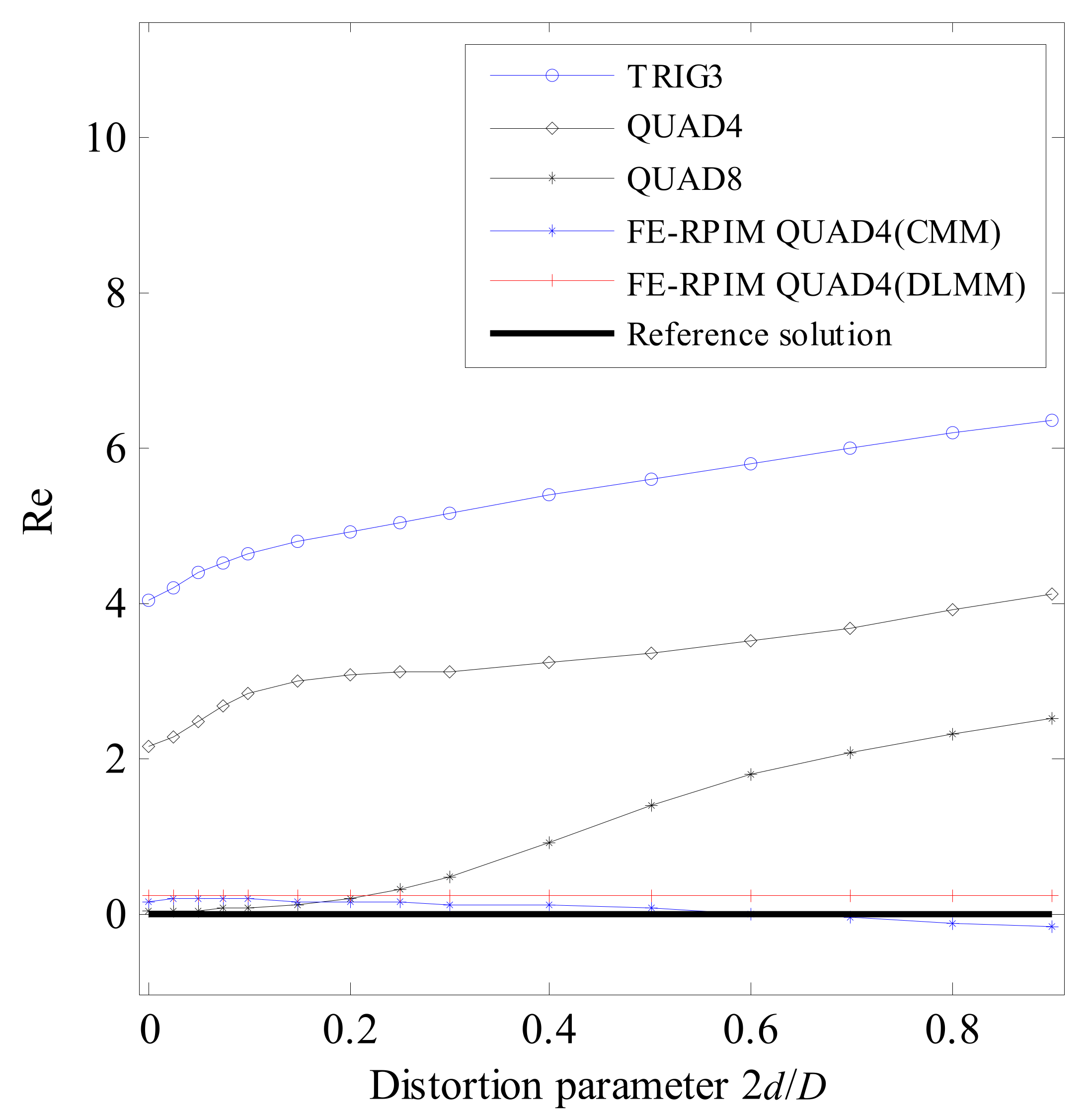
4.4. Mesh Distortion Test
- (1)
- First, as distortion parameter’s value increases, the errors based on FE-RPIM QUAD4 element do not change appreciably, while those based on QUAD4 element, TRIG3 element and QUAD8 elements change rapidly. The FE-RPIM QUAD4 element is immune to mesh distortion.
- (2)
- Second, accuracy of FE-RPIM QUAD4 element is always much higher than QUAD4 and TRIG3 elements.
- (3)
- Third, when 2d/D < 0.2, QUAD8 element’s accuracy is higher than QUAD4, FE-RPIM QUAD4 and TRIG3 elements. However, as the value of 2d/D increases, accuracy through QUAD8 element deteriorates quickly. If meshes used are distorted severely, QUAD8 element’s accuracy is much lower than FE-RPIM QUAD4 element.
- (4)
- Fourth, compared to CMM, FE-RPIM QUAD4 element can achieve better results if DLMM is employed.
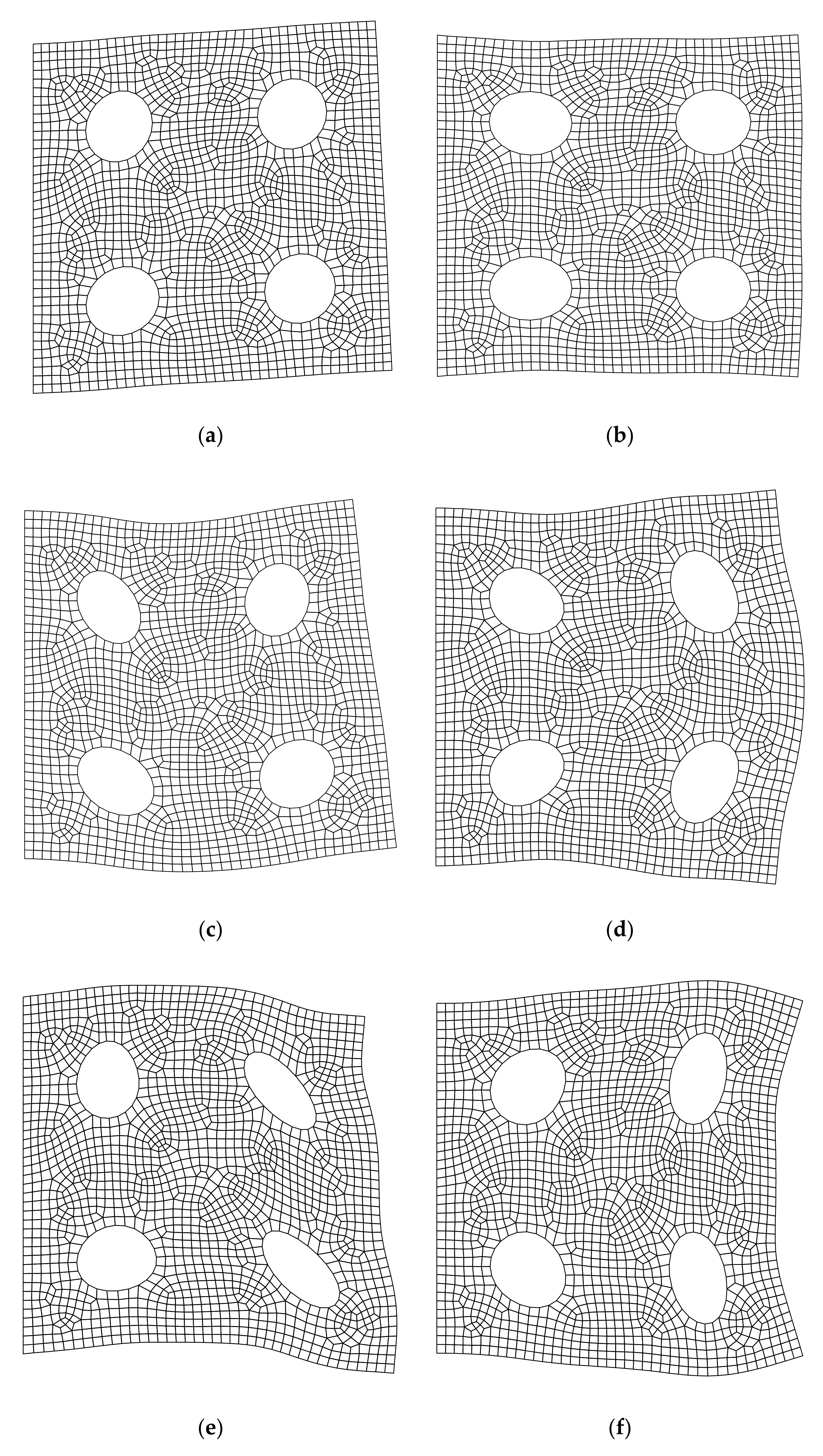
4.5. A Plate with Four Holes
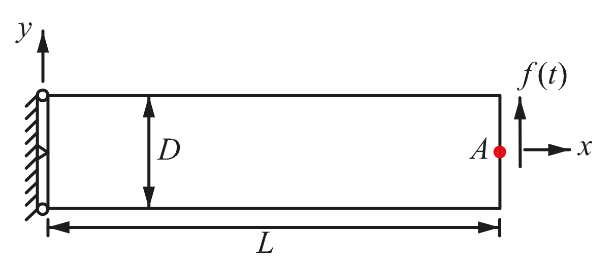
4.6. A Cantilever Beam under Harmonic Load
5. Conclusions
- (1)
- Based on 4-node quadrilateral mesh, FE-RPIM QUAD4 element’s accuracy is much higher than QUAD4 and TRIG3 elements (Table 2).
- (2)
- Although FE-RPIM QUAD4 element’s accuracy is slightly inferior to QUAD8 element, QUAD8 element requires more nodes than FE-RPIM QUAD4 element to discretize the problem domain. In addition, FE-RPIM QUAD4 element can achieve results closing to the reference solution, even for coarse mesh (Figure 22).
- (3)
- For distorted meshes, FE-RPIM QUAD4 element’s accuracy is always much higher than QUAD4 and TRIG3 elements. Moreover, FE-RPIM QUAD4 element is immune to mesh distortion, but TRIG3, QUAD4 and QUAD8 elements give very bad results as the mesh quality deteriorates (Figure 14).
- (4)
- In the tests associated to the analysis of free vibration, the result based on the DLMM are very close to those based on the CMM in the context of FE-RPIM QUAD4 element. In the test on forced vibration analysis, the result from the DLMM also agrees well with that from the CMM, which means DLMM can supersede the CMM in the context of the FE-RPIM QUAD4 element even for the scheme of implicit time integration.
Author Contributions
Funding
Institutional Review Board Statement
Informed Consent Statement
Data Availability Statement
Conflicts of Interest
References
- Reddy, J.N. An Introduction to Nonlinear Finite Element Analysis; Oxford University Press: Oxford, UK, 2004. [Google Scholar]
- Song, C. The scaled boundary finite element method in structural dynamics. Int. J. Numer. Methods Eng. 2009, 77, 1139–1171. [Google Scholar] [CrossRef]
- Kim, Y.; Ha, S.; Chang, F.K. Time-domain spectral element method for built-in piezoelectric-actuator-induced lamb wave propagation analysis. Aiaa J. 2008, 46, 591–600. [Google Scholar] [CrossRef]
- He, S.; Ng, C.T. A probabilistic approach for quantitative identification of multiple delaminations in laminated composite beams using guided waves. Eng. Struct. 2016, 127, 602–614. [Google Scholar] [CrossRef]
- Yeung, C.; Ng, C.T. Time-domain spectral finite element method for analysis of torsional guided waves scattering and mode conversion by cracks in pipes. Mech. Syst. Signal Process. 2019, 128, 305–317. [Google Scholar] [CrossRef]
- Nagashima, T. Node-by-node meshless approach and its application to structural analyses. Int. J. Numer. Methods Eng. 1999, 46, 341–385. [Google Scholar] [CrossRef]
- Lucy, L.B. A numerical approach to the testing of the fission thesis. Astron. J. 1977, 82, 1013–1024. [Google Scholar] [CrossRef]
- Nayroles, B.; Touzot, G.; Villon, P. Generating the finite element method: Diffuse approximation and diffuse elements. Comput. Mech. 1992, 10, 307–318. [Google Scholar] [CrossRef]
- Belytschko, T.; Lu, Y.Y.; Gu, L. Element-free Galerkin method. Int. J. Numer. Methods Eng. 1994, 37, 229–256. [Google Scholar] [CrossRef]
- Zhuang, X.Y.; Augarde, C. Aspects of the use of orthogonal basis functions in the element free Galerkin method. Int. J. Numer. Methods Eng. 2010, 81, 366–380. [Google Scholar] [CrossRef]
- Rabczuk, T.; Belytschko, T.; Xiao, S.P. Stable particle methods based on Lagrangian kernels. Comput. Methods Appl. Mech. Eng. 2004, 193, 1035–1063. [Google Scholar] [CrossRef]
- Cai, Y.C.; Zhu, H.H. A meshless local natural neighbour interpolation method for stress analysis of solids. Eng. Anal. Bound. Elem. 2004, 28, 607–613. [Google Scholar]
- Liu, G.R.; Gu, Y.T. A point interpolation method for two dimensional solid. Int. J. Numer. Methods Eng. 2001, 50, 937–951. [Google Scholar] [CrossRef]
- Liu, G.; Gu, Y.T. A local radial point interpolation method (LRPIM) for free vibration analyses of 2-d solids. J. Sound Vib. 2001, 246, 29–46. [Google Scholar] [CrossRef]
- Liu, G.R.; Zhang, G.; Gu, Y.T.; Wang, Y. A meshfree radial point interpolation method (rpim) for three-dimensional solids. Comput. Mech. 2005, 36, 421–430. [Google Scholar] [CrossRef]
- Liu, G.R. Mesh Free Methods: Moving Beyond the Finite Element Method; CRC Press: Boca Raton, FL, USA, 2003. [Google Scholar]
- Zheng, C.; Wu, S.C.; Tang, X.H.; Zhang, J.H. A novel twice-interpolation finite element method for solid mechanics problems. Acta Mech. Sin. 2010, 26, 265–278. [Google Scholar] [CrossRef]
- Liu, G.R.; Gu, Y.T. Meshless local Petrov-Galerkin (MLPG) method in combination with finite element and boundary element approaches. Comput. Mech. 2000, 26, 536–546. [Google Scholar] [CrossRef][Green Version]
- Rabczuk, T.; Xiao, S.P.; Sauer, M. Coupling of mesh-free methods with finite elements: Basic concepts and test results. Commun. Numer. Methods Eng. 2006, 22, 1031–1065. [Google Scholar] [CrossRef]
- Babuška, I.; Melenk, J.M. The partition of unity method. Int. J. Numer. Methods Eng. 1997, 40, 727–758. [Google Scholar] [CrossRef]
- Melenk, J.M.; Babuška, I. The partition of unity finite element method: Basic theory and applications. Comput. Methods Appl. Mech. Eng. 1996, 139, 289–314. [Google Scholar] [CrossRef]
- Strouboulis, T.; Babuška, I.; Copps, K. The design and analysis of the Generalized Finite Element Method. Comput. Methods Appl. Mech. Eng. 2000, 181, 43–69. [Google Scholar] [CrossRef]
- Cai, Y.C.; Zhuang, X.Y.; Zhu, H.H. A generalized and efficient method for finite cover generation in the numerical manifold method. Int. J. Comput. Methods 2013, 10, 1350028. [Google Scholar] [CrossRef]
- Yang, Y.; Tang, X.; Zheng, H.; Liu, Q.; He, L. Three-dimensional fracture propagation with numerical manifold method. Eng. Anal. Bound. Elem. 2016, 72, 65–77. [Google Scholar] [CrossRef]
- Yang, Y.T.; Zheng, H. A three-node triangular element fitted to numerical manifold method with continuous nodal stress for crack analysis. Eng. Fract. Mech. 2016, 162, 51–75. [Google Scholar] [CrossRef]
- Wu, W.A.; Yang, Y.T.; Zheng, H. Hydro-mechanical simulation of the semi-saturated porous soil-rock mixtures using the numerical manifold method. Comput. Methods Appl. Mech. Eng. 2020, 370, 113238. [Google Scholar] [CrossRef]
- Yang, Y.T.; Sun, G.H.; Zheng, H.; Yan, C.Z. An improved numerical manifold method with multiple layers of mathematical cover systems for the stability analysis of soil-rock-mixture slopes. Eng. Geol. 2020, 264, 105373. [Google Scholar] [CrossRef]
- Yang, Y.T.; Tang, X.H.; Zheng, H.; Liu, Q.S.; Liu, Z.J. Hydraulic fracturing modeling using the enriched numerical manifold method. Appl. Math. Modell. 2018, 53, 462–486. [Google Scholar] [CrossRef]
- Yang, Y.T.; Sun, G.H.; Zheng, H. Investigation of the sequential excavation of a soil-rock-mixture slope using the numerical manifold method. Eng. Geol. 2019, 256, 93–109. [Google Scholar] [CrossRef]
- Yang, Y.T.; Sun, Y.H.; Sun, G.H.; Zheng, H. Sequential excavation analysis of soil-rock-mixture slopes using an improved numerical manifold method with multiple layers of mathematical cover systems. Eng. Geol. 2019, 261, 105278. [Google Scholar] [CrossRef]
- Yang, Y.T.; Wu, W.A.; Zheng, H. Searching for critical slip surfaces of slopes using stress fields by numerical manifold method. J. Rock Mech. Geotech. Eng. 2020, 12, 1313–1325. [Google Scholar] [CrossRef]
- Yang, Y.T.; Sun, G.H.; Zheng, H. A high-order numerical manifold method with continuous stress/strain field. Appl. Math. Modell. 2020, 78, 576–600. [Google Scholar] [CrossRef]
- Wu, W.A.; Yang, Y.T.; Zheng, H. Enriched mixed numerical manifold formulation with continuous nodal gradients for dynamics of fractured poroelasticity. Appl. Math. Modell. 2020, 86, 225–258. [Google Scholar] [CrossRef]
- Yang, Y.T.; Xu, D.D.; Sun, G.H.; Zheng, H. Modeling complex crack problems using the three-node triangular element fitted to numerical manifold method with continuous nodal stress. Sci. China Technol. Sci. 2017, 60, 1537–1547. [Google Scholar] [CrossRef]
- Yang, Y.T.; Xu, D.D.; Liu, F.; Zheng, H. Modeling the entire progressive failure process of rock slopes using a strength-based criterion. Comput. Geotech. 2020, 126, 103726. [Google Scholar] [CrossRef]
- Chen, L.; Yang, Y.T.; Zheng, H. Numerical study of soil-rock mixture: Generation of random aggregate structure. Sci. China Technol. Sci. 2018, 61, 359–369. [Google Scholar] [CrossRef]
- Chen, T.; Yang, Y.T.; Zheng, H.; Wu, Z.J. Numerical determination of the effective permeability coefficient of soil-rock mixtures using the numerical manifold method. Int. J. Numer. Anal. Methods Geomech. 2019, 43, 381–414. [Google Scholar] [CrossRef]
- Yang, Y.T.; Sun, G.H.; Zheng, H. Modelling unconfined seepage flow in soil-rock mixtures using the numerical manifold method. Eng. Anal. Bound. Elem. 2019, 108, 60–70. [Google Scholar] [CrossRef]
- Yang, Y.T.; Sun, G.H.; Zheng, H. Stability analysis of soil-rock-mixture slopes using the numerical manifold method. Eng. Anal. Bound. Elem. 2019, 109, 153–160. [Google Scholar] [CrossRef]
- Yang, Y.T.; Chen, T.; Zheng, H. Mathematical cover refinement of the numerical manifold method for the stability analysis of a soil-rock-mixture slope. Eng. Anal. Bound. Elem. 2020, 116, 64–76. [Google Scholar] [CrossRef]
- Yang, Y.T.; Wu, W.A.; Zheng, H.; Liu, X.W. A high-order three dimensional numerical manifold method with continuous stress/strain field. Eng. Anal. Bound. Elem. 2020, 117, 309–320. [Google Scholar] [CrossRef]
- Yang, Y.T.; Wu, W.A.; Zheng, H. Stability analysis of slopes using the vector sum numerical manifold method. Bull. Eng. Geol. Environ. 2021, 80, 345–352. [Google Scholar] [CrossRef]
- Yang, Y.T.; Xu, D.D.; Zheng, H. Explicit discontinuous deformation analysis method with lumped mass matrix for highly discrete block system. Int. J. Geomech. 2018, 18, 04018098. [Google Scholar] [CrossRef]
- Yang, Y.T.; Chen, T.; Wu, W.A.; Zheng, H. Modelling the stability of a soil-rock-mixture slope based on the digital image technology and strength reduction numerical manifold method. Eng. Anal. Bound. Elem. 2021, 126, 45–54. [Google Scholar] [CrossRef]
- Zheng, H.; Yang, Y.T.; Shi, G.H. Reformulation of dynamic crack propagation using the numerical manifold method. Eng. Anal. Bound. Elem. 2019, 105, 279–295. [Google Scholar] [CrossRef]
- Rajendran, S.; Zhang, B.R. A “FE-meshfree” QUAD4 element based on partition of unity. Comput. Methods Appl. Mech. Eng. 2007, 197, 128–147. [Google Scholar] [CrossRef]
- Cai, Y.C.; Zhuang, X.Y.; Augarde, C. A new partition of unity finite element free from linear dependence problem and processing the delta property. Comput. Methods Appl. Mech. Eng. 2010, 199, 1036–1043. [Google Scholar] [CrossRef]
- Tian, R.; Yagawa, G.; Terasaka, H. Linear dependence of unity-based generalized FEMs. Comput. Methods Appl. Mech. Eng. 2006, 195, 4768–4782. [Google Scholar] [CrossRef]
- Xu, J.P.; Rajendran, S. A partition-of-unity based ‘FE-Meshfree’ QUAD4 element with radial-polynomial basis functions for static analyses. Comput. Methods Appl. Mech. Eng. 2011, 200, 3309–3323. [Google Scholar] [CrossRef]
- Xu, J.P.; Rajendran, S. A ‘FE-Meshfree’ TRIA3 element based on partition of unity for linear and geometry nonlinear analyses. Comput. Mech. 2013, 51, 843–864. [Google Scholar] [CrossRef]
- Ooi, E.T.; Rajendran, S.; Yeo, J.H. A mesh distortion tolerant 8-node solid element based on the partition of unity method with inter-element compatibility and completeness properties. Finite Elem. Anal. Des. 2007, 43, 771–787. [Google Scholar] [CrossRef]
- Yang, Y.T.; Tang, X.H.; Zheng, H. Construct ‘FE-Meshfree’ Quad4 using mean value coordinates. Eng. Anal. Bound. Elem. 2015, 59, 78–88. [Google Scholar] [CrossRef]
- Yang, Y.T.; Tang, X.H.; Zheng, H. A three-node triangular element with continuous nodal stress. Comput. Struct. 2014, 141, 46–58. [Google Scholar] [CrossRef]
- Golberg, M.A.; Chen, C.S.; Bowman, H. Some recent results and proposals for the useof radial basis functions in the bem. Eng. Anal. Bound. Elem. 1999, 23, 285–296. [Google Scholar] [CrossRef]
- Wendland, H. Error estimates for interpolation by compactly supported radial basis function s of minimal degree. J. Approx. Theory 1998, 93, 258–272. [Google Scholar] [CrossRef]
- Hughes, T.J.R. The Finite Element Method: Linear Static and Dynamic Finite Element Analysis; Courier Corporation: New York, NY, USA, 2012. [Google Scholar]
- Bathe, K.J. Finite Element Procedure; Prentice-Hall: Englewood Cliffs, NJ, USA, 1996. [Google Scholar]
- Hinton, E.; Rock, T.; Zienkiewicz, O.C. A note on mass lumping and related processes in finite element method. Earthq. Eng. Struct. Dyn. 1976, 4, 245–249. [Google Scholar] [CrossRef]
- Witkowski, W.; Rucka, M.; Chroscielewski, J.; Wilde, K. On some properties of 2D spectral finite elements in problems of wave propagation. Finite Elem. Anal. Des. 2012, 55, 31–41. [Google Scholar] [CrossRef]
- Kudela, P.; Krawczuk, M.; Ostachowicz, W. Wave propagation modelling in 1D structures using spectral finite elements. J. Sound Vib. 2007, 300, 88–100. [Google Scholar] [CrossRef]
- Yang, Y.T.; Zheng, H.; Sivaselvan, M.V. A rigorous and unified mass lumping scheme for higher-order elements. Comput. Methods Appl. Mech. Eng. 2017, 319, 491–514. [Google Scholar] [CrossRef]
- Yang, G.T.; Zhang, S.Y. Elastodynamics; China Railway Publishing House: Beijing, UK, 1988. [Google Scholar]
- Larson, M.G.; Bengzon, F. The Finite Element Method: Theory, Implementation, and Applications; Springer: Berlin/Heidelberg, Germany, 2013. [Google Scholar]


| Mesh | Mode | TRIG3 | QUAD4 | QUAD8 | FE-RPIM QUAD4 (CMM) | FE-RPIM QUAD4 (DLMM) | Analytical Solution [62] |
|---|---|---|---|---|---|---|---|
| Mesh A (100 × 1) | 1 | 25.820968 | 25.820965 | 25.819889 | 25.820844 | 25.820870 | 25.819889 |
| 2 | 51.648164 | 51.645511 | 51.639778 | 51.636459 | 51.647617 | 51.639778 | |
| 3 | 77.487948 | 77.485357 | 77.459667 | 77.333589 | 77.486075 | 77.459667 | |
| 4 | 103.346621 | 103.353319 | 103.279556 | 103.770772 | 103.341991 | 103.279556 | |
| 5 | 129.231393 | 129.235285 | 129.099445 | 129.144371 | 129.220982 | 129.099445 | |
| 6 | 155.144150 | 155.090370 | 154.919334 | 154.271801 | 155.128495 | 154.919334 | |
| 7 | 181.097287 | 181.093361 | 180.739223 | 179.861768 | 181.069767 | 180.739223 | |
| 8 | 207.100128 | 207.044472 | 206.559112 | 207.167158 | 207.049784 | 206.559112 | |
| 9 | 233.139899 | 233.163742 | 232.379001 | 231.620531 | 233.073245 | 232.379001 | |
| 10 | 259.236693 | 259.205890 | 258.198890 | 257.916223 | 259.144523 | 258.198890 | |
| Mesh B (200 × 2) | Mode | TRIG3 | QUAD4 | QUAD8 | FE-RPIM QUAD4 (CMM) | FE-RPIM QUAD4 (DLMM) | Analytical Solution [62] |
| 1 | 25.820157 | 25.820255 | 25.819884 | 25.819736 | 25.819876 | 25.819889 | |
| 2 | 51.641819 | 51.643160 | 51.639488 | 51.642793 | 51.639674 | 51.639778 | |
| 3 | 77.466851 | 77.468030 | 77.460498 | 77.428906 | 77.459316 | 77.459667 | |
| 4 | 103.296728 | 103.295143 | 103.276931 | 103.223462 | 103.278723 | 103.279556 | |
| 5 | 129.132375 | 129.129519 | 129.098294 | 129.103269 | 129.097812 | 129.099445 | |
| 6 | 154.976563 | 154.971476 | 154.916664 | 154.910322 | 154.916499 | 154.919334 | |
| 7 | 180.830533 | 180.849114 | 180.739424 | 180.695709 | 180.734699 | 180.739223 | |
| 8 | 206.695973 | 206.729136 | 206.571040 | 206.625255 | 206.552319 | 206.559112 | |
| 9 | 232.574473 | 232.597669 | 232.373245 | 232.226958 | 232.369264 | 232.379001 | |
| 10 | 258.459661 | 258.424349 | 258.192677 | 258.548565 | 258.185433 | 258.198890 | |
| Mesh C (400 × 4) | Mode | TRIG3 | QUAD4 | QUAD8 | FE-RPIM QUAD4 (CMM) | FE-RPIM QUAD4 (DLMM) | Analytical Solution [62] |
| 1 | 25.819955 | 25.819955 | 25.819872 | 25.819892 | 25.819889 | 25.819889 | |
| 2 | 51.640264 | 51.640326 | 51.639657 | 51.639523 | 51.639777 | 51.639778 | |
| 3 | 77.461418 | 77.461344 | 77.455360 | 77.458972 | 77.459663 | 77.459667 | |
| 4 | 103.283785 | 103.284022 | 103.280289 | 103.281014 | 103.279545 | 103.279556 | |
| 5 | 129.107774 | 129.107848 | 129.098050 | 129.100114 | 129.099422 | 129.099445 | |
| 6 | 154.933575 | 154.933779 | 154.917190 | 154.920049 | 154.919292 | 154.919334 | |
| 7 | 180.762060 | 180.761938 | 180.731242 | 180.738237 | 180.739152 | 180.739223 | |
| 8 | 206.593046 | 206.592175 | 206.540550 | 206.564266 | 206.558998 | 206.559112 | |
| 9 | 232.427179 | 232.427476 | 232.386967 | 232.371678 | 232.378826 | 232.379001 | |
| 10 | 258.265837 | 258.264934 | 258.234066 | 258.188904 | 258.198630 | 258.198890 |
| Mesh | Mode | TRIG3 | QUAD4 | QUAD8 | FE-RPIM QUAD4 (CMM) | FE-RPIM QUAD4 (DLMM) | Reference Solution [61] |
|---|---|---|---|---|---|---|---|
| Mesh A | 1 | 1069.0 | 764.6 | 331.6 | 465.7 | 459.3 | 307.3 |
| 2 | 1069.0 | 765.7 | 331.6 | 465.8 | 459.3 | 307.3 | |
| 3 | 1973.0 | 1917.4 | 945.3 | 1683.8 | 1623.6 | 838.5 | |
| 4 | 2759.1 | 2346.5 | 945.3 | 1686.7 | 1623.6 | 838.5 | |
| 5 | 2760.6 | 2350.0 | 1823.4 | 1938.7 | 1937.9 | 1535.4 | |
| 6 | 2779.7 | 2775.5 | 1823.9 | 2665.5 | 2714.8 | 1535.4 | |
| Mesh B | Mode | TRIG3 | QUAD4 | QUAD8 | FE-RPIM QUAD4 (CMM) | FE-RPIM QUAD4 (DLMM) | Reference Solution [61] |
| 1 | 601.2 | 430.5 | 310.7 | 318.9 | 317.8 | 307.3 | |
| 2 | 601.2 | 430.5 | 310.7 | 318.9 | 317.8 | 307.3 | |
| 3 | 1622.2 | 1221.1 | 851.1 | 895.7 | 890.0 | 838.5 | |
| 4 | 1622.2 | 1221.3 | 851.1 | 895.8 | 890.0 | 838.5 | |
| 5 | 1869.2 | 1855.6 | 1566.6 | 1689.0 | 1665.2 | 1535.4 | |
| 6 | 2619.8 | 2351.4 | 1567.6 | 1691.0 | 1665.2 | 1535.4 | |
| Mesh C | Mode | TRIG3 | QUAD4 | QUAD8 | FE-RPIM QUAD4 (CMM) | FE-RPIM QUAD4 (DLMM) | Reference Solution [61] |
| 1 | 402.7 | 340.1 | 308.0 | 308.0 | 307.8 | 307.3 | |
| 2 | 402.7 | 340.1 | 308.0 | 308.0 | 307.8 | 307.3 | |
| 3 | 1098.2 | 938.0 | 840.6 | 841.7 | 841.2 | 838.5 | |
| 4 | 1098.4 | 938.0 | 840.6 | 841.7 | 841.2 | 838.5 | |
| 5 | 1843.9 | 1742.3 | 1539.8 | 1544.0 | 1542.4 | 1535.4 | |
| 6 | 2013.4 | 1742.4 | 1539.9 | 1544.0 | 1542.4 | 1535.4 | |
| Mesh D | Mode | TRIG3 | QUAD4 | QUAD8 | FE-RPIM QUAD4 (CMM) | FE-RPIM QUAD4 (DLMM) | Reference Solution [61] |
| 1 | 333.8 | 315.7 | 307.4 | 307.4 | 307.4 | 307.3 | |
| 2 | 333.8 | 315.7 | 307.4 | 307.4 | 307.4 | 307.3 | |
| 3 | 911.4 | 863.7 | 839.0 | 839.0 | 839.0 | 838.5 | |
| 4 | 911.4 | 863.8 | 839.0 | 839.0 | 839.0 | 838.5 | |
| 5 | 1670.8 | 1587.3 | 1536.3 | 1536.5 | 1536.6 | 1535.4 | |
| 6 | 1670.8 | 1587.6 | 1536.3 | 1536.5 | 1536.6 | 1535.4 |
| 2d/D | TRIG3 (CMM) | QUAD4 (CMM) | QUAD8 (CMM) | FE-RPIM QUAD4 (CMM) | FE-RPIM QUAD4 (DLMM) | Reference Solution [61] |
|---|---|---|---|---|---|---|
| 0.000 | 4140.56 | 2623.12 | 868.78 | 1024.59 | 984.12 | 822.13 |
| 0.025 | 4296.89 | 2709.93 | 871.92 | 1028.00 | 986.58 | 822.13 |
| 0.050 | 4444.46 | 2888.54 | 880.81 | 1033.54 | 989.62 | 822.13 |
| 0.075 | 4556.81 | 3052.25 | 894.10 | 1037.37 | 989.81 | 822.13 |
| 0.100 | 4642.17 | 3168.80 | 910.07 | 1039.62 | 987.54 | 822.13 |
| 0.150 | 4772.43 | 3294.48 | 947.03 | 1041.76 | 979.18 | 822.13 |
| 0.200 | 4880.56 | 3350.17 | 999.17 | 1042.67 | 969.09 | 822.13 |
| 0.250 | 4979.99 | 3382.91 | 1085.88 | 1043.14 | 958.78 | 822.13 |
| 0.300 | 5074.54 | 3412.02 | 1219.18 | 1043.44 | 948.37 | 822.13 |
| 0.400 | 5255.27 | 3484.76 | 1593.73 | 1043.84 | 925.26 | 822.13 |
| 0.500 | 5428.50 | 3586.06 | 1988.16 | 1044.17 | 894.74 | 822.13 |
| 0.600 | 5596.39 | 3714.14 | 2309.06 | 1044.52 | 853.35 | 822.13 |
| 0.700 | 5759.40 | 3867.25 | 2551.71 | 1044.91 | 802.31 | 822.13 |
| 0.800 | 5919.14 | 4040.12 | 2741.70 | 1045.38 | 747.99 | 822.13 |
| 0.900 | 6073.71 | 4229.27 | 2904.91 | 1045.94 | 698.62 | 822.13 |
| Mesh | Mode | TRIG3 | QUAD4 | FE-RPIM QUAD4 (CMM) | FE-RPIM QUAD4 (DLMM) | Reference Solution |
|---|---|---|---|---|---|---|
| Mesh A | 1 | 49.21 | 48.60 | 48.24 | 48.26 | 47.93 |
| 2 | 118.15 | 117.29 | 116.73 | 116.72 | 116.25 | |
| 3 | 129.69 | 128.04 | 126.93 | 126.96 | 126.13 | |
| 4 | 209.36 | 206.57 | 204.58 | 204.76 | 203.25 | |
| 5 | 214.32 | 210.56 | 207.54 | 207.42 | 205.34 | |
| 6 | 235.48 | 232.65 | 230.54 | 230.80 | 229.13 | |
| Mesh B | Mode | TRIG3 | QUAD4 | FE-RPIM QUAD4 (CMM) | FE-RPIM QUAD4 (DLMM) | Reference Solution |
| 1 | 48.85 | 48.39 | 48.11 | 48.12 | 47.93 | |
| 2 | 117.70 | 116.97 | 116.55 | 116.54 | 116.25 | |
| 3 | 128.71 | 127.38 | 126.61 | 126.63 | 126.13 | |
| 4 | 207.63 | 205.38 | 204.02 | 204.10 | 203.25 | |
| 5 | 211.84 | 208.73 | 206.59 | 206.53 | 205.34 | |
| 6 | 233.86 | 231.49 | 229.97 | 230.00 | 229.13 | |
| Mesh C | Mode | TRIG3 | QUAD4 | FE-RPIM QUAD4 (CMM) | FE-RPIM QUAD4 (DLMM) | Reference Solution |
| 1 | 48.65 | 48.26 | 48.05 | 48.05 | 47.93 | |
| 2 | 117.37 | 116.79 | 116.46 | 116.46 | 116.25 | |
| 3 | 128.19 | 127.06 | 126.46 | 126.45 | 126.13 | |
| 4 | 206.78 | 204.86 | 203.79 | 203.76 | 203.25 | |
| 5 | 210.77 | 207.83 | 206.20 | 206.12 | 205.34 | |
| 6 | 233.10 | 231.02 | 229.73 | 229.83 | 229.13 | |
| Mesh D | Mode | TRIG3 | QUAD4 | FE-RPIM QUAD4 (CMM) | FE-RPIM QUAD4 (DLMM) | Reference Solution |
| 1 | 48.40 | 48.13 | 47.99 | 47.99 | 47.93 | |
| 2 | 116.92 | 116.55 | 116.34 | 116.34 | 116.25 | |
| 3 | 127.41 | 126.65 | 126.27 | 126.27 | 126.13 | |
| 4 | 205.48 | 204.17 | 203.49 | 203.46 | 203.25 | |
| 5 | 208.73 | 206.80 | 205.72 | 205.68 | 205.34 | |
| 6 | 231.49 | 230.13 | 229.39 | 229.44 | 229.13 |
Publisher’s Note: MDPI stays neutral with regard to jurisdictional claims in published maps and institutional affiliations. |
© 2021 by the authors. Licensee MDPI, Basel, Switzerland. This article is an open access article distributed under the terms and conditions of the Creative Commons Attribution (CC BY) license (https://creativecommons.org/licenses/by/4.0/).
Share and Cite
Luo, H.; Sun, G. Modeling Structural Dynamics Using FE-Meshfree QUAD4 Element with Radial-Polynomial Basis Functions. Materials 2021, 14, 2288. https://doi.org/10.3390/ma14092288
Luo H, Sun G. Modeling Structural Dynamics Using FE-Meshfree QUAD4 Element with Radial-Polynomial Basis Functions. Materials. 2021; 14(9):2288. https://doi.org/10.3390/ma14092288
Chicago/Turabian StyleLuo, Hongming, and Guanhua Sun. 2021. "Modeling Structural Dynamics Using FE-Meshfree QUAD4 Element with Radial-Polynomial Basis Functions" Materials 14, no. 9: 2288. https://doi.org/10.3390/ma14092288
APA StyleLuo, H., & Sun, G. (2021). Modeling Structural Dynamics Using FE-Meshfree QUAD4 Element with Radial-Polynomial Basis Functions. Materials, 14(9), 2288. https://doi.org/10.3390/ma14092288