
Effect of Specimen Geometry on the Thermal Desorption Spectroscopy Evaluated by Two-Dimensional Diffusion-Trapping Coupled Model


Abstract
1. Introduction
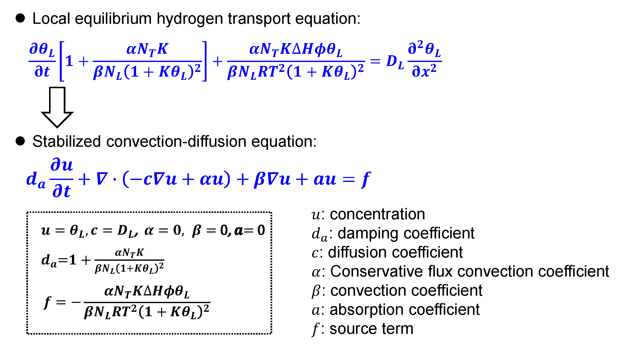
2. Numerical Model
3. Results and Discussion
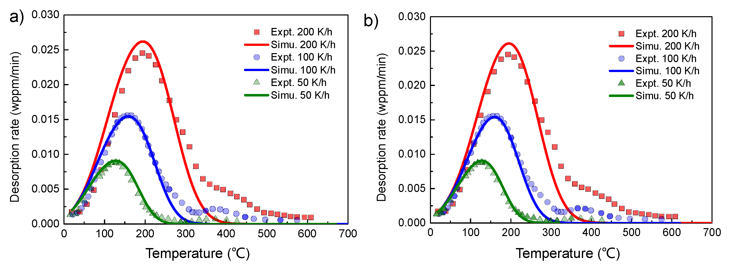
3.1. Validation with Experiment
3.2. Effect of Specimen Geometry
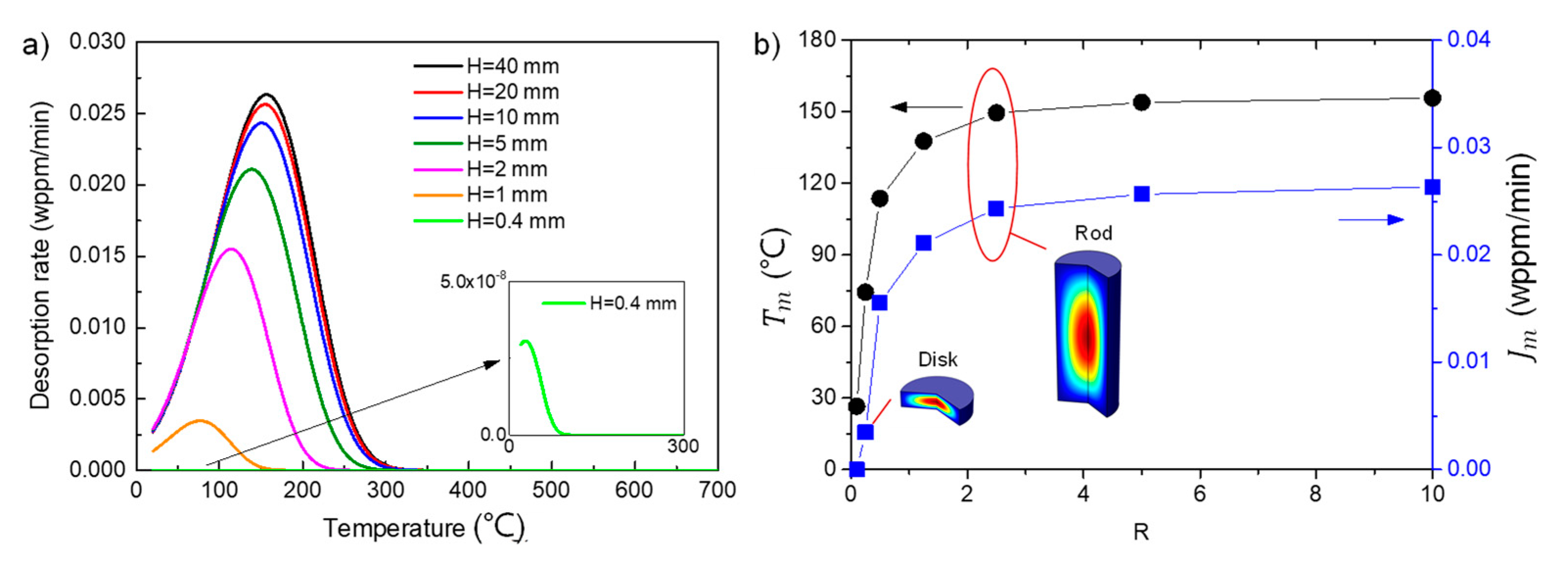
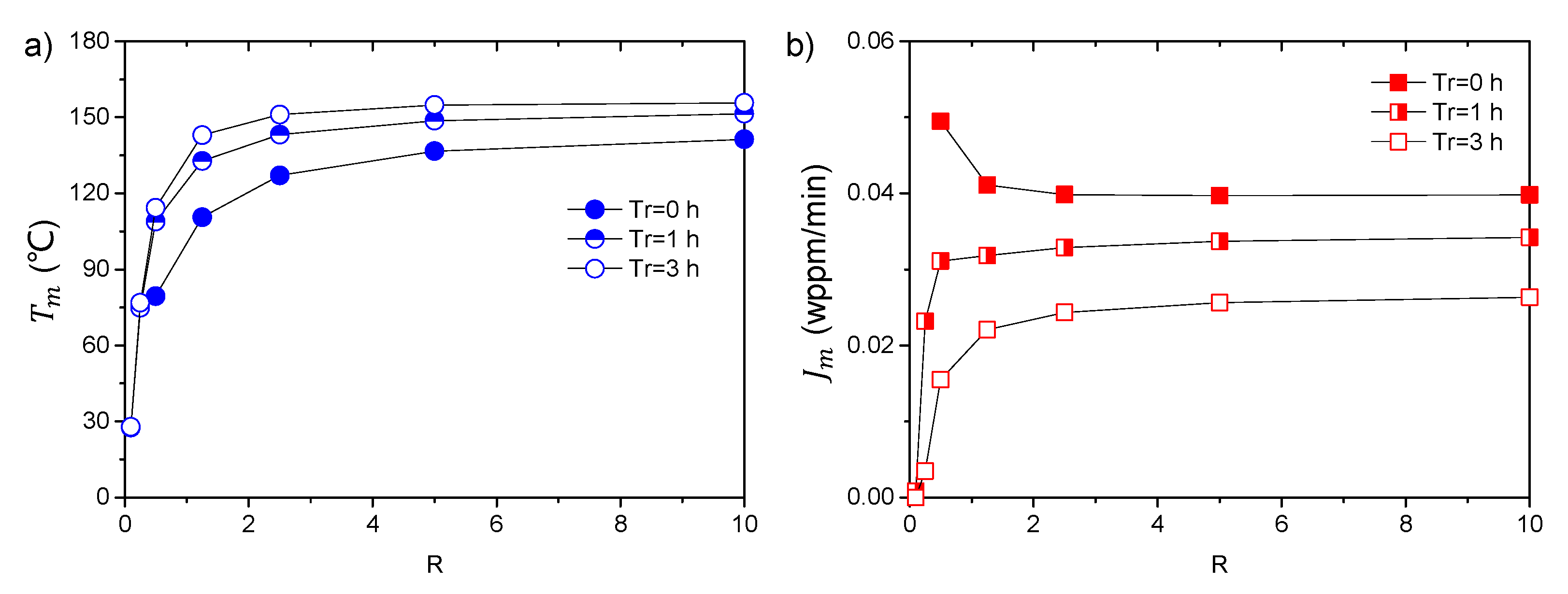
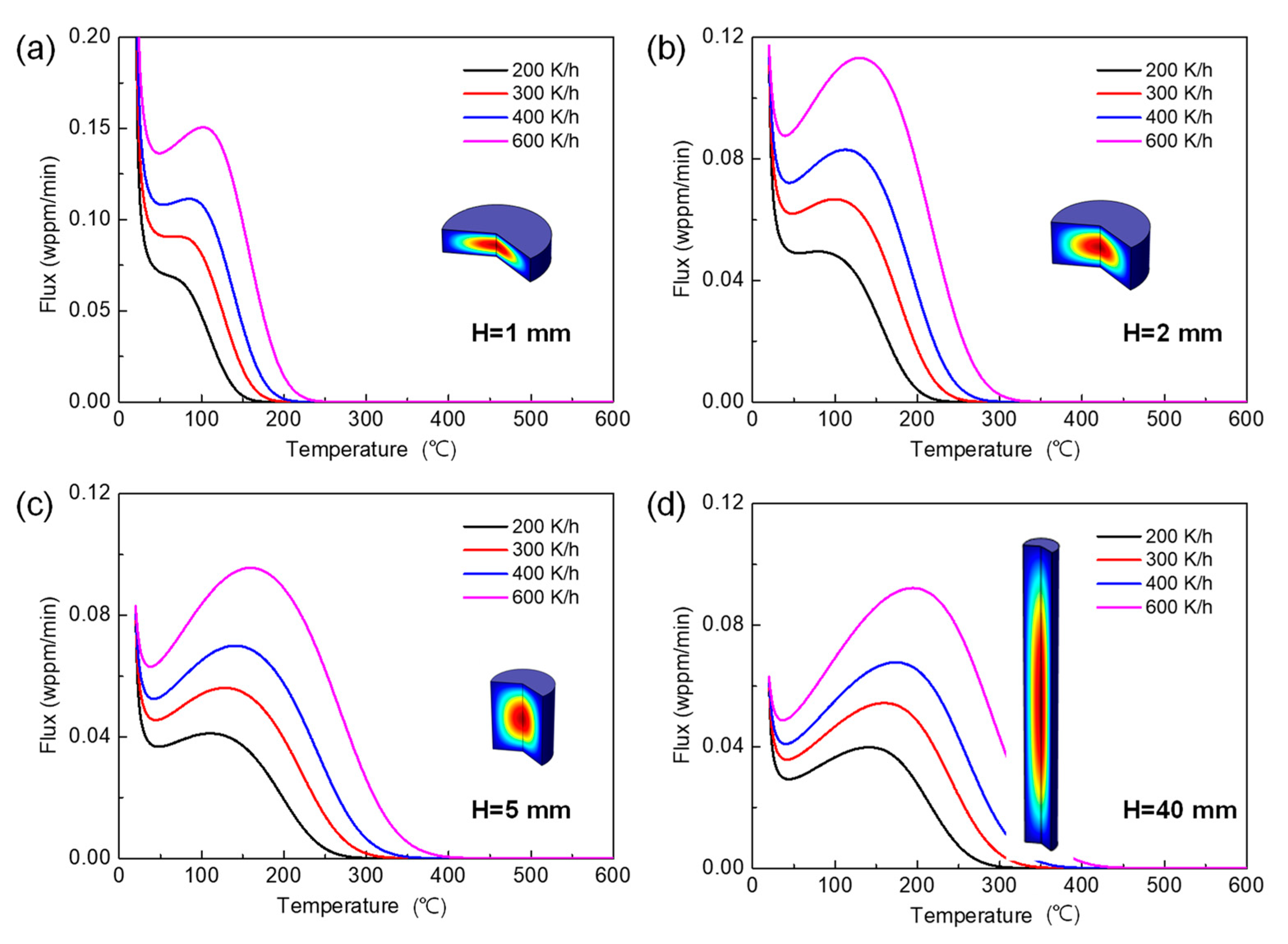
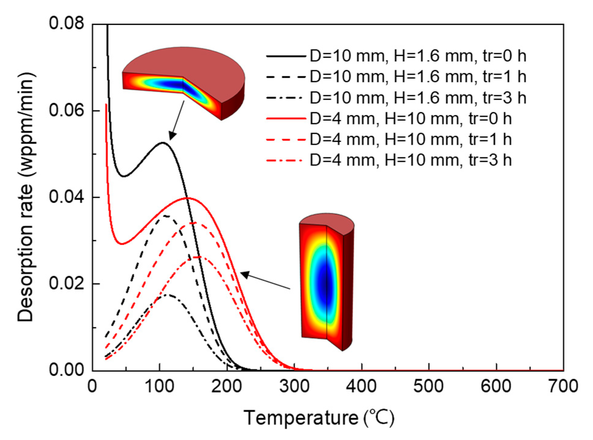
3.2.1. Effect on TDS Curves
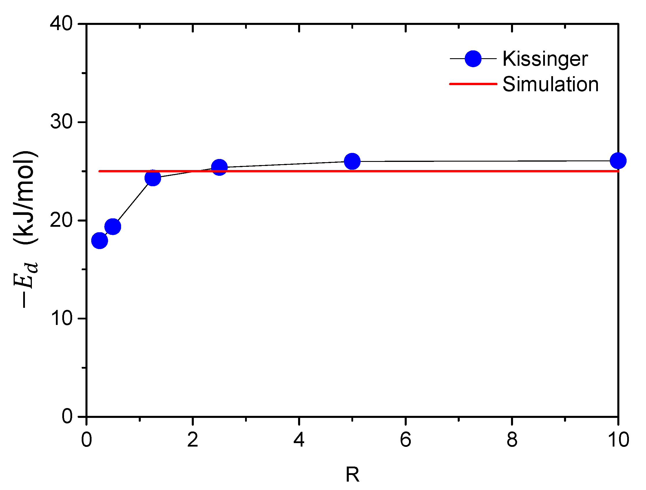
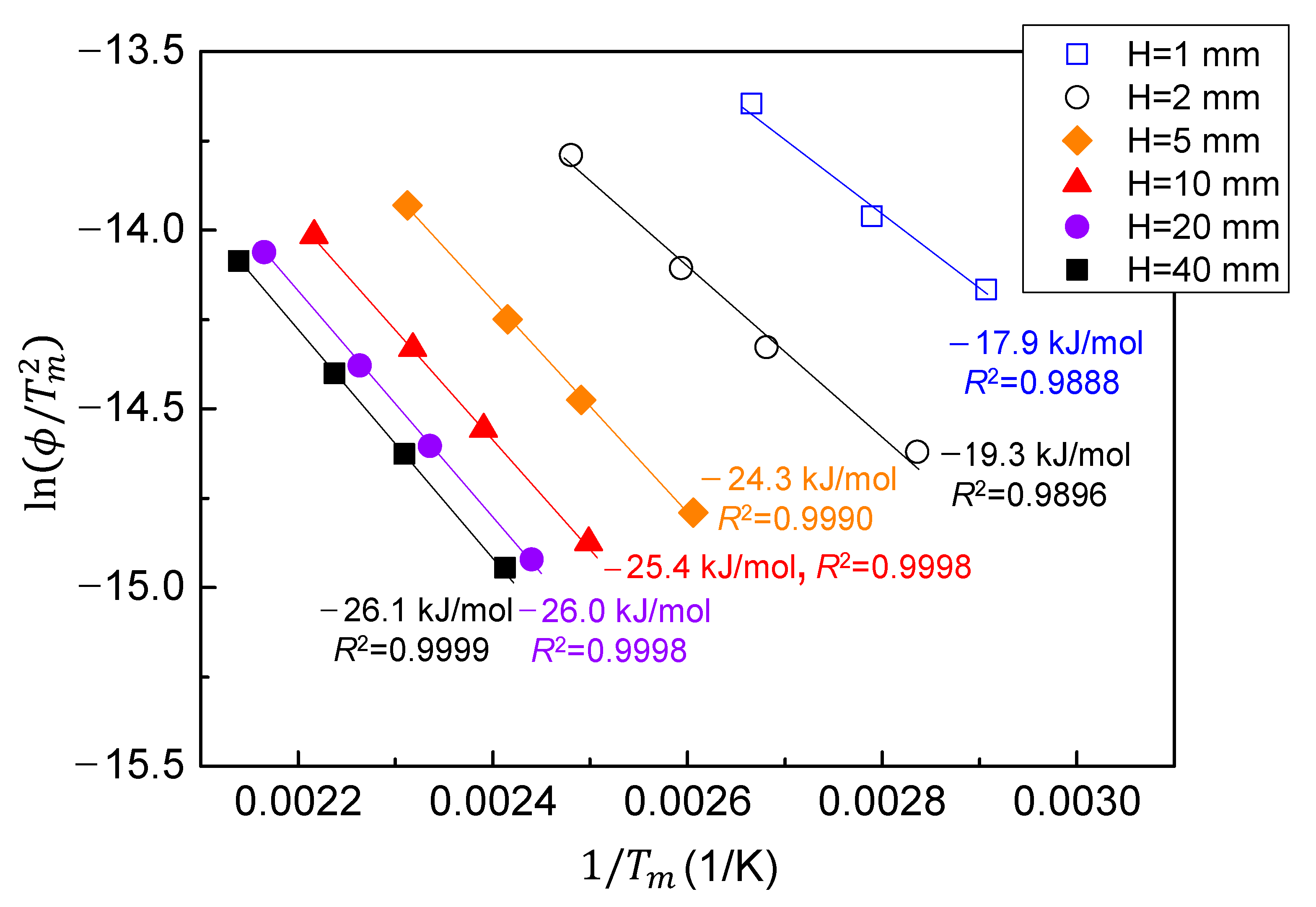
3.2.2. Validity of Kissinger Theory
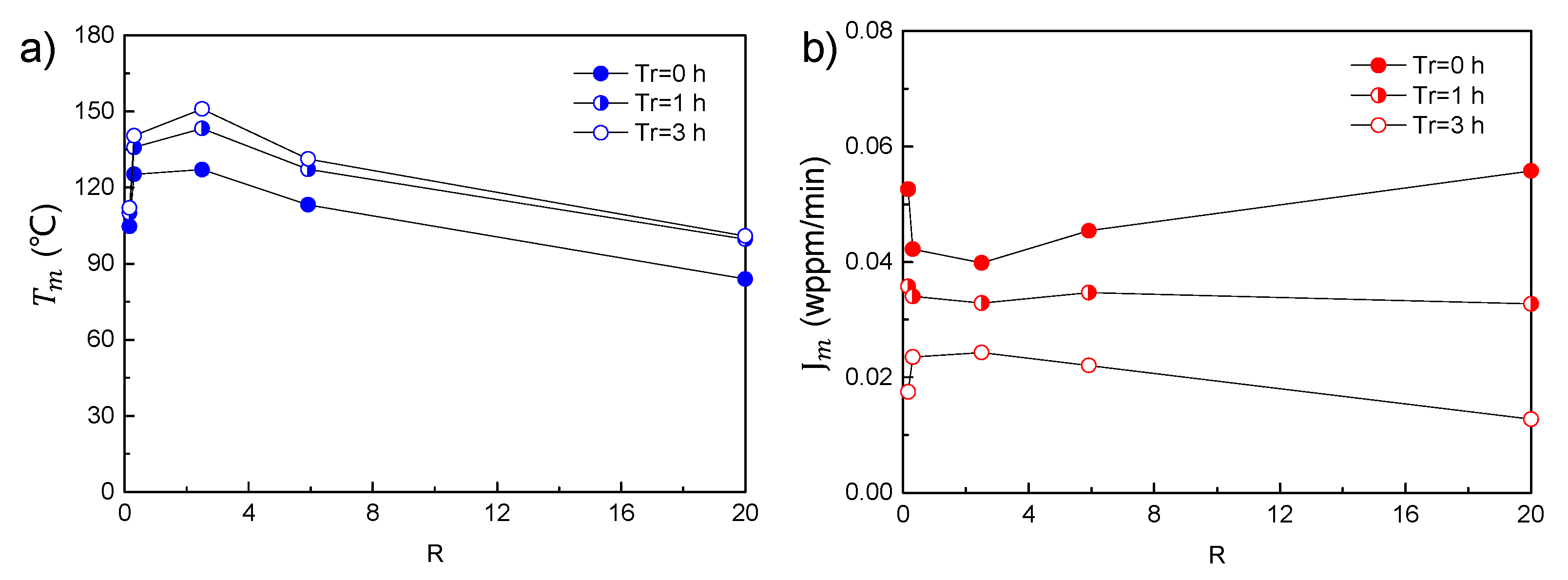
3.2.3. Varied Geometries with Constant Volume
4. Conclusions
Author Contributions
Funding
Institutional Review Board Statement
Informed Consent Statement
Data Availability Statement
Conflicts of Interest
References
- Lee, B.; Karkkainen, R.L. Failure investigation of hydrogen induced cracking of stabilator skin in jet aircraft. Eng. Fail. Anal. 2018, 92, 182–194. [Google Scholar] [CrossRef]
- Sezgin, J.-G.; Bosch, C.; Montouchet, A.; Perrin, G.; Atrens, A.; Wolski, K. Coupled hydrogen and phosphorous induced initiation of internal cracks in a large 18MnNiMo5 component. Eng. Fail. Anal. 2019, 104, 422–438. [Google Scholar] [CrossRef]
- Wasim, M.; Ngo, T.D. Failure analysis of structural steel subjected to long term exposure of hydrogen. Eng. Fail. Anal. 2020, 114, 104606. [Google Scholar] [CrossRef]
- Robertson, I.M.; Sofronis, P.; Nagao, A.; Martin, M.L.; Wang, S.; Gross, D.W.; Nygren, K.E. Hydrogen embrittlement understood. Metall. Mater. Trans. B 2015, 46, 1085–1103. [Google Scholar] [CrossRef]
- Krom, A.H.M.; Koers, R.W.J.; Bakker, A. Hydrogen transport near a blunting crack tip. J. Mech. Phys. Solids 1999, 47, 971–992. [Google Scholar] [CrossRef]
- Kissinger, H.E. Reaction kinetics in differential thermal analysis. Anal. Chem. 1957, 29, 1702–1706. [Google Scholar] [CrossRef]
- Choo, W.Y.; Lee, J.Y. Thermal analysis of trapped hydrogen in pure iron. Metall. Trans. A 1982, 13, 135–140. [Google Scholar] [CrossRef]
- Claeys, L.; Cnockaert, V.; Depover, T.; De Graeve, I.; Verbeken, K. Critical assessment of the evaluation of thermal desorption spectroscopy data for duplex stainless steels: A combined experimental and numerical approach. Acta Mater. 2020, 186, 190–198. [Google Scholar] [CrossRef]
- Pérez Escobar, D.; Depover, T.; Wallaert, E.; Duprez, L.; Verhaege, M.; Verbeken, K. Thermal desorption spectroscopy study of the interaction between hydrogen and different microstructural constituents in lab cast Fe–C alloys. Corros. Sci. 2012, 65, 199–208. [Google Scholar] [CrossRef]
- Wang, M.; Akiyama, E.; Tsuzaki, K. Effect of hydrogen on the fracture behavior of high strength steel during slow strain rate test. Corros. Sci. 2007, 49, 4081–4097. [Google Scholar] [CrossRef]
- Oriani, R.A. The diffusion and trapping of hydrogen in steel. Acta Metall. 1970, 18, 147–157. [Google Scholar] [CrossRef]
- McNabb, A.; Foster, P.K. A new analysis of the diffusion of hydrogen in iron and ferritic steels. Trans. Metall. Soc. AIME 1962, 227, 618–627. [Google Scholar]
- Raina, A.; Deshpande, V.S.; Fleck, N.A. Analysis of thermal desorption of hydrogen in metallic alloys. Acta Mater. 2018, 144, 777–785. [Google Scholar] [CrossRef]
- Tal-Gutelmacher, E.; Eliezer, D.; Abramov, E. Thermal desorption spectroscopy (TDS)—application in quantitative study of hydrogen evolution and trapping in crystalline and non-crystalline materials. Mater. Sci. Eng. A 2007, 445, 625–631. [Google Scholar] [CrossRef]
- Raina, A.; Deshpande, V.; Fleck, N. Analysis of electro-permeation of hydrogen in metallic alloys. Philos. Trans. Soc. A 2017, 375, 20160409. [Google Scholar] [CrossRef] [PubMed]
- Kirchheim, R. Bulk diffusion-controlled thermal desorption spectroscopy with examples for hydrogen in iron. Metall. Mater. Trans. A. 2016, 47, 672–696. [Google Scholar] [CrossRef]
- Wang, Y.F. Effect of initial hydrogen distribution on the parameter extraction of the thermal desorption spectra: A finite element study. Int. J. Hydrog. Energy 2020, 45, 23754–23764. [Google Scholar] [CrossRef]
- Wei, F.-G.; Enomoto, M.; Tsuzaki, K. Applicability of the Kissinger’s formula and comparison with the McNabb–Foster model in simulation of thermal desorption spectrum. Comp. Mater. Sci. 2012, 51, 322–330. [Google Scholar] [CrossRef]
- Pérez Escobar, D.; Duprez, L.; Atrens, A.; Verbeken, K. Influence of experimental parameters on thermal desorption spectroscopy measurements during evaluation of hydrogen trapping. J. Nucl. Mater. 2014, 450, 32–41. [Google Scholar] [CrossRef]
- Song, E.J.; Suh, D.W.; Bhadeshia, H.K.D.H. Theory for hydrogen desorption in ferritic steel. Comp. Mater. Sci. 2013, 79, 36–44. [Google Scholar] [CrossRef]
- Wang, Y.F.; Hu, S.Y.; Li, Y.; Cheng, G.X. Improved hydrogen embrittlement resistance after quenching–tempering treatment for a Cr-Mo-V high strength steel. Int. J. Hydrog. Energy 2019, 44, 29017–29026. [Google Scholar] [CrossRef]
- Novak, P.; Yuan, R.; Somerday, B.P.; Sofronis, P.; Ritchie, R.O. A statistical, physical-based, micro-mechanical model of hydrogen-induced intergranular fracture in steel. J. Mech. Phys. Solids 2010, 58, 206–226. [Google Scholar] [CrossRef]
- Polyanskiy, V.A.; Belyaev, A.K.; Chevrychkina, A.A.; Varshavchik, E.A.; Yakovlev, Y. Impact of skin effect of hydrogen charging on the Choo-Lee plot for cylindrical samples. Int. J. Hydrog. Energy 2020, 46, 6979–6991. [Google Scholar] [CrossRef]
- Castro, F.J.; Meyer, G. Thermal desorption spectroscopy (TDS) method for hydrogen desorption characterization (I): Theoretical aspects. J. Alloys Compd. 2002, 330–332, 59–63. [Google Scholar] [CrossRef]
- COMSOL AB. COMSOL Multiphysics: Quick Start and Quick Reference; COMSOL AB: Burlington, VT, USA, 2007. [Google Scholar]
- Turnbull, A.; Hutchings, R.B.; Ferriss, D.H. Modelling of thermal desorption of hydrogen from metals. Mater. Sci. Eng. A 1997, 238, 317–328. [Google Scholar] [CrossRef]


| H, mm | 1 | 2 | 5 | 10 | 20 | 40 |
|---|---|---|---|---|---|---|
| A * | −2155.2 | −2327.2 | −2925.0 | −3053.2 | −3127.1 | −3134.7 |
| B * | −7.9 | −8.0 | −7.2 | −7.2 | −7.3 | −7.4 |
| R2 | 0.9888 | 0.9896 | 0.9990 | 0.9998 | 0.9998 | 0.9999 |
| Ed, kJ/mol | −17.9 | −19.3 | −24.3 | −25.4 | −26.0 | −26.1 |
| Error, % | −28.4 | −22.8 | −2.8 | 1.6 | 4 | 4.4 |
Publisher’s Note: MDPI stays neutral with regard to jurisdictional claims in published maps and institutional affiliations. |
© 2021 by the authors. Licensee MDPI, Basel, Switzerland. This article is an open access article distributed under the terms and conditions of the Creative Commons Attribution (CC BY) license (http://creativecommons.org/licenses/by/4.0/).
Share and Cite
Wang, Y.; Hu, S.; Cheng, G. Effect of Specimen Geometry on the Thermal Desorption Spectroscopy Evaluated by Two-Dimensional Diffusion-Trapping Coupled Model. Materials 2021, 14, 1374. https://doi.org/10.3390/ma14061374
Wang Y, Hu S, Cheng G. Effect of Specimen Geometry on the Thermal Desorption Spectroscopy Evaluated by Two-Dimensional Diffusion-Trapping Coupled Model. Materials. 2021; 14(6):1374. https://doi.org/10.3390/ma14061374
Chicago/Turabian StyleWang, Yafei, Songyan Hu, and Guangxu Cheng. 2021. "Effect of Specimen Geometry on the Thermal Desorption Spectroscopy Evaluated by Two-Dimensional Diffusion-Trapping Coupled Model" Materials 14, no. 6: 1374. https://doi.org/10.3390/ma14061374
APA StyleWang, Y., Hu, S., & Cheng, G. (2021). Effect of Specimen Geometry on the Thermal Desorption Spectroscopy Evaluated by Two-Dimensional Diffusion-Trapping Coupled Model. Materials, 14(6), 1374. https://doi.org/10.3390/ma14061374