
Buckling Resistance of Two-Segment Stepped Steel Columns


Abstract
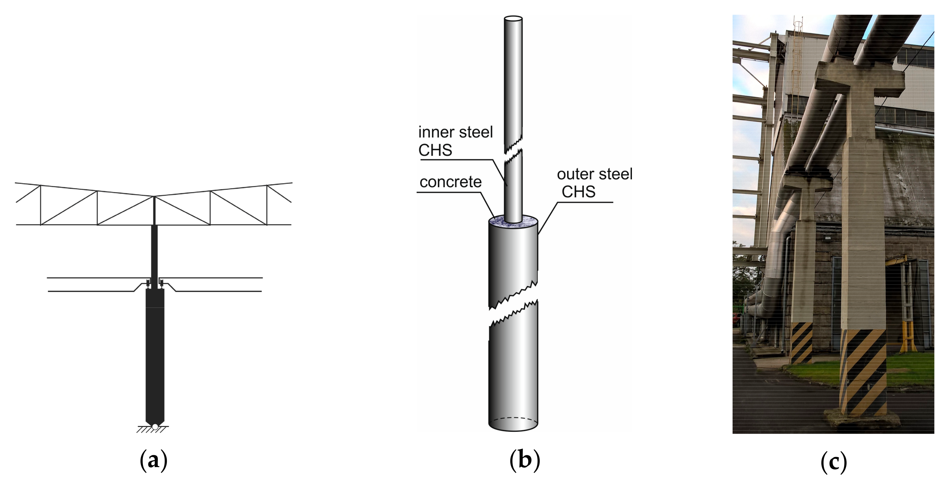
:1. Introduction
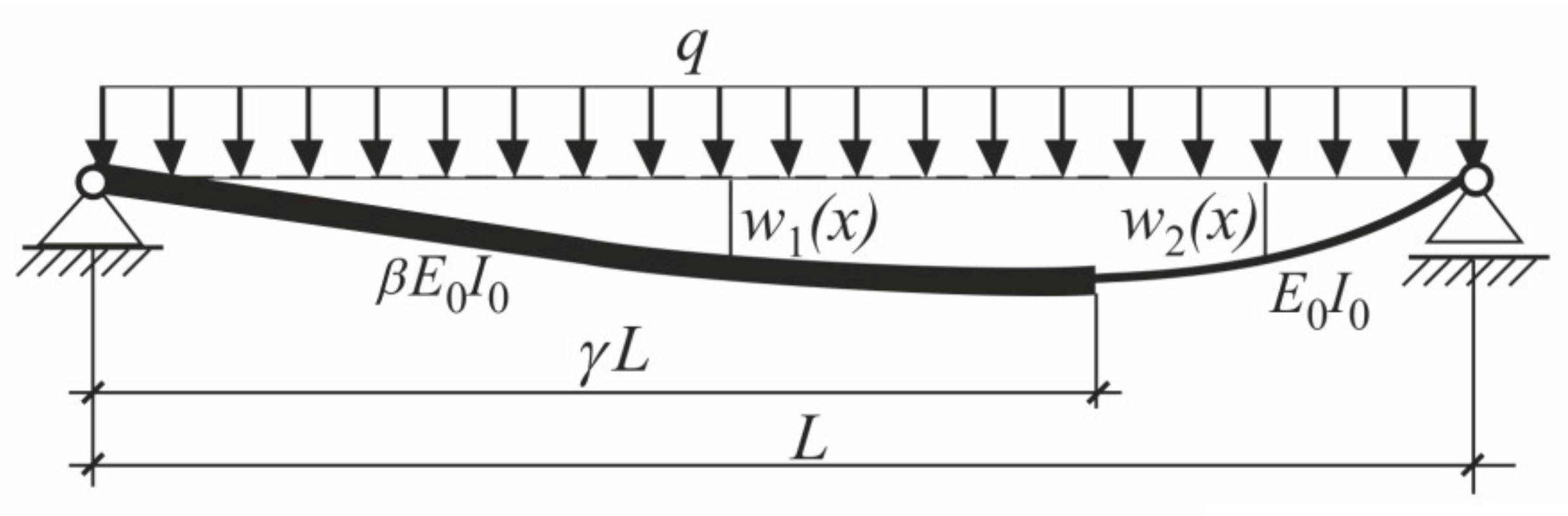
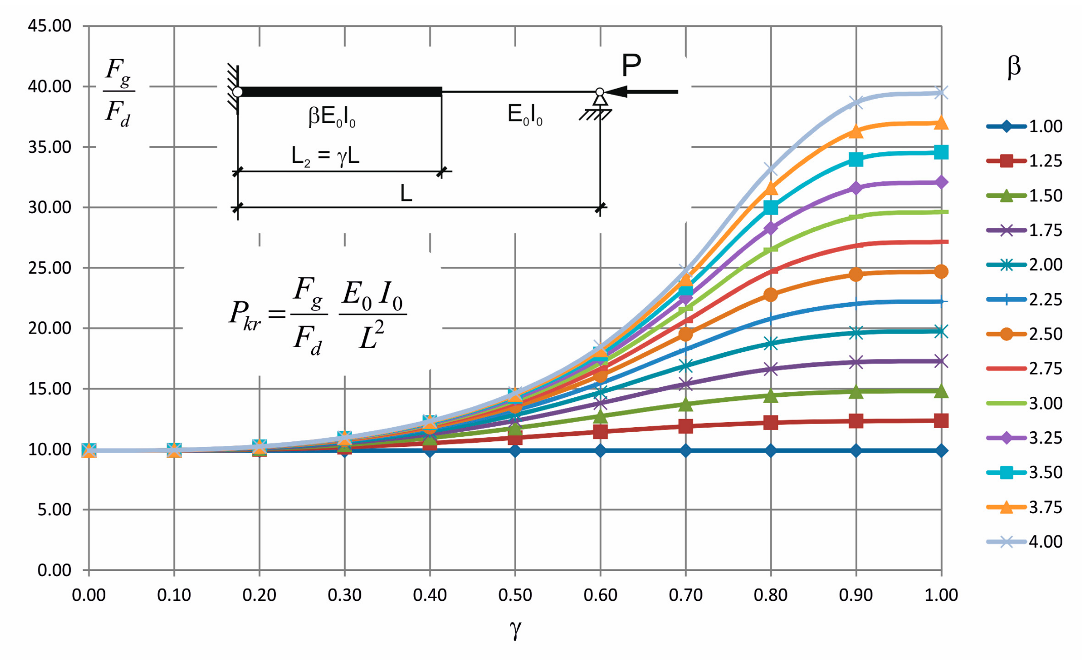
2. Determination of Critical Forces
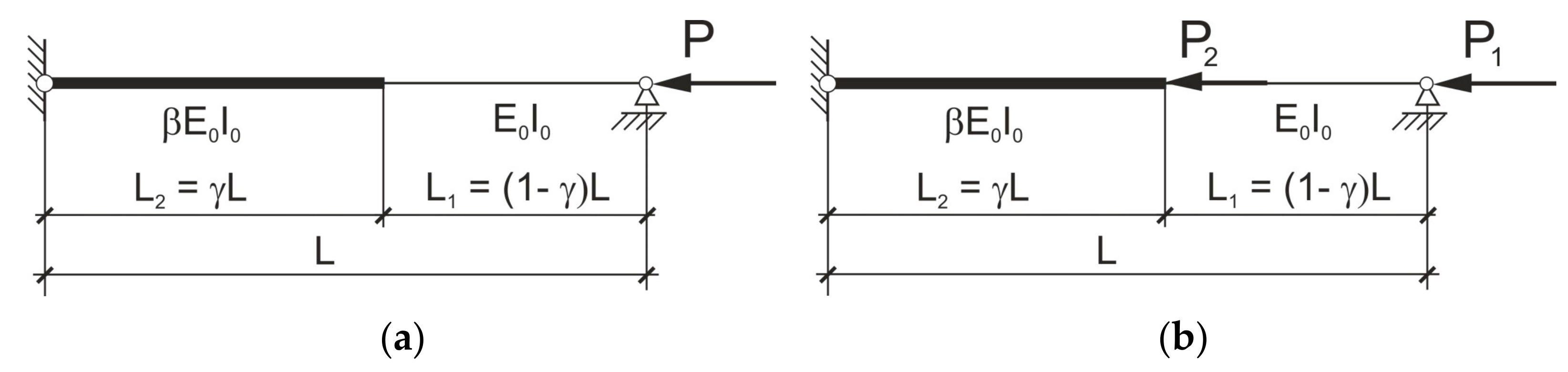
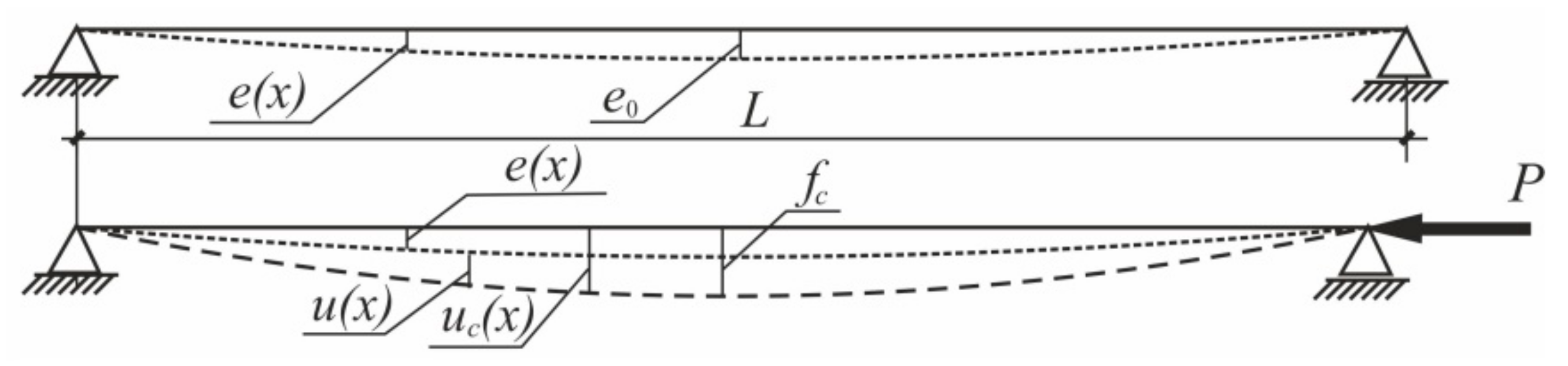
2.1. The Column Loaded by a Force Applied at the End
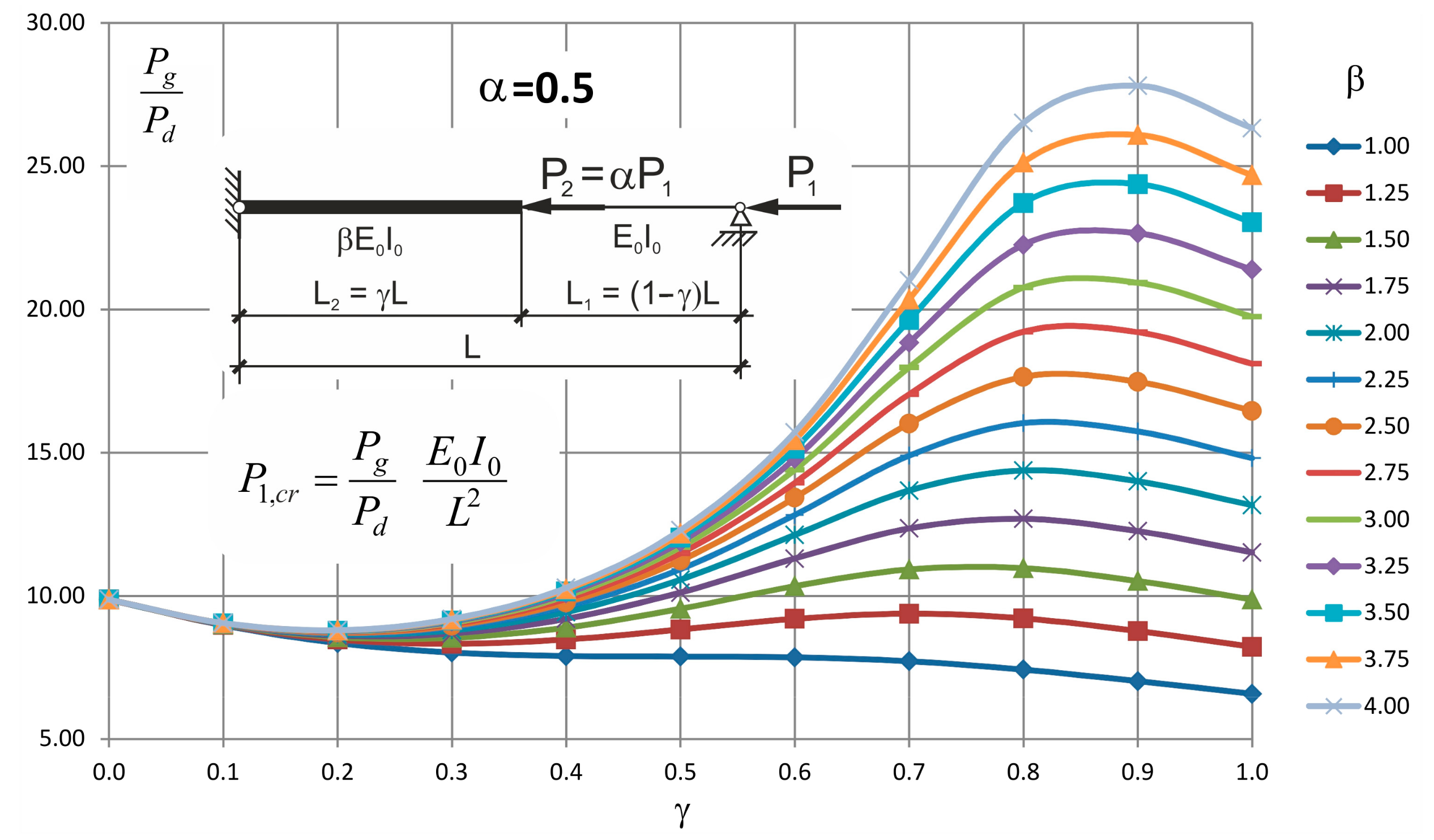
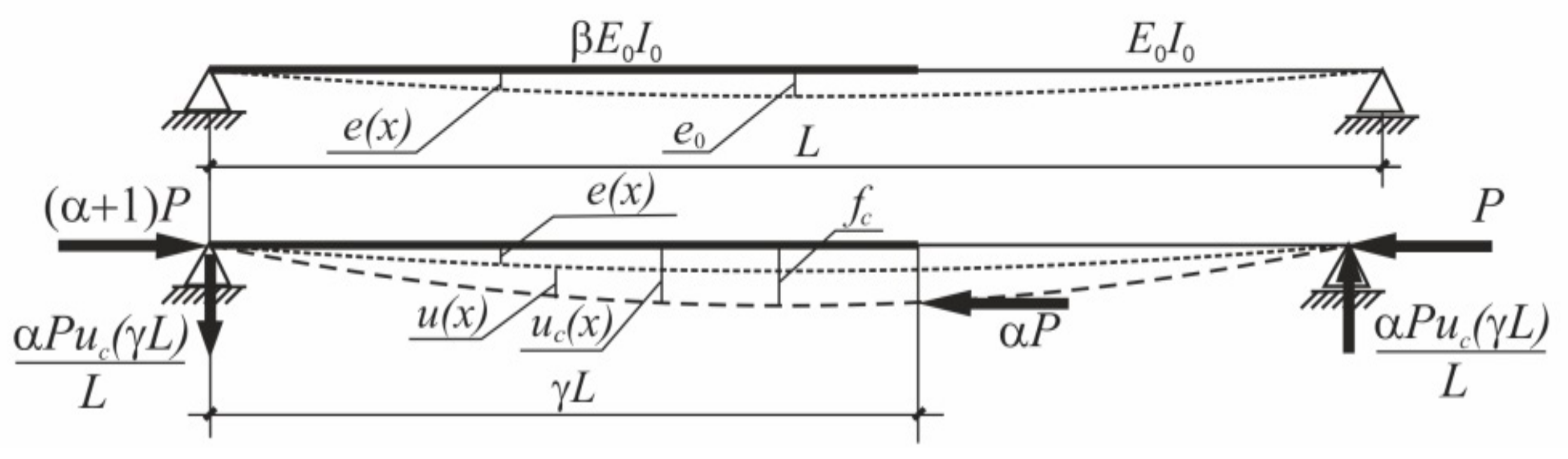
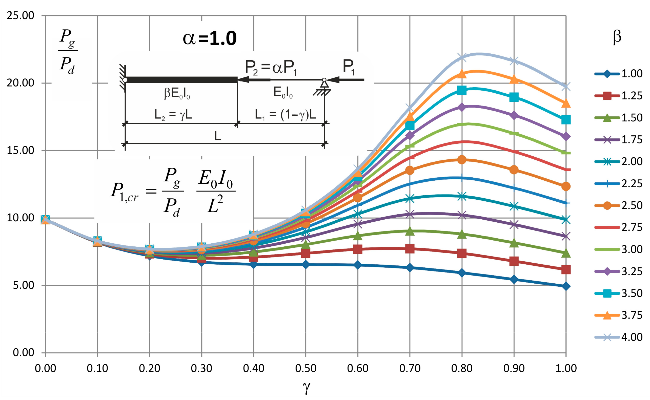
2.2. The Column with Additional Force Acting at the Column’s Span
3. The compressive Resistance of Stepped Steel Columns
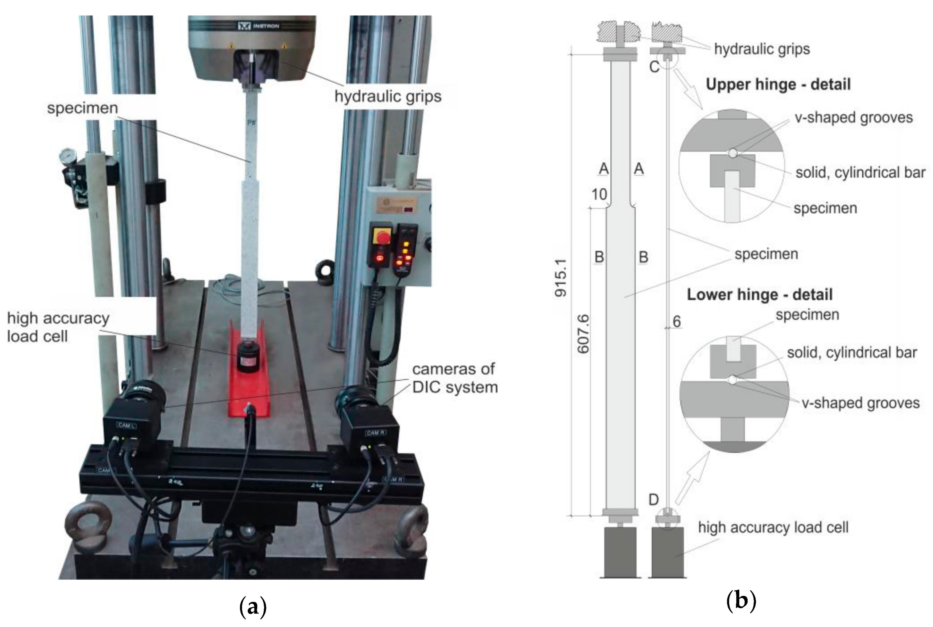
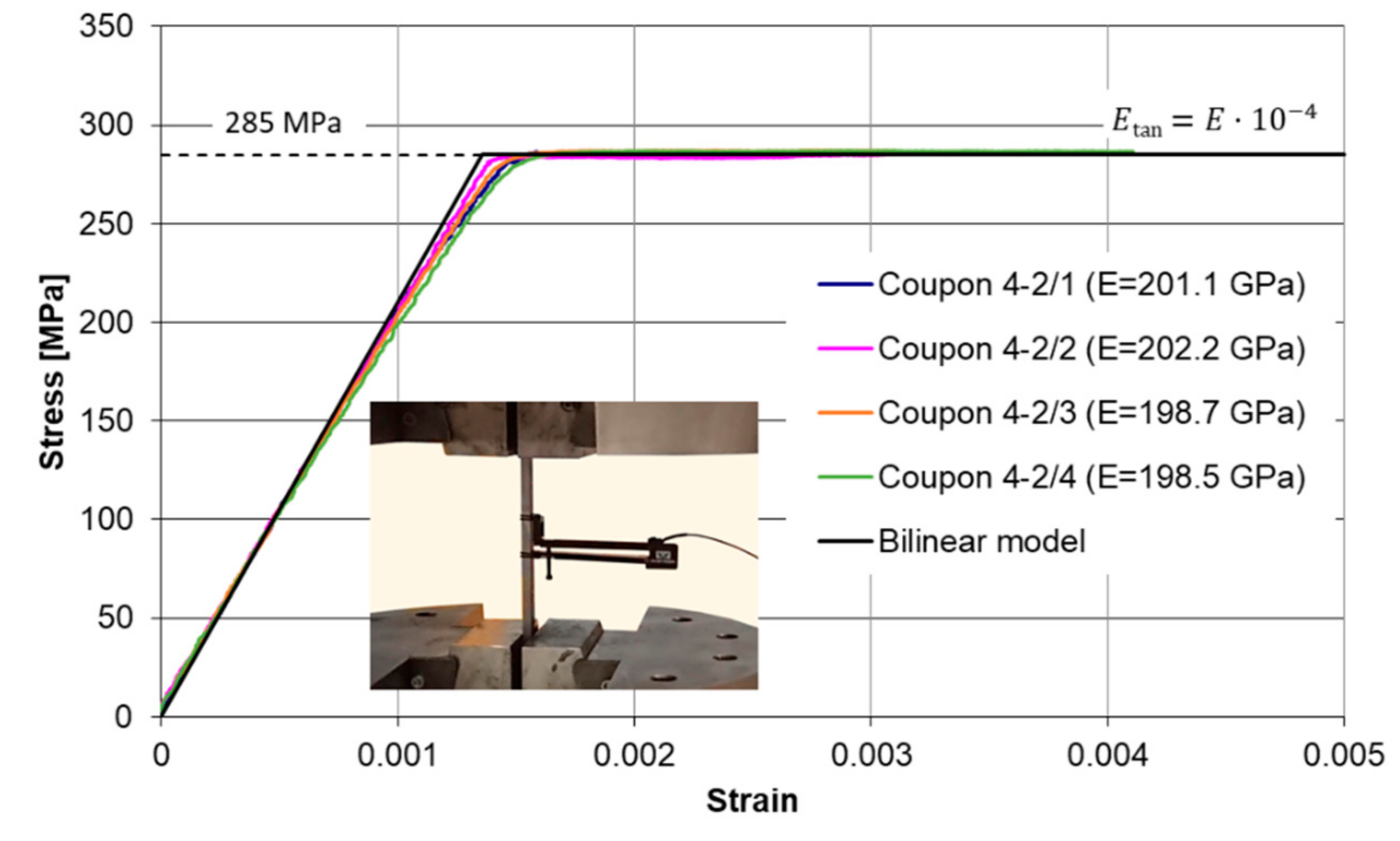
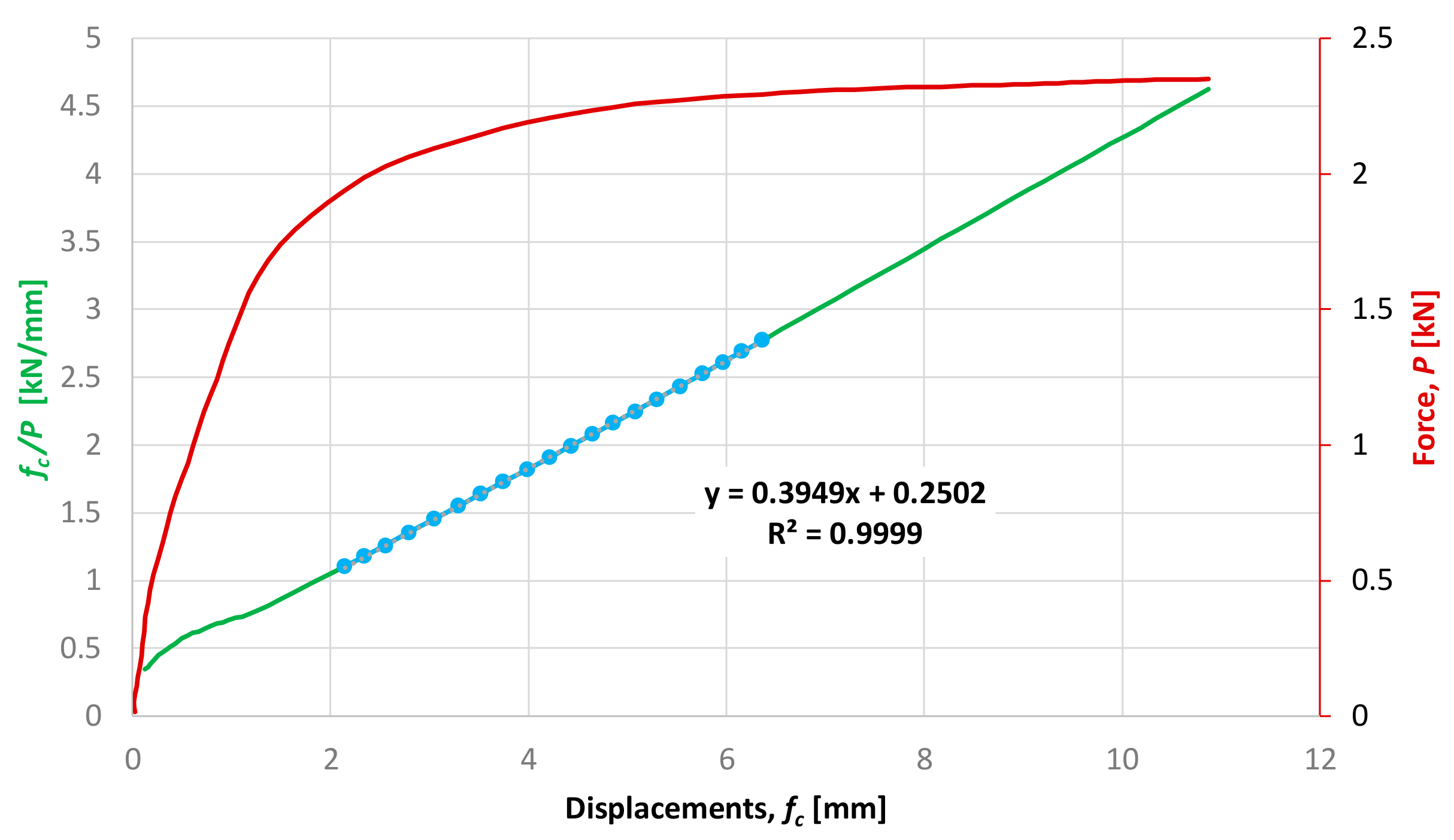
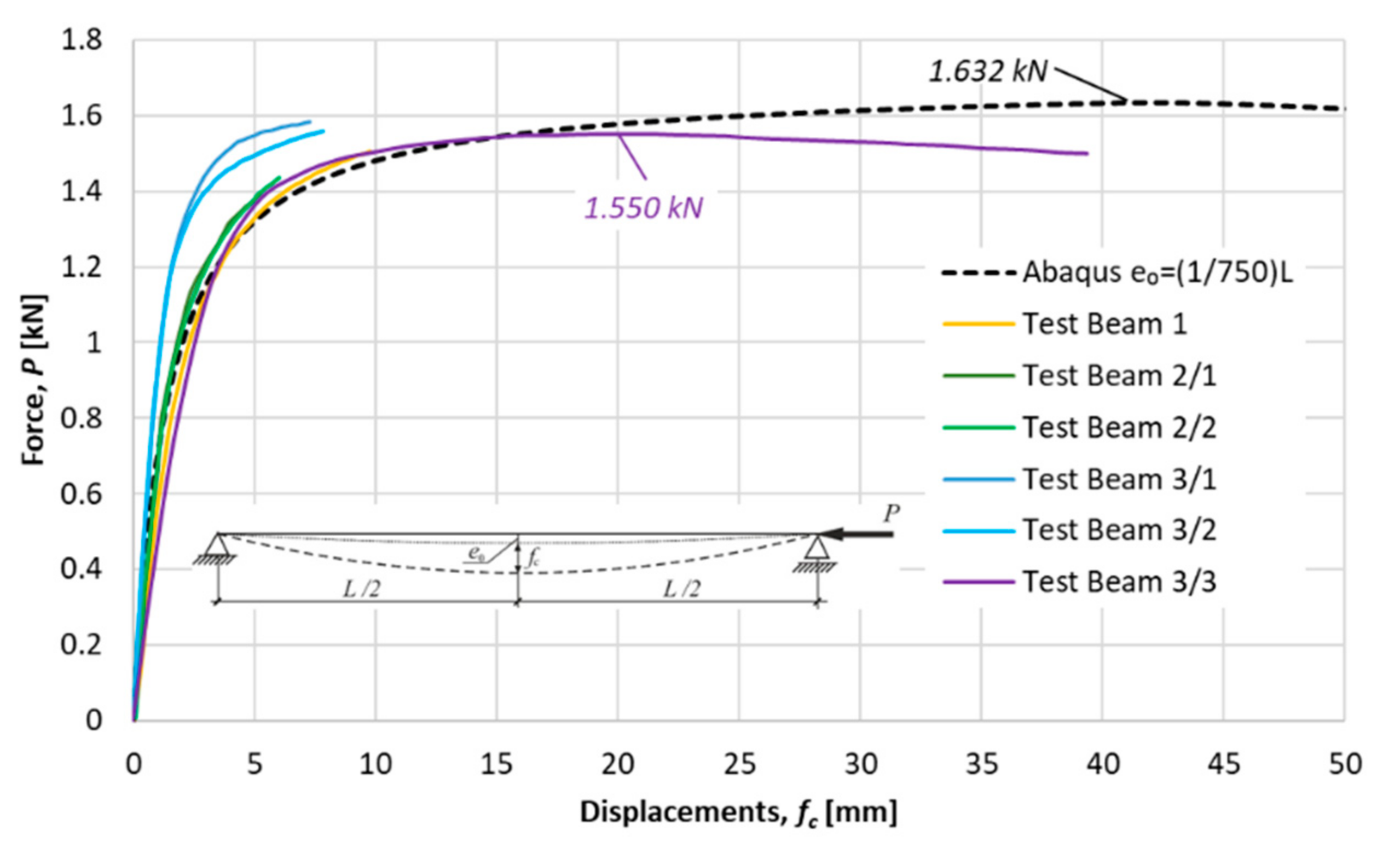
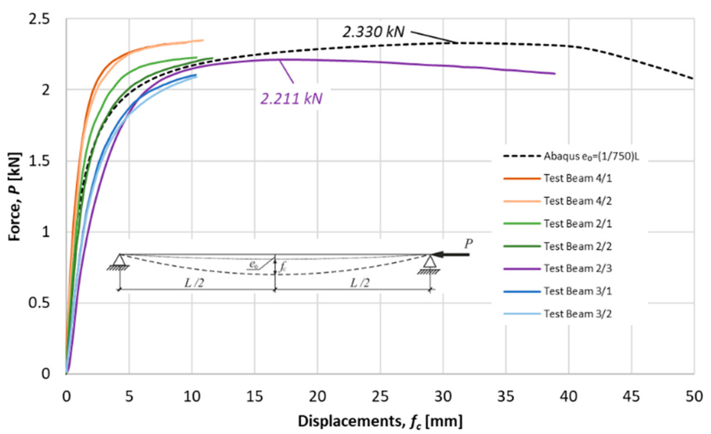
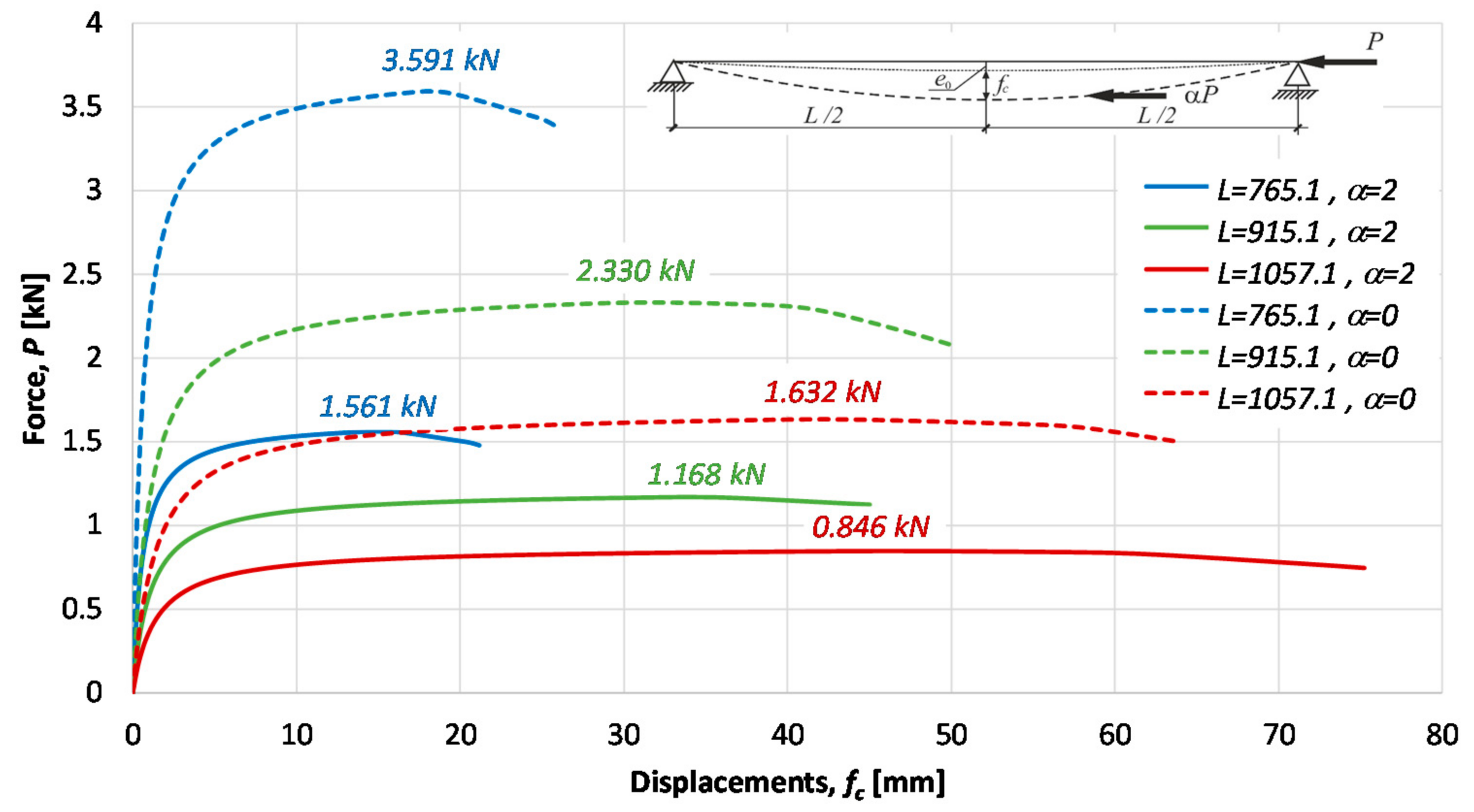
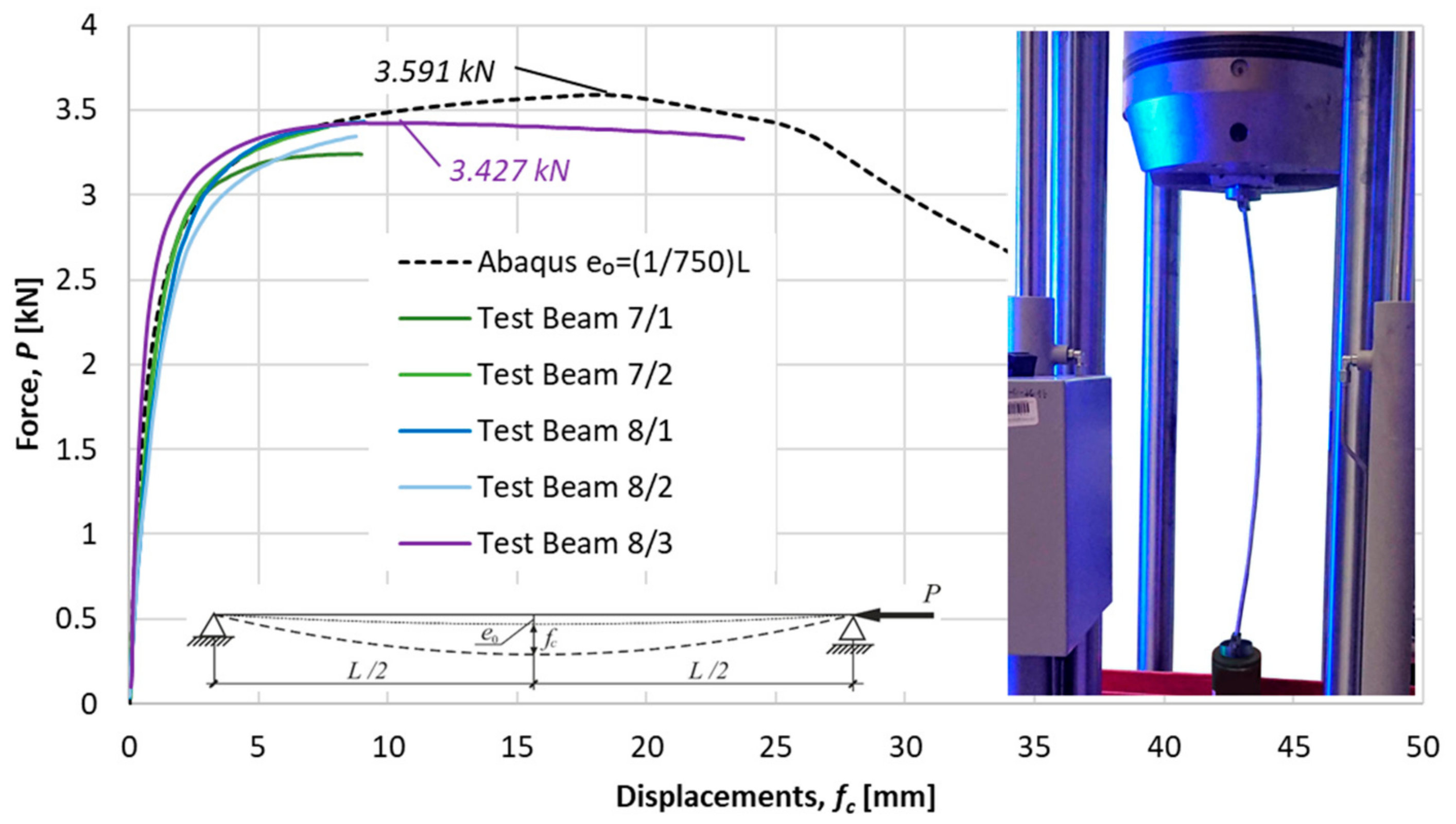
4. Experimental Tests and Numerical Simulations
5. Concluding Remarks
Author Contributions
Funding
Institutional Review Board Statement
Informed Consent Statement
Conflicts of Interest
References
- Timoshenko, S.P.; Gere, J.M. Theory of Elastic Stability, 2nd ed.; McGraw-Hill: New York, NY, USA, 1961. [Google Scholar]
- Volmir, A.S. Stability of Deformable Systems; Nauka: Moscow, Russia, 1967. (In Russian) [Google Scholar]
- Harvey, J.W. Buckling Loads for Stepped Columns. ASCE Proc. ASCE J. Struct. Div. 1964, 90, 201. [Google Scholar] [CrossRef]
- Dalal, S.T. Some Non-Conventional Cases of Column Design. AISC Eng. J. 1969, 6, 28–39. [Google Scholar]
- Anderson, J.P.; Woodward, J.H. Calculation of Effective Lengths and Effective Slenderness Ratios of Stepped Columns. Eng. J. Am. Inst. Steel Constr. 1972, 9, 157–166. [Google Scholar]
- Agrawal, K.M.; Stafiej, A.P. Calculation of effective lengths of stepped columns. Eng. J. Am. Inst. Steel Constr. 1980, 17, 96–105. [Google Scholar]
- Fraser, D.J. The In-Plane Stability of a Frame Containing Pin-Based Stepped Columns. Eng. J. Am. Inst. Steel Constr. 1990, 27, 49–53. [Google Scholar]
- Fraser, D.J.; Bridge, R.Q. Buckling of Stepped Crane Columns. J. Constr. Steel Res. 1990, 16, 23–28. [Google Scholar] [CrossRef]
- Vasquez, J.; Riddell, R. A Simple Stepped-Column Buckling Model and Computer Algorithm. Eng. J. Am. Inst. Steel Constr. 2011, 48, 19–30. [Google Scholar]
- Pinarbasi, S.; Okay, F.; Akpinar, E.; Erdogan, H. Stability Analysis of Two-Segment Stepped Columns with Different End Conditions and Internal Axial Loads. Math. Probl. Eng. 2013, 1–9. [Google Scholar] [CrossRef]
- Salama, M. Elastic Buckling of Single-Stepped Columns with End and Intermediate Axial Loads. Comput. Eng. Phys. Modeling 2018, 1, 25–35. [Google Scholar] [CrossRef]
- Toosi, S.; Esfandiari, A.; Rahbar Ranji, A. Buckling Analysis of Tapered Continuous Columns by Using Modified Buckling Mode Shapes. J. Marine. Sci. Appl. 2019, 18, 160–166. [Google Scholar] [CrossRef]
- Tianab, W.; Haoab, J.; Zhong, W. Buckling of stepped columns considering the interaction effect among columns. J. Constr. Steel Res. 2021, 177. [Google Scholar] [CrossRef]
- Przemieniecki, J.S. Theory of Matrix Structural Analysis; McGraw-Hill, Inc.: New York, NY, USA, 1968. [Google Scholar]
- Simão, P.D.; Girão Coelho, A.M.; Bijlaard, F.S.K. Stability design of crane columns in mill buildings. Eng. Struct. 2012, 42, 51–82. [Google Scholar] [CrossRef]
- Simão, P.D.; Girão Coelho, A.M.; Bijlaard, F.S.K. Influence of splices on the buckling of columns. Int. J. Non Linear Mech. 2012, 47, 806–822. [Google Scholar] [CrossRef]
- Marcinowski, J. Wyboczenie słupów o skokowo zmiennej sztywności giętnej [Buckling of columns with suddenly variable bending stiffness]. In Proceedings of the Metal Structures—ZK 2014, Kielce-Suchedniów, Poland, 2–4 July 2014; Press Engineering & Architecture: Kielce, Poland, 2014; pp. 65–68. (In Polish). [Google Scholar]
- Abaqus Documentation—Massachusetts Institute of Technology. Abaqus documentation. Available online: https://abaqus-docs.mit.edu/2017/English/SIMACAEEXCRefMap/simaexc-c-docproc.htm (accessed on 23 January 2021).
- Abaqus Documentation—Massachusetts Institute of Technology. Finite-Strain Shell Element Formulation. Available online: https://abaqus-docs.mit.edu/2017/English/SIMACAETHERefMap/simathe-c-finitestrainshells.htm (accessed on 23 January 2021).
- Rusiński, E. Finite Element Method: COSMOS/M System; WKŁ: Warsaw, Poland, 1994. (In Polish) [Google Scholar]
- COSMOS/M Finite Element Analysis System; Version 2.5; Structural Research and Analysis Corporation: Los Angeles, CA, USA, 1999.
- Barnes, W.D.; Mangelsdorf, C.P. Allowable Axial Stresses in Segmented Columns. Eng. J. Am. Inst. Steel Constr. 1979, 16, 11–17. [Google Scholar]
- Castiglioni, C.A. Stepped Columns: A Simplified Design Method; Fritz Laboratory Reports; Lehigh University: Milano, Italy, 1984; Available online: https://preserve.lehigh.edu/engr-civil-environmental-fritz-lab-reports/1481 (accessed on 23 January 2021).
- Castiglioni, C.A. Stepped columns: A simplified design method. Eng. J. Am. Inst. Steel Constr. 1986, 23, 1–8. [Google Scholar]
- Boissonnade, N.; Jaspart, J.P.; Muzeau, J.P.; Villette, M. Improvement of the interaction formulae for beam columns in Eurocode 3. Comput. Struct. 2002, 80, 2375–2385. [Google Scholar] [CrossRef]
- Maquoi, R.; Boissonnade, N.; Muzeau, J.P.; Jaspart, J.P.; Villette, M. The interaction formulae for beam-columns: A new step of a yet long story. In Proceedings of the 2001 SSRC Annual Technical Session and Meeting, Fort Lauderdale, FL, USA, 9–12 May 2001; pp. 63–88. [Google Scholar]
- Galambos, T.V. Guide to Stability Design Criteria for Metal Structures, 5th ed.; John Wiley & Sons, Inc.: New York, NY, USA, 1998. [Google Scholar]
- Girão Coelho, A.M.; Simão, P.D.; Bijlaard, F.S.K. Stability design criteria for steel column splices. J. Constr. Steel Res. 2010, 66, 1261–1277. [Google Scholar] [CrossRef]
- Girão Coelho, A.M.; Simão, P.D.; Bijlaard, F.S.K. Practical design of stepped columns. In Proceedings of the 12th Nordic Steel Construction Conference, Oslo, Norway, 5–7 September 2012; Norwegian Steel Association, Ed.; pp. 55–66. [Google Scholar]
- Ayrton, W.E.; Perry, J. On struts. Engineer 1886, 62, 464–465. [Google Scholar]
- Wolfram, S. The Mathematica®, 5th ed.; Wolfram Media: Bodenheim, Germany, 2003. [Google Scholar]


| γ | 0.00 | 0.10 | 0.20 | 0.30 | 0.40 | 0.50 | 0.60 | 0.70 | 0.80 | 0.90 | 1.00 | |
|---|---|---|---|---|---|---|---|---|---|---|---|---|
| β | ||||||||||||
| 1.00 | 9.87 | 9.87 | 9.87 | 9.87 | 9.87 | 9.87 | 9.87 | 9.87 | 9.87 | 9.87 | 9.87 | |
| 1.25 | 9.87 | 9.88 | 9.97 | 10.16 | 10.49 | 10.94 | 11.43 | 11.88 | 12.19 | 12.32 | 12.34 | |
| 1.50 | 9.87 | 9.89 | 10.03 | 10.36 | 10.93 | 11.73 | 12.72 | 13.71 | 14.44 | 14.76 | 14.81 | |
| 1.75 | 9.87 | 9.90 | 10.07 | 10.50 | 11.24 | 12.35 | 13.80 | 15.38 | 16.62 | 17.19 | 17.27 | |
| 2.00 | 9.87 | 9.90 | 10.10 | 10.60 | 11.48 | 12.83 | 14.70 | 16.89 | 18.74 | 19.61 | 19.74 | |
| 2.25 | 9.87 | 9.91 | 10.13 | 10.68 | 11.66 | 13.22 | 15.45 | 18.25 | 20.78 | 22.02 | 22.21 | |
| 2.50 | 9.87 | 9.91 | 10.15 | 10.74 | 11.81 | 13.53 | 16.09 | 19.48 | 22.76 | 24.43 | 24.68 | |
| 2.75 | 9.87 | 9.91 | 10.17 | 10.79 | 11.94 | 13.79 | 16.64 | 20.59 | 24.67 | 26.82 | 27.15 | |
| 3.00 | 9.87 | 9.91 | 10.18 | 10.84 | 12.04 | 14.01 | 17.11 | 21.60 | 26.50 | 29.21 | 29.61 | |
| 3.25 | 9.87 | 9.91 | 10.19 | 10.87 | 12.12 | 14.20 | 17.52 | 22.51 | 28.27 | 31.59 | 32.08 | |
| 3.50 | 9.87 | 9.92 | 10.20 | 10.90 | 12.20 | 14.36 | 17.88 | 23.33 | 29.97 | 33.95 | 34.55 | |
| 3.75 | 9.87 | 9.92 | 10.21 | 10.93 | 12.26 | 14.50 | 18.19 | 24.08 | 31.60 | 36.31 | 37.02 | |
| 4.00 | 9.87 | 9.92 | 10.22 | 10.95 | 12.32 | 14.63 | 18.47 | 24.76 | 33.17 | 38.65 | 39.48 | |
| Column’s Case. Length in (mm) | γ = 607.6/L | Value Resulting from Equation (3) | Equation (6) | COSMOS/M | Abaqus | (Average) |
|---|---|---|---|---|---|---|
| L = 1057.1 | 0.575 | 1.687 | 1.686 | 1.686 | 1.684 | 1.532 |
| L = 915.1 | 0.664 | 2.415 | 2.414 | 2.414 | 2.410 | 2.253 |
| L = 765.1 | 0.794 | 3.721 | 3.720 | 3.722 | 3.718 | 3.490 |
| β | 0.0 | 0.1 | 0.2 | 0.3 | 0.4 | 0.5 | 0.6 | 0.7 | 0.8 | 0.9 | 1.0 | |
|---|---|---|---|---|---|---|---|---|---|---|---|---|
| γ | ||||||||||||
| 1.00 | 9.87 | 8.97 | 8.35 | 8.02 | 7.90 | 7.88 | 7.86 | 7.72 | 7.43 | 7.02 | 6.58 | |
| 1.25 | 9.87 | 8.99 | 8.48 | 8.33 | 8.48 | 8.82 | 9.20 | 9.38 | 9.21 | 8.77 | 8.23 | |
| 1.50 | 9.87 | 9.01 | 8.56 | 8.54 | 8.89 | 9.55 | 10.34 | 10.92 | 10.97 | 10.52 | 9.87 | |
| 1.75 | 9.87 | 9.02 | 8.61 | 8.69 | 9.20 | 10.11 | 11.30 | 12.35 | 12.69 | 12.26 | 11.52 | |
| 2.00 | 9.87 | 9.02 | 8.66 | 8.80 | 9.43 | 10.57 | 12.12 | 13.68 | 14.38 | 14.00 | 13.16 | |
| 2.25 | 9.87 | 9.03 | 8.69 | 8.89 | 9.62 | 10.93 | 12.82 | 14.89 | 16.03 | 15.74 | 14.81 | |
| 2.50 | 9.87 | 9.03 | 8.71 | 8.96 | 9.77 | 11.23 | 13.43 | 16.01 | 17.64 | 17.47 | 16.45 | |
| 2.75 | 9.87 | 9.04 | 8.74 | 9.01 | 9.89 | 11.48 | 13.94 | 17.03 | 19.22 | 19.20 | 18.10 | |
| 3.00 | 9.87 | 9.04 | 8.75 | 9.06 | 10.00 | 11.70 | 14.39 | 17.97 | 20.75 | 20.93 | 19.74 | |
| 3.25 | 9.87 | 9.04 | 8.77 | 9.10 | 10.08 | 11.88 | 14.79 | 18.83 | 22.25 | 22.65 | 21.39 | |
| 3.50 | 9.87 | 9.05 | 8.78 | 9.14 | 10.16 | 12.04 | 15.13 | 19.62 | 23.71 | 24.37 | 23.03 | |
| 3.75 | 9.87 | 9.05 | 8.79 | 9.17 | 10.22 | 12.17 | 15.44 | 20.34 | 25.12 | 26.09 | 24.68 | |
| 4.00 | 9.87 | 9.05 | 8.80 | 9.19 | 10.28 | 12.29 | 15.71 | 21.01 | 26.50 | 27.80 | 26.32 | |
| β | 0.00 | 0.10 | 0.20 | 0.30 | 0.40 | 0.50 | 0.60 | 0.70 | 0.80 | 0.90 | 1.00 | |
|---|---|---|---|---|---|---|---|---|---|---|---|---|
| γ | ||||||||||||
| 1.00 | 9.87 | 8.18 | 7.20 | 6.73 | 6.56 | 6.55 | 6.51 | 6.31 | 5.93 | 5.44 | 4.94 | |
| 1.25 | 9.87 | 8.21 | 7.33 | 7.03 | 7.10 | 7.38 | 7.68 | 7.71 | 7.38 | 6.80 | 6.17 | |
| 1.50 | 9.87 | 8.23 | 7.42 | 7.23 | 7.48 | 8.03 | 8.68 | 9.04 | 8.80 | 8.15 | 7.40 | |
| 1.75 | 9.87 | 8.25 | 7.48 | 7.38 | 7.77 | 8.55 | 9.55 | 10.28 | 10.21 | 9.51 | 8.64 | |
| 2.00 | 9.87 | 8.26 | 7.53 | 7.49 | 7.99 | 8.96 | 10.29 | 11.44 | 11.60 | 10.86 | 9.87 | |
| 2.25 | 9.87 | 8.26 | 7.57 | 7.58 | 8.16 | 9.30 | 10.93 | 12.52 | 12.97 | 12.21 | 11.10 | |
| 2.50 | 9.87 | 8.27 | 7.60 | 7.65 | 8.31 | 9.58 | 11.49 | 13.52 | 14.31 | 13.56 | 12.34 | |
| 2.75 | 9.87 | 8.27 | 7.62 | 7.71 | 8.43 | 9.82 | 11.97 | 14.45 | 15.64 | 14.91 | 13.57 | |
| 3.00 | 9.87 | 8.28 | 7.64 | 7.76 | 8.53 | 10.02 | 12.39 | 15.32 | 16.94 | 16.26 | 14.81 | |
| 3.25 | 9.87 | 8.28 | 7.66 | 7.80 | 8.61 | 10.19 | 12.76 | 16.11 | 18.21 | 17.61 | 16.04 | |
| 3.50 | 9.87 | 8.29 | 7.67 | 7.84 | 8.68 | 10.34 | 13.09 | 16.85 | 19.46 | 18.95 | 17.27 | |
| 3.75 | 9.87 | 8.29 | 7.69 | 7.87 | 8.75 | 10.47 | 13.38 | 17.53 | 20.69 | 20.29 | 18.51 | |
| 4.00 | 9.87 | 8.29 | 7.70 | 7.89 | 8.80 | 10.59 | 13.64 | 18.16 | 21.89 | 21.64 | 19.74 | |
| β | 0.0 | 0.1 | 0.2 | 0.3 | 0.4 | 0.5 | 0.6 | 0.7 | 0.8 | 0.9 | 1.0 | |
|---|---|---|---|---|---|---|---|---|---|---|---|---|
| γ | ||||||||||||
| 1.00 | 9.87 | 6.91 | 5.59 | 5.06 | 4.89 | 4.88 | 4.83 | 4.61 | 4.21 | 3.75 | 3.29 | |
| 1.25 | 9.87 | 6.94 | 5.73 | 5.32 | 5.33 | 5.55 | 5.75 | 5.67 | 5.25 | 4.68 | 4.11 | |
| 1.50 | 9.87 | 6.97 | 5.82 | 5.51 | 5.65 | 6.08 | 6.55 | 6.68 | 6.28 | 5.62 | 4.94 | |
| 1.75 | 9.87 | 6.99 | 5.89 | 5.64 | 5.90 | 6.51 | 7.26 | 7.65 | 7.31 | 6.55 | 5.76 | |
| 2.00 | 9.87 | 7.00 | 5.94 | 5.75 | 6.09 | 6.86 | 7.87 | 8.57 | 8.32 | 7.49 | 6.58 | |
| 2.25 | 9.87 | 7.01 | 5.97 | 5.83 | 6.25 | 7.15 | 8.41 | 9.44 | 9.33 | 8.42 | 7.40 | |
| 2.50 | 9.87 | 7.02 | 6.01 | 5.90 | 6.37 | 7.39 | 8.89 | 10.26 | 10.33 | 9.36 | 8.23 | |
| 2.75 | 9.87 | 7.03 | 6.03 | 5.95 | 6.48 | 7.59 | 9.30 | 11.03 | 11.32 | 10.29 | 9.05 | |
| 3.00 | 9.87 | 7.03 | 6.05 | 6.00 | 6.57 | 7.77 | 9.67 | 11.75 | 12.30 | 11.22 | 9.87 | |
| 3.25 | 9.87 | 7.04 | 6.07 | 6.04 | 6.64 | 7.92 | 9.99 | 12.43 | 13.26 | 12.16 | 10.69 | |
| 3.50 | 9.87 | 7.04 | 6.09 | 6.07 | 6.71 | 8.05 | 10.28 | 13.06 | 14.22 | 13.09 | 11.52 | |
| 3.75 | 9.87 | 7.05 | 6.10 | 6.10 | 6.77 | 8.16 | 10.53 | 13.66 | 15.16 | 14.02 | 12.34 | |
| 4.00 | 9.87 | 7.05 | 6.11 | 6.12 | 6.82 | 8.27 | 10.76 | 14.21 | 16.09 | 14.95 | 13.16 | |
| Column’s Case. Length in [mm] | γ = 607.6/L | Value Resulting from Equation (8) | Equation (18) | COSMOS/M | Abaqus |
|---|---|---|---|---|---|
| L = 1057.1 | 0.575 | 0.8727 | 0.8706 | 0.8708 | 0.8699 |
| L = 915.1 | 0.664 | 1.2093 | 1.2026 | 1.2031 | 1.2020 |
| L = 765.1 | 0.794 | 1.6319 | 1.6215 | 1.6226 | 1.6217 |
| Column’s Case. Length in (mm) | γ = 607.6/L | Critical Force Pcr | Abaqus | col.5/col.4 | |
|---|---|---|---|---|---|
| L = 1057.1 | 0.575 | 1.687 | 1.483 | 1.632 | 1.10 |
| L = 915.1 | 0.664 | 2.415 | 2.114 | 2.330 | 1.10 |
| L = 765.1 | 0.794 | 3.721 | 3.257 | 3.591 | 1.10 |
| Column’s Case. Length in (mm) | γ = 607.6/L | Critical Force Pcr | Abaqus | col.5/col.4 | |
|---|---|---|---|---|---|
| L = 1057.1 | 0.575 | 0.8727 | 0.7668 | 0.8460 | 1.10 |
| L = 915.1 | 0.664 | 1.2093 | 1.060 | 1.1681 | 1.10 |
| L = 765.1 | 0.794 | 1.6319 | 1.418 | 1.5613 | 1.10 |
Publisher’s Note: MDPI stays neutral with regard to jurisdictional claims in published maps and institutional affiliations. |
© 2021 by the authors. Licensee MDPI, Basel, Switzerland. This article is an open access article distributed under the terms and conditions of the Creative Commons Attribution (CC BY) license (http://creativecommons.org/licenses/by/4.0/).
Share and Cite
Fliegner, B.; Marcinowski, J.; Sakharov, V. Buckling Resistance of Two-Segment Stepped Steel Columns. Materials 2021, 14, 1046. https://doi.org/10.3390/ma14041046
Fliegner B, Marcinowski J, Sakharov V. Buckling Resistance of Two-Segment Stepped Steel Columns. Materials. 2021; 14(4):1046. https://doi.org/10.3390/ma14041046
Chicago/Turabian StyleFliegner, Bartłomiej, Jakub Marcinowski, and Volodymyr Sakharov. 2021. "Buckling Resistance of Two-Segment Stepped Steel Columns" Materials 14, no. 4: 1046. https://doi.org/10.3390/ma14041046
APA StyleFliegner, B., Marcinowski, J., & Sakharov, V. (2021). Buckling Resistance of Two-Segment Stepped Steel Columns. Materials, 14(4), 1046. https://doi.org/10.3390/ma14041046