
Nonlinear Dynamic Modeling and Analysis of an L-Shaped Multi-Beam Jointed Structure with Tip Mass


Abstract
:1. Introduction
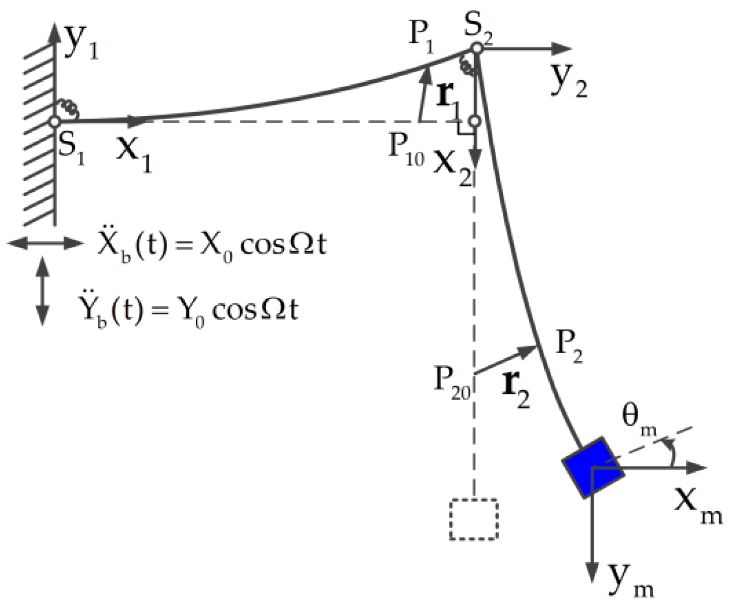
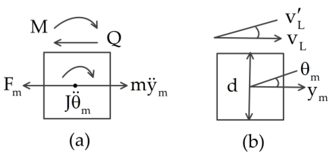
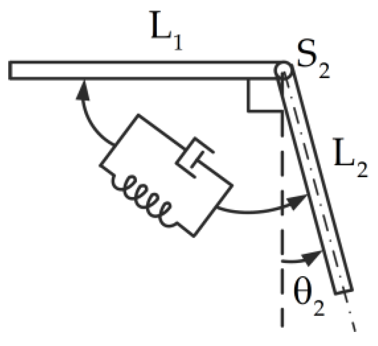
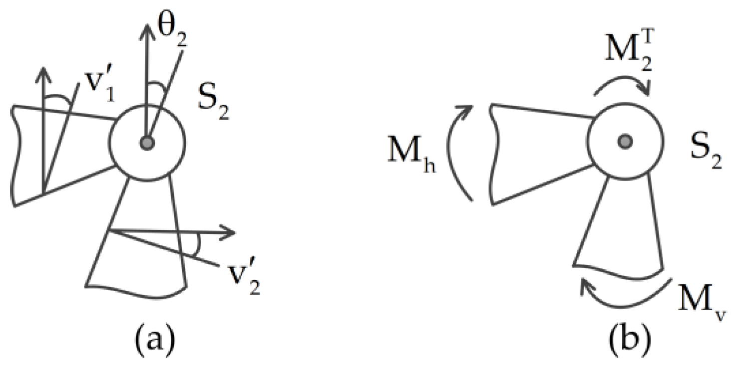
2. Dynamical Model
2.1. Governing Equations of Motion
2.2. Determination of Natural Frequencies and Global Mode Shapes
2.3. Orthogonality of the Global Mode Shapes
2.4. Dynamic Model with Multi-DOF
3. Results and Discussion
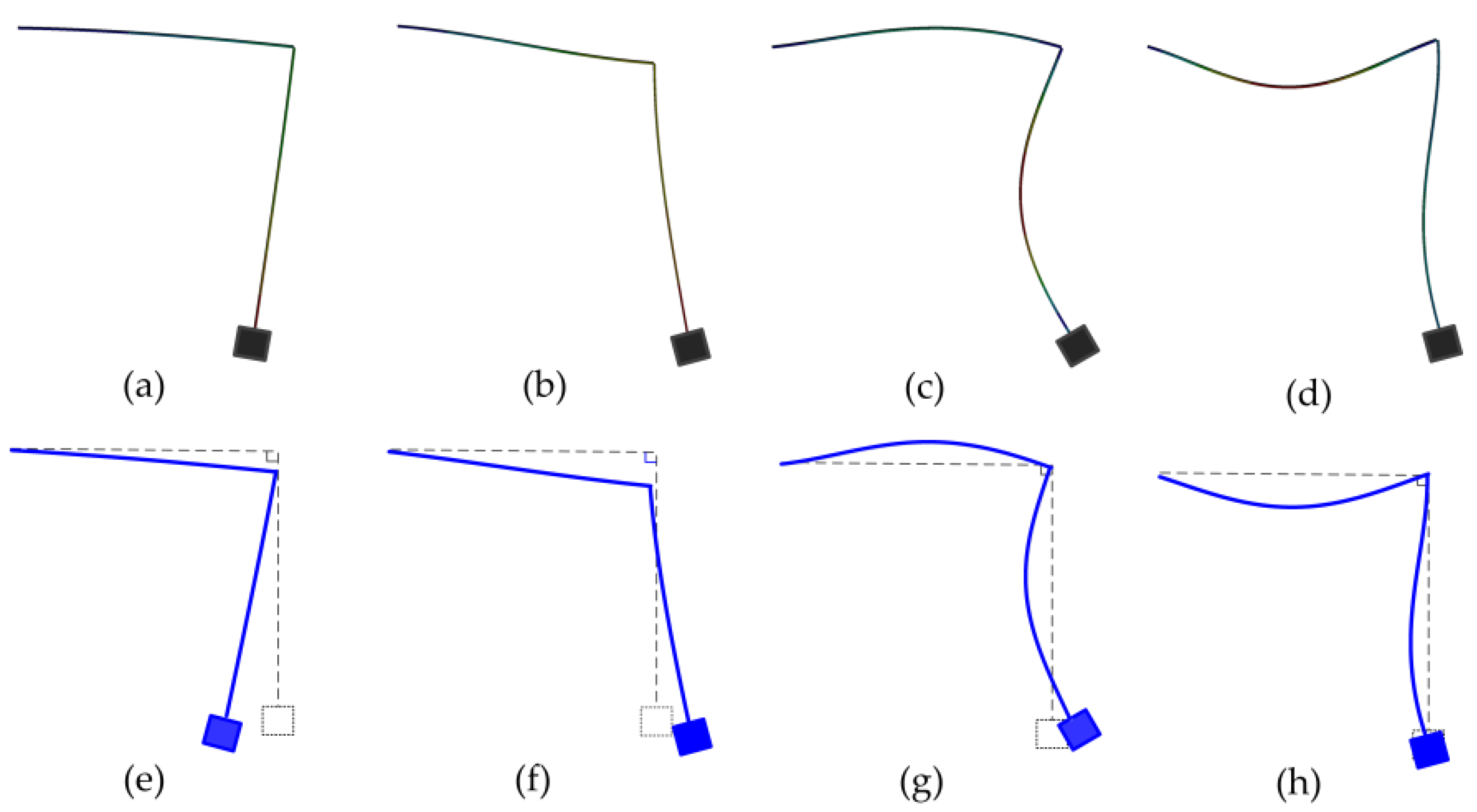
3.1. Mode Analysis
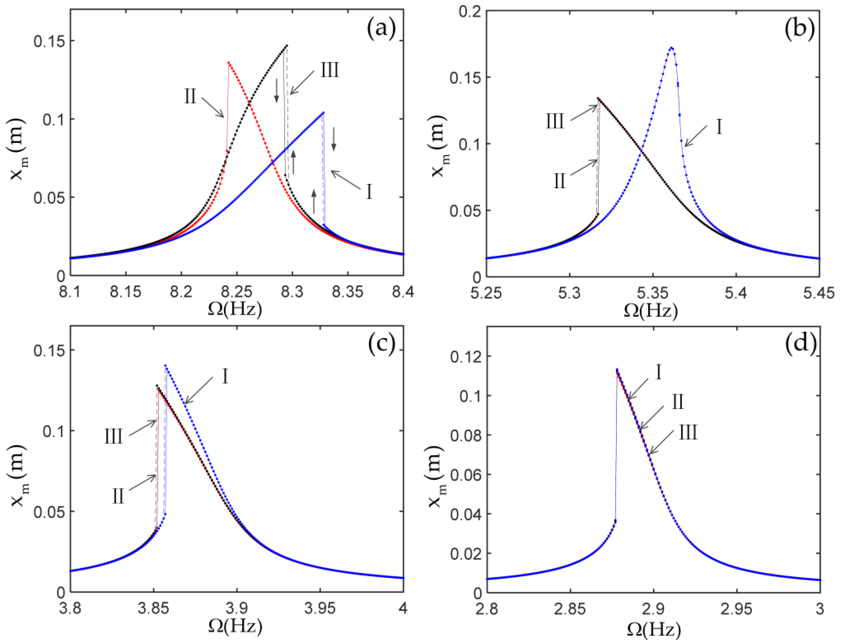
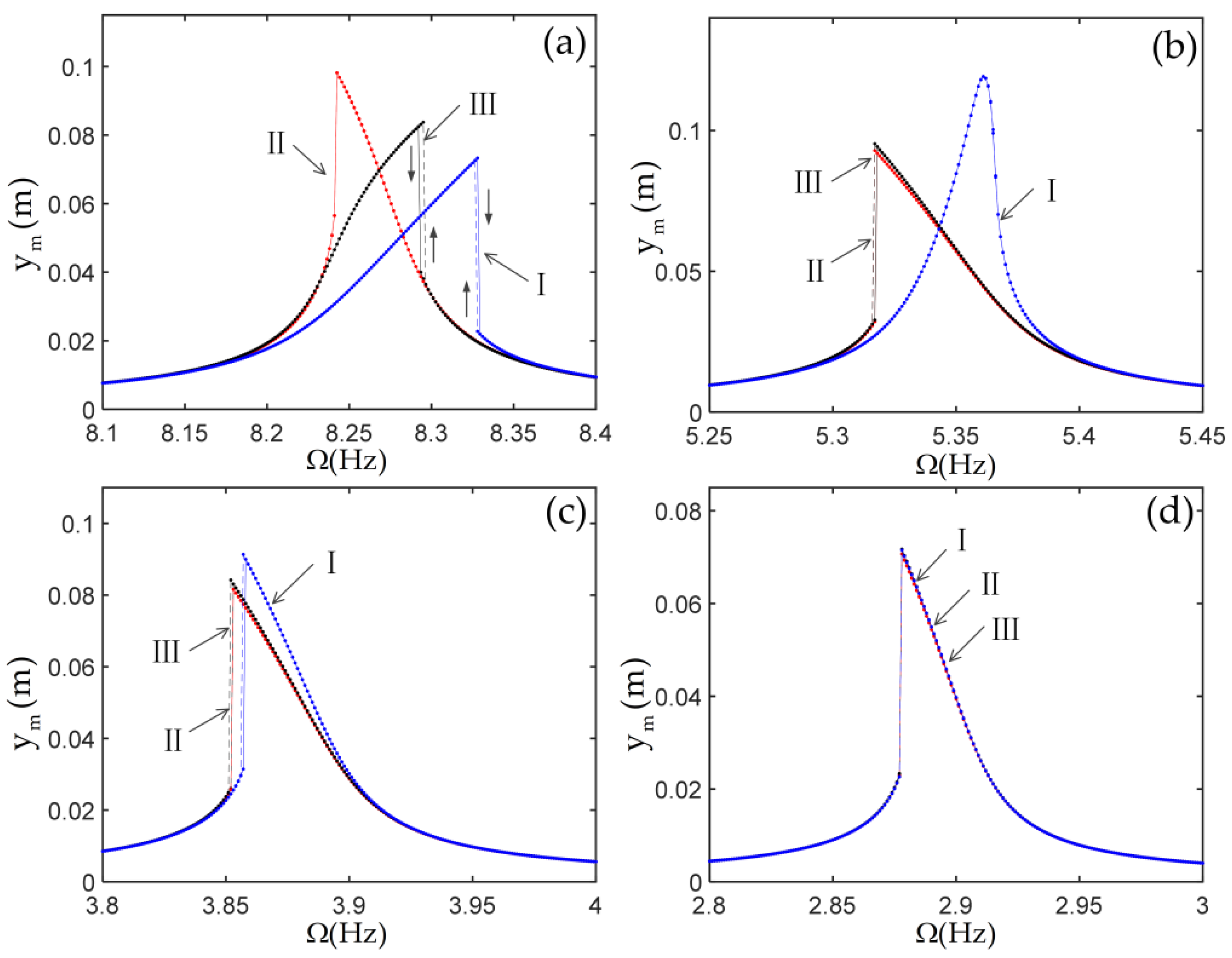
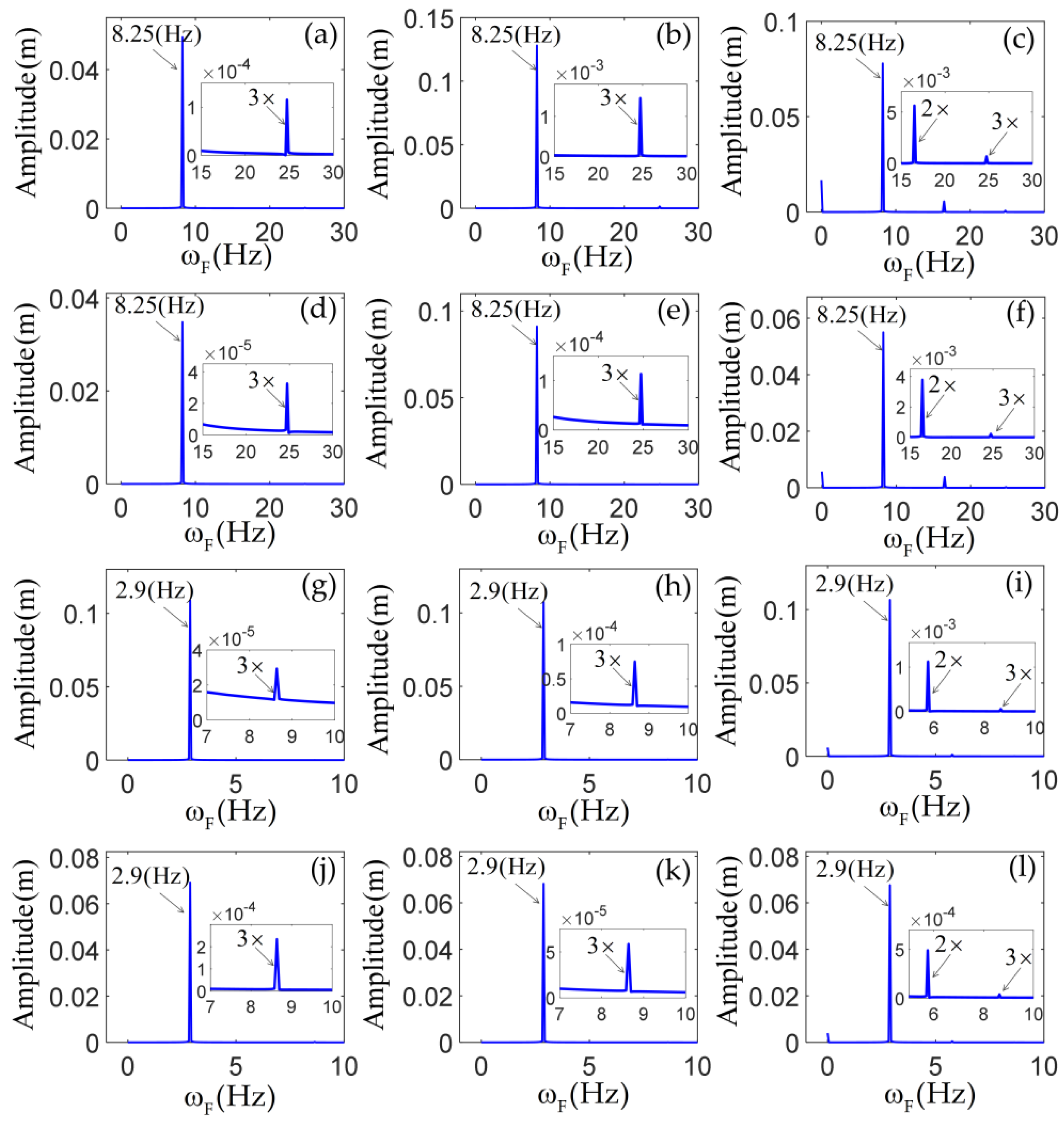
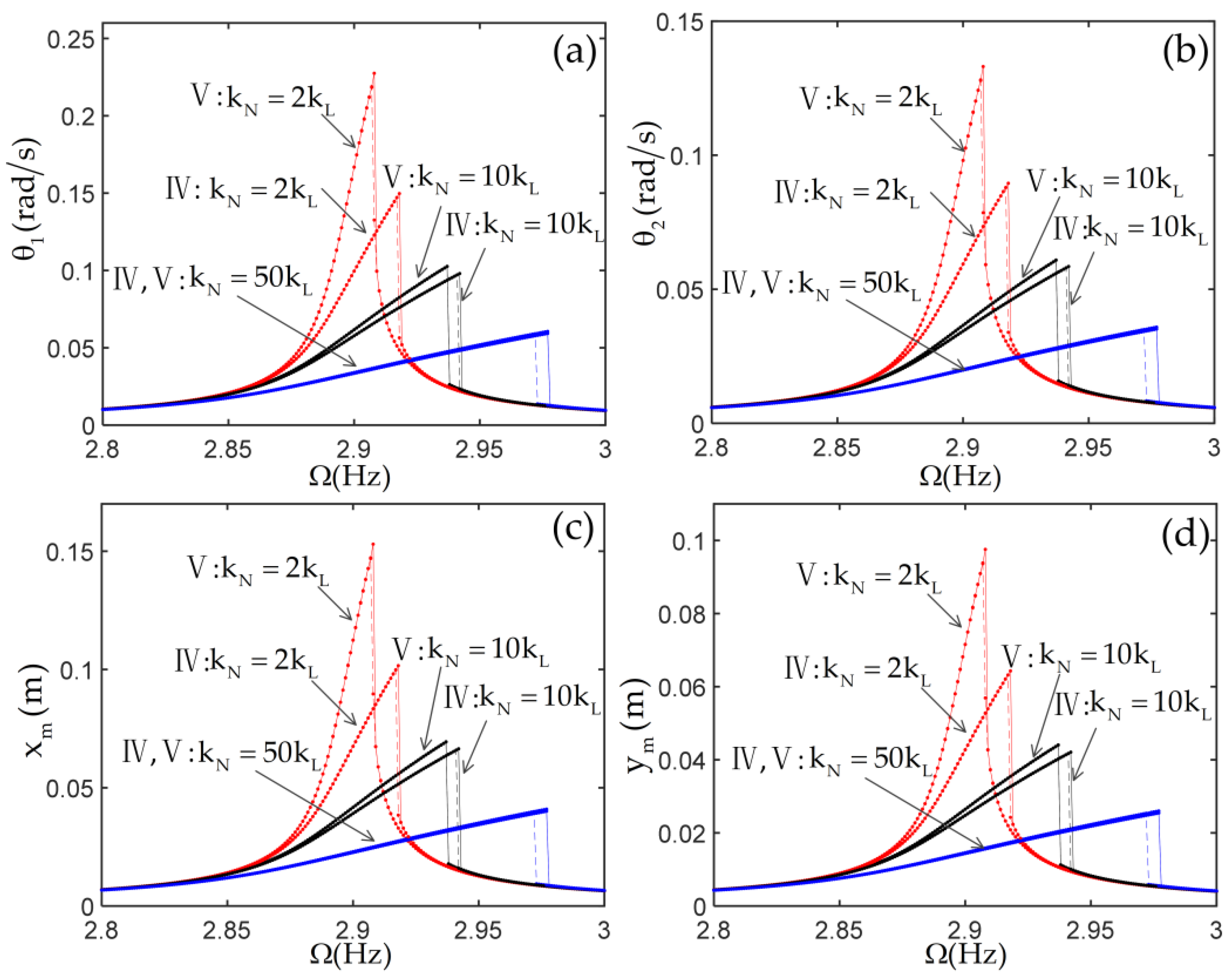
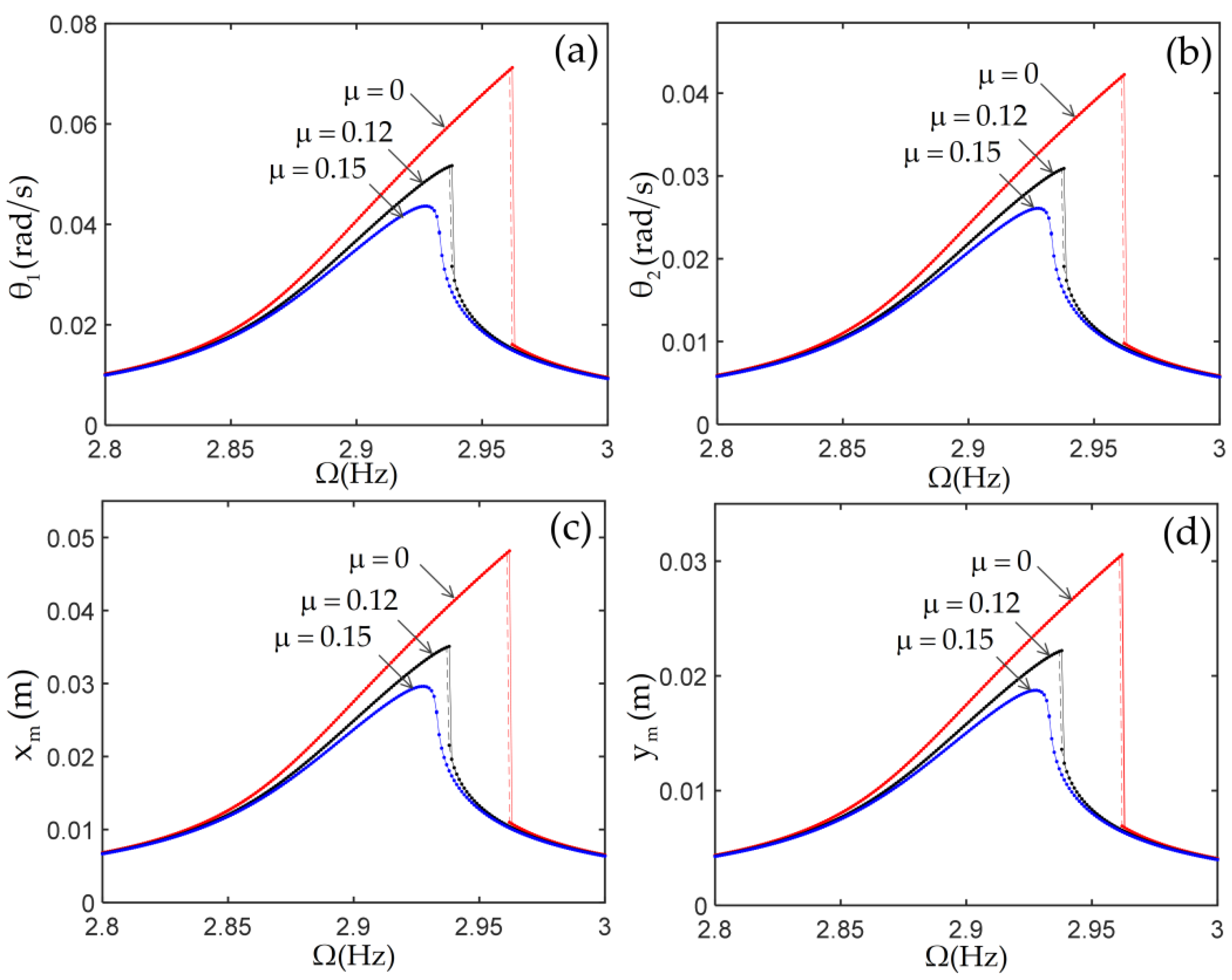
3.2. Nonlinear Responses
4. Conclusions
Author Contributions
Funding
Institutional Review Board Statement
Informed Consent Statement
Data Availability Statement
Conflicts of Interest
Appendix A
Appendix B
References
- Cao, Y.; Cao, D.; He, G.; Ge, X.; Hao, Y. Vibration analysis and distributed piezoelectric energy harvester design for the L-shaped beam. Eur. J. Mech. A-Solid 2021, 87, 104214. [Google Scholar] [CrossRef]
- Li, H.; Sun, H.; Song, B.; Zhang, D.; Shang, X.; Liu, D. Nonlinear dynamic response of an L-shaped beam-mass piezoelectric energy harvester. J. Sound Vibr. 2021, 499, 116004. [Google Scholar] [CrossRef]
- Sharifi-Moghaddam, S.; Tikani, R.; Ziaei-Rad, S. Energy harvesting from nonlinear vibrations of an L-shaped beam using piezoelectric patches. J. Braz. Soc. Mech. Sci. 2021, 43, 1–15. [Google Scholar] [CrossRef]
- Haddow, A.G.; Barr, A.D.S.; Mook, D.T. Theoretical and experimental study of modal interaction in a two-degree-of-freedom structure. J. Sound Vibr. 1984, 97, 451–473. [Google Scholar] [CrossRef]
- Nayfeh, A.H.; Balachandran, B.; Colbert, M.A.; Nayfeh, M.A. An Experimental Investigation of Complicated Responses of a Two-Degree-of-Freedom Structure. J. Appl. Mech.-Trans. ASME 1989, 56, 960–967. [Google Scholar] [CrossRef]
- Balachandran, B.; Nayfeh, A.H. Nonlinear motions of beam-mass structure. Nonlinear Dyn. 1990, 1, 39–61. [Google Scholar] [CrossRef]
- Balachandran, B.; Nayfeh, A.H. Observations of modal interactions in resonantly forced beam-mass structures. Nonlinear Dyn. 1991, 2, 77–117. [Google Scholar] [CrossRef]
- Warminski, J.; Cartmell, M.P.; Bochenski, M.; Ivanov, I. Analytical and experimental investigations of an autoparametric beam structure. J. Sound Vibr. 2008, 315, 486–508. [Google Scholar] [CrossRef]
- Cao, D.; Zhang, W.; Yao, M. Analytical and experimental studies on nonlinear characteristics of an L-shape beam structure. Acta Mech. Sin. 2010, 26, 967–976. [Google Scholar] [CrossRef]
- Onozato, N.; Nagai, K.; Maruyama, S.; Yamaguchi, T. Chaotic vibrations of a post-buckled L-shaped beam with an axial constraint. Nonlinear Dyn. 2012, 67, 2363–2379. [Google Scholar] [CrossRef]
- Georgiades, F.; Warminski, J.; Cartmell, M.P. Towards linear modal analysis for an L-shaped beam: Equations of motion. Mech. Res. Commun. 2013, 47, 50–60. [Google Scholar] [CrossRef] [Green Version]
- Georgiades, F. Nonlinear equations of motion of L-shaped beam structures. Eur. J. Mech. A-Solids 2017, 65, 91–122. [Google Scholar] [CrossRef]
- Wei, J.; Cao, D.; Yang, Y.; Huang, W. Nonlinear Dynamical Modeling and Vibration Responses of an L-Shaped Beam-Mass Structure. J. Appl. Nonlinear Dyn. 2017, 1, 91–104. [Google Scholar] [CrossRef]
- Yu, T.; Zhang, W.; Yang, X. Global bifurcations and chaotic motions of a flexible multi-beam structure. Int. J. Non-Linear Mech. 2017, 95, 264–271. [Google Scholar] [CrossRef]
- Yu, T.; Zhang, W.; Yang, X. Global dynamics of an autoparametric beam structure. Nonlinear Dyn. 2017, 88, 1329–1343. [Google Scholar] [CrossRef]
- Spong, M.W. Modeling and Control of Elastic Joint Robots. J. Dyn. Syst. Meas. Control-Trans. ASME 1987, 109, 310–319. [Google Scholar] [CrossRef]
- Subudhi, B.; Morris, A.S. Dynamic modelling, simulation and control of a manipulator with flexible links and joints. Robot. Auton. Syst. 2002, 41, 257–270. [Google Scholar] [CrossRef]
- Vakil, M.; Fotouhi, R.; Nikiforuk, P.N.; Heidari, F. A study of the free vibration of flexible-link flexible-joint manipulators. Proc. Inst. Mech. Eng. Part J-J. Eng. Tribol. 2011, 225, 1361–1371. [Google Scholar] [CrossRef]
- Meng, D.; She, Y.; Xu, W.; Lu, W.; Liang, B. Dynamic modeling and vibration characteristics analysis of flexible-link and flexible-joint space manipulator. Multibody Syst. Dyn. 2018, 43, 321–347. [Google Scholar] [CrossRef]
- Yang, T.; Yan, S.; Ma, W.; Han, Z. Joint dynamic analysis of space manipulator with planetary gear train transmission. Robotica 2016, 34, 1042–1058. [Google Scholar] [CrossRef]
- Yang, T.; Yan, S.; Han, Z. Nonlinear model of space manipulator joint considering time-variant stiffness and backlash. J. Sound Vibr. 2015, 341, 246–259. [Google Scholar] [CrossRef]
- Wei, J.; Cao, D.; Lun, L.; Huang, W. Global mode method for dynamic modeling of a flexible-link flexible-joint manipulator with tip mass. Appl. Math. Model. 2017, 48, 787–805. [Google Scholar] [CrossRef]
- Moon, F.C.; Li, G.X. Experimental study of chaotic vibrations in a pin-jointed space truss structure. AIAA J. 1990, 28, 915–921. [Google Scholar] [CrossRef]
- Folkman, S.L.; Rowsell, E.A.; Ferney, G.D. Influence of pinned joints on damping and dynamic behavior of a truss. J. Guid. Control Dyn. 1995, 18, 1398–1403. [Google Scholar] [CrossRef]
- Bowden, M.; Dugundji, J. Joint damping and nonlinearity in dynamics of space structures. AIAA J. 1990, 28, 740–749. [Google Scholar] [CrossRef]
- Zhang, J.; Guo, H.; Liu, R.; Wu, J.; Kou, Z.; Deng, Z. Damping formulations for jointed deployable space structures. Nonlinear Dyn. 2015, 81, 1969–1980. [Google Scholar] [CrossRef]
- Guo, H.; Zhang, J.; Liu, R.; Deng, Z. Effects of Joint on Dynamics of Space Deployable Structure. Chin. J. Mech. Eng. 2013, 26, 861–872. [Google Scholar] [CrossRef]
- Wei, J.; Cao, D.; Huang, H.; Wang, L.; Huang, W. Dynamics of a multi-beam structure connected with nonlinear joints: Modelling and simulation. Arch. Appl. Mech. 2018, 88, 1059–1074. [Google Scholar] [CrossRef]
- Wei, J.; Cao, D.; Huang, H. Nonlinear vibration phenomenon of maneuvering spacecraft with flexible jointed appendages. Nonlinear Dyn. 2018, 94, 2813–2877. [Google Scholar] [CrossRef]
- Esmailzadeh, A.E.; Jalili, A.N. Parametric response of cantilever Timoshenko beams with tip mass under harmonic support motion. Int. J. Non-Linear Mech. 1998, 33, 765–781. [Google Scholar] [CrossRef]
- Yabuno, H.; Ide, Y.; Aoshima, N. Nonlinear Analysis of a Parametrically Excited Cantilever Beam. (Effect of the Tip Mass on Stationary Response). JSME Int. J. Ser. C-Mech. Syst. Mach. Elem. Manuf. 1998, 41, 555–562. [Google Scholar] [CrossRef] [Green Version]
- Eftekhari, M.; Mahzoon, M.; Ziaei-Rad, S. Effect of added tip mass on the nonlinear flapwise and chordwise vibration of cantilever composite beam under base excitation. Int. J. Struct. Stab. Dyn. 2012, 12, 285–310. [Google Scholar] [CrossRef]
- Cheng, G.; Mei, C.; Lee, R. Large Amplitude Vibration of a Cantilever Beam with Tip Mass Under Random Base Excitation. Adv. Struct. Eng. 2001, 4, 203–210. [Google Scholar] [CrossRef]
- Meesala, V.C.; Hajj, M.R. Parameter sensitivity of cantilever beam with tip mass to parametric excitation. Nonlinear Dyn. 2019, 95, 3375–3384. [Google Scholar] [CrossRef]


| Parameter | Value |
|---|---|
| 7800 | |
| 200 | |
| (m) | 0.02 |
| (m) | 0.005 |
| (m) | 0.3 |
| 0.01 | |
| 138.5 |
Publisher’s Note: MDPI stays neutral with regard to jurisdictional claims in published maps and institutional affiliations. |
© 2021 by the authors. Licensee MDPI, Basel, Switzerland. This article is an open access article distributed under the terms and conditions of the Creative Commons Attribution (CC BY) license (https://creativecommons.org/licenses/by/4.0/).
Share and Cite
Wei, J.; Yu, T.; Jin, D.; Liu, M.; Cao, D.; Wang, J. Nonlinear Dynamic Modeling and Analysis of an L-Shaped Multi-Beam Jointed Structure with Tip Mass. Materials 2021, 14, 7279. https://doi.org/10.3390/ma14237279
Wei J, Yu T, Jin D, Liu M, Cao D, Wang J. Nonlinear Dynamic Modeling and Analysis of an L-Shaped Multi-Beam Jointed Structure with Tip Mass. Materials. 2021; 14(23):7279. https://doi.org/10.3390/ma14237279
Chicago/Turabian StyleWei, Jin, Tao Yu, Dongping Jin, Mei Liu, Dengqing Cao, and Jinjie Wang. 2021. "Nonlinear Dynamic Modeling and Analysis of an L-Shaped Multi-Beam Jointed Structure with Tip Mass" Materials 14, no. 23: 7279. https://doi.org/10.3390/ma14237279
APA StyleWei, J., Yu, T., Jin, D., Liu, M., Cao, D., & Wang, J. (2021). Nonlinear Dynamic Modeling and Analysis of an L-Shaped Multi-Beam Jointed Structure with Tip Mass. Materials, 14(23), 7279. https://doi.org/10.3390/ma14237279