
Electrospinning Processing Techniques for the Manufacturing of Composite Dielectric Elastomer Fibers


Abstract
:1. Introduction
2. Materials and Methods
3. Modeling of Electrospinning Process
4. Results and Discussion
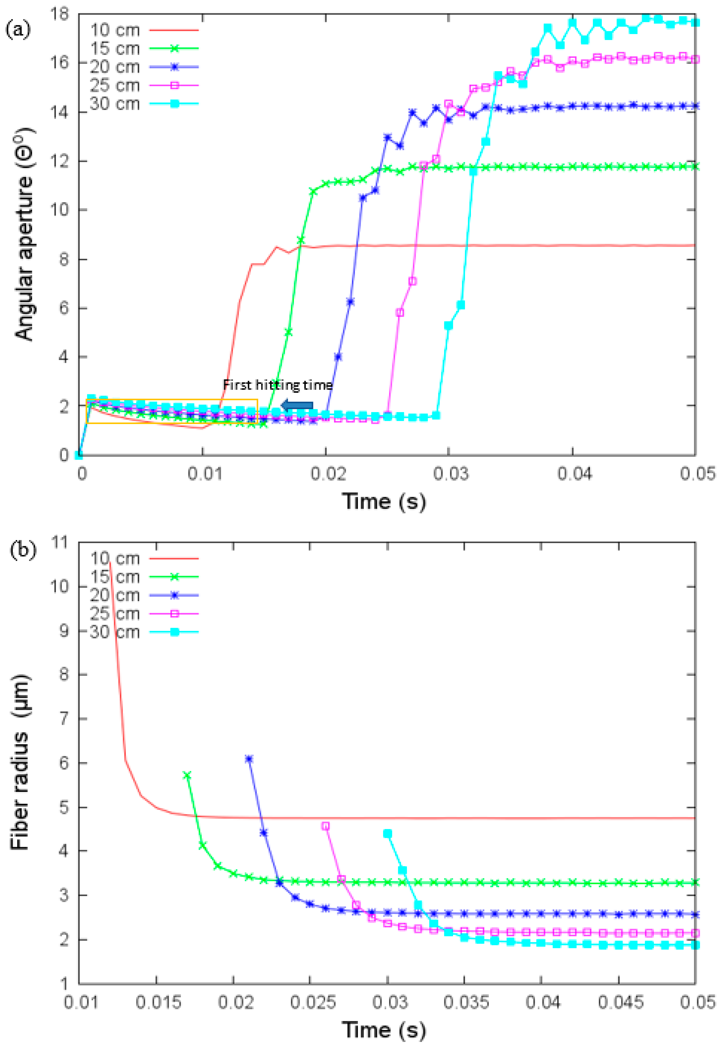
4.1. Effect of Collector Distance
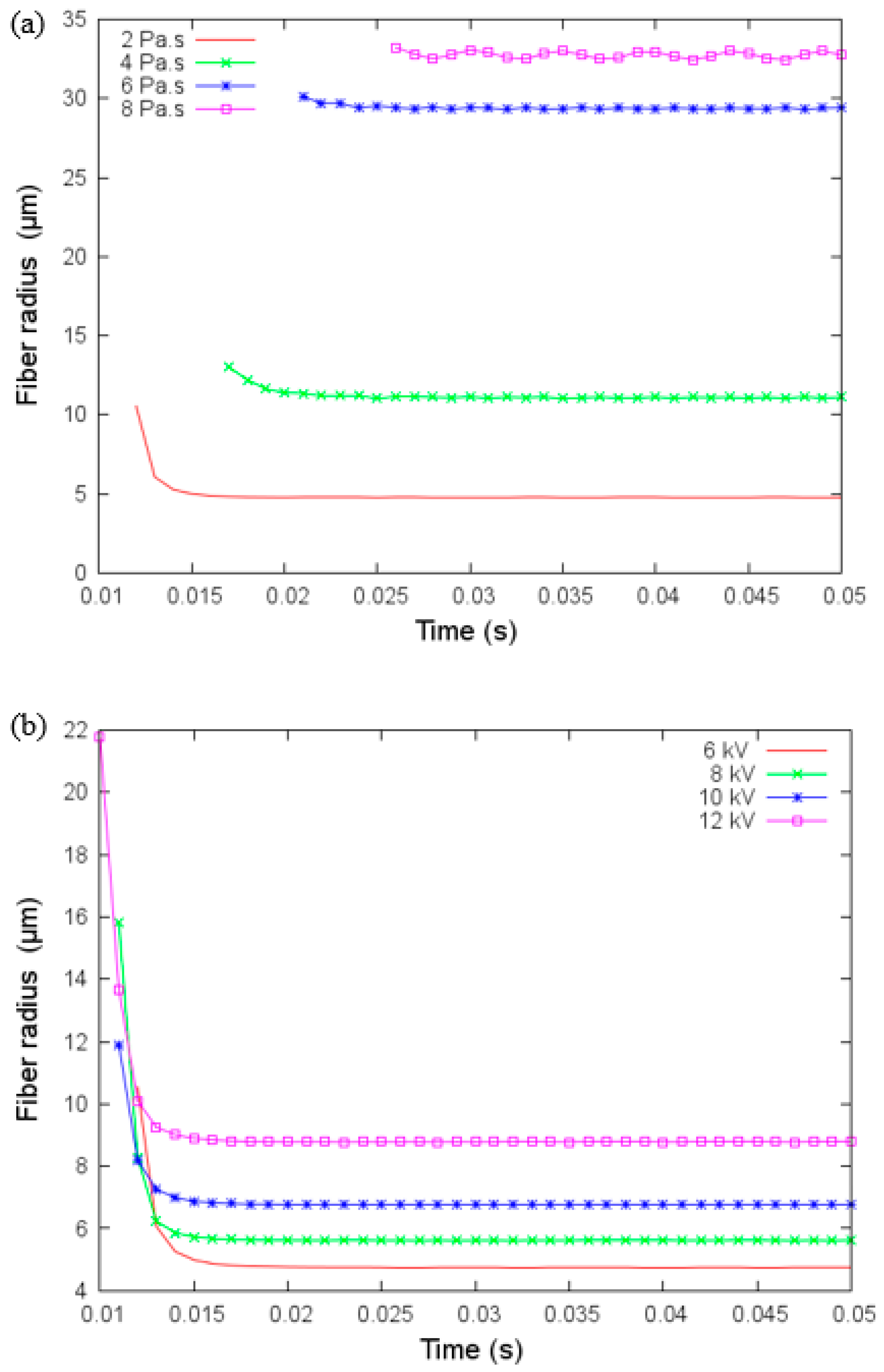
4.2. Effect of Viscosity and Applied Voltage
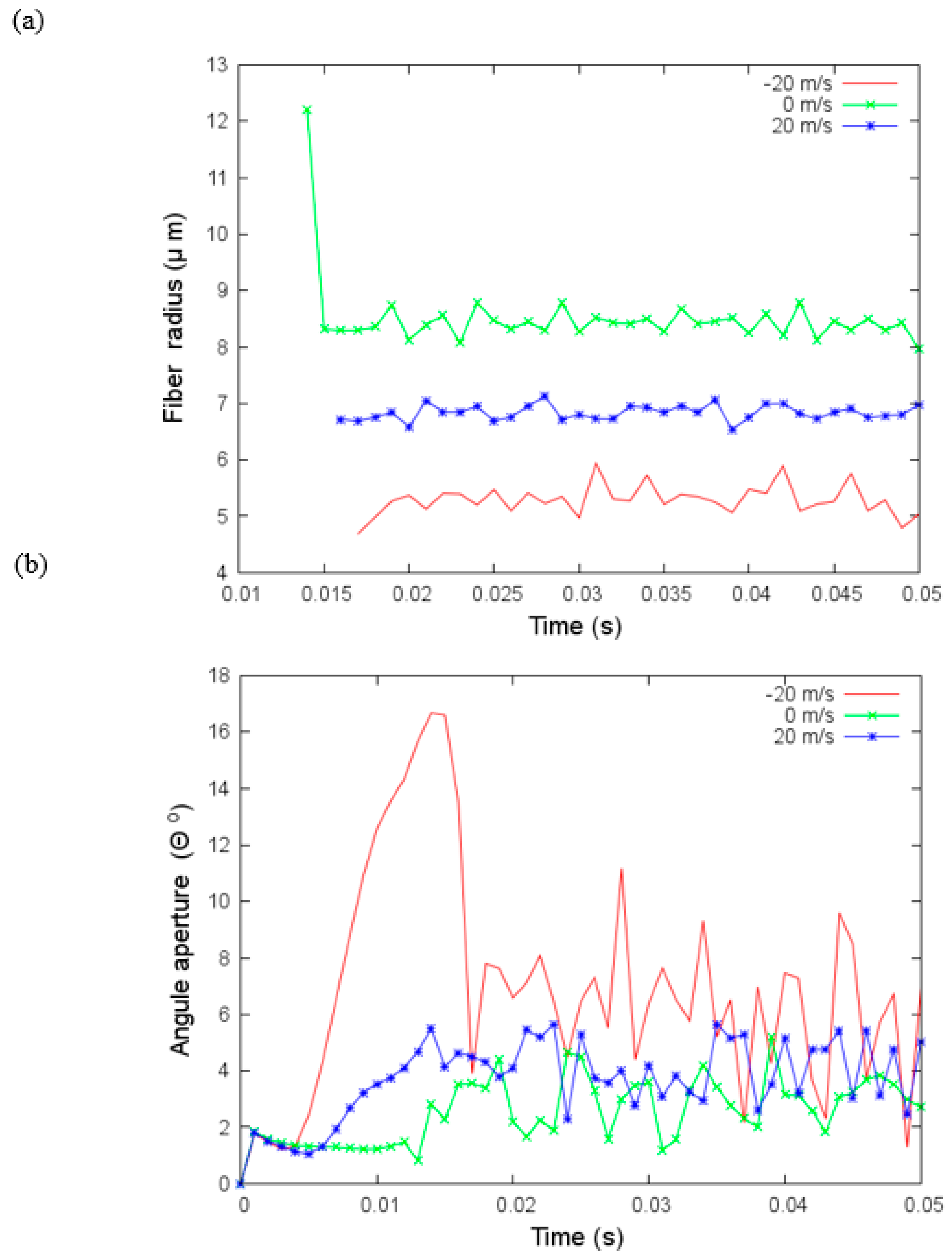
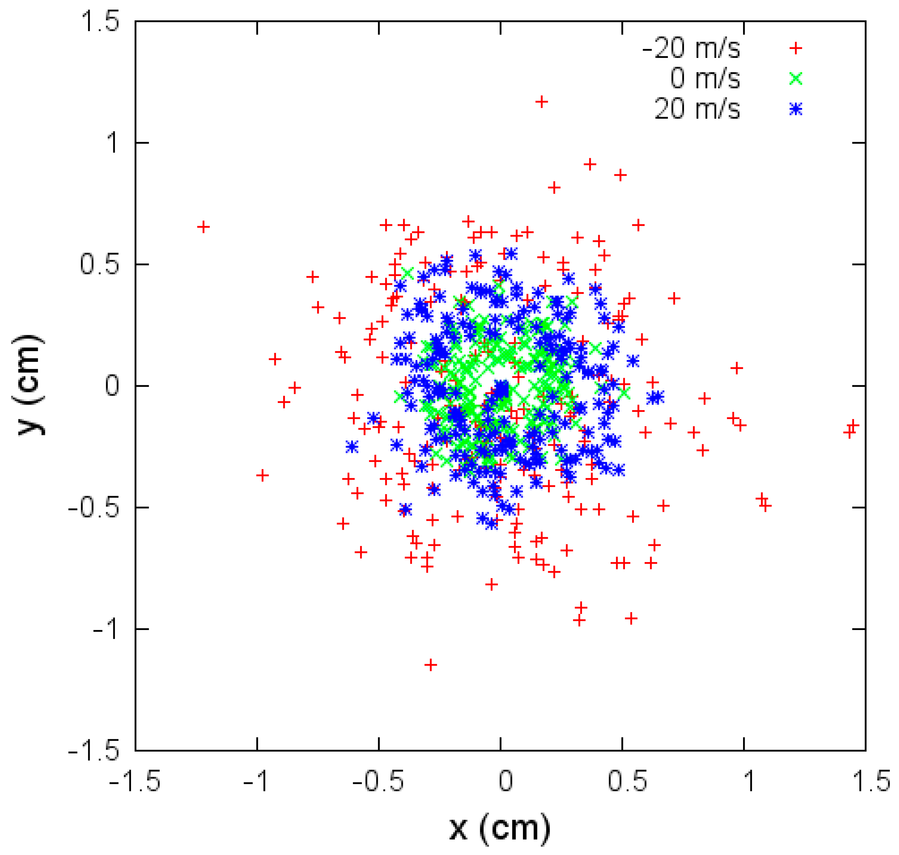
4.3. Effect of Air Drag on Polymer Jet
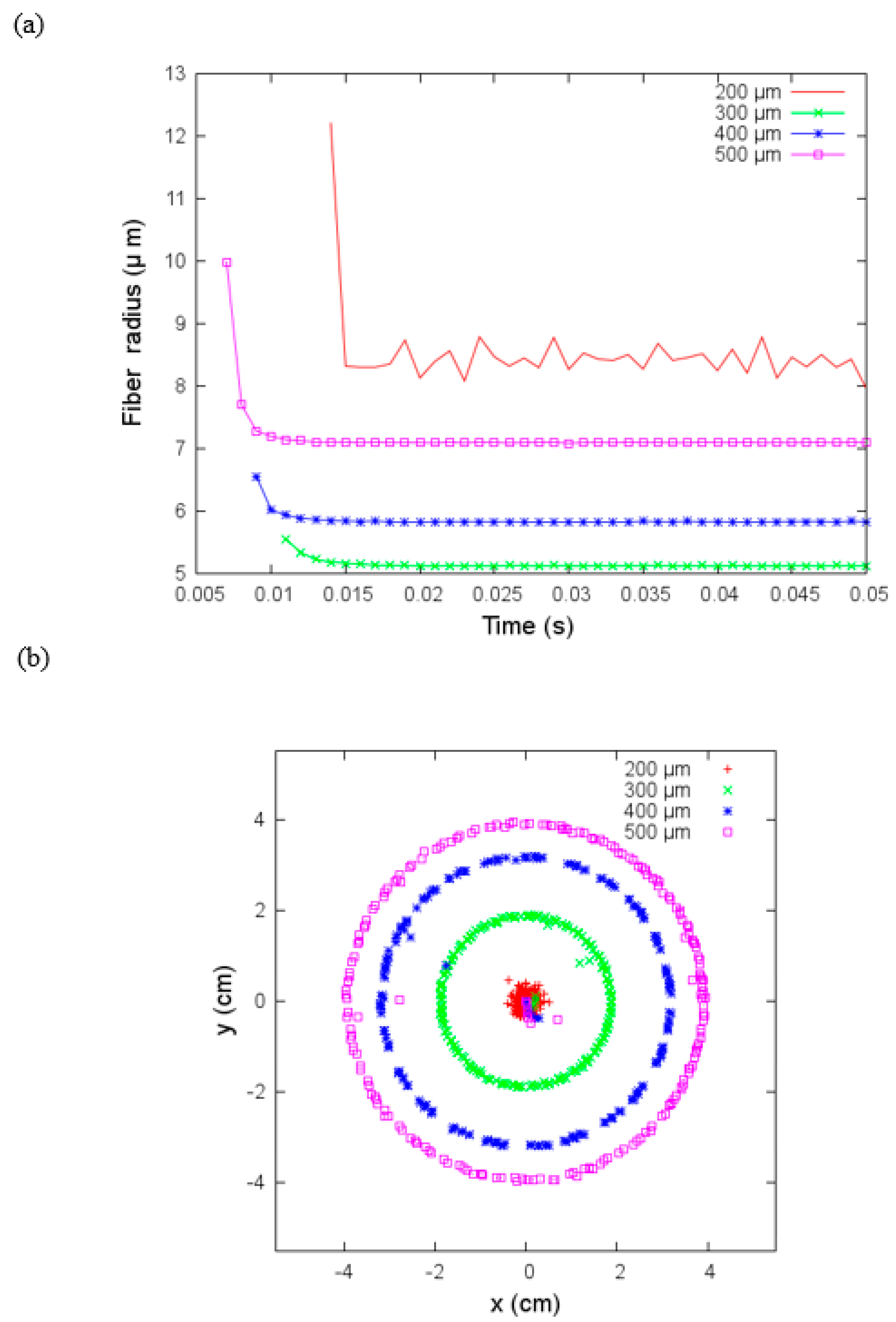
4.4. Effect of Nozzle Radius
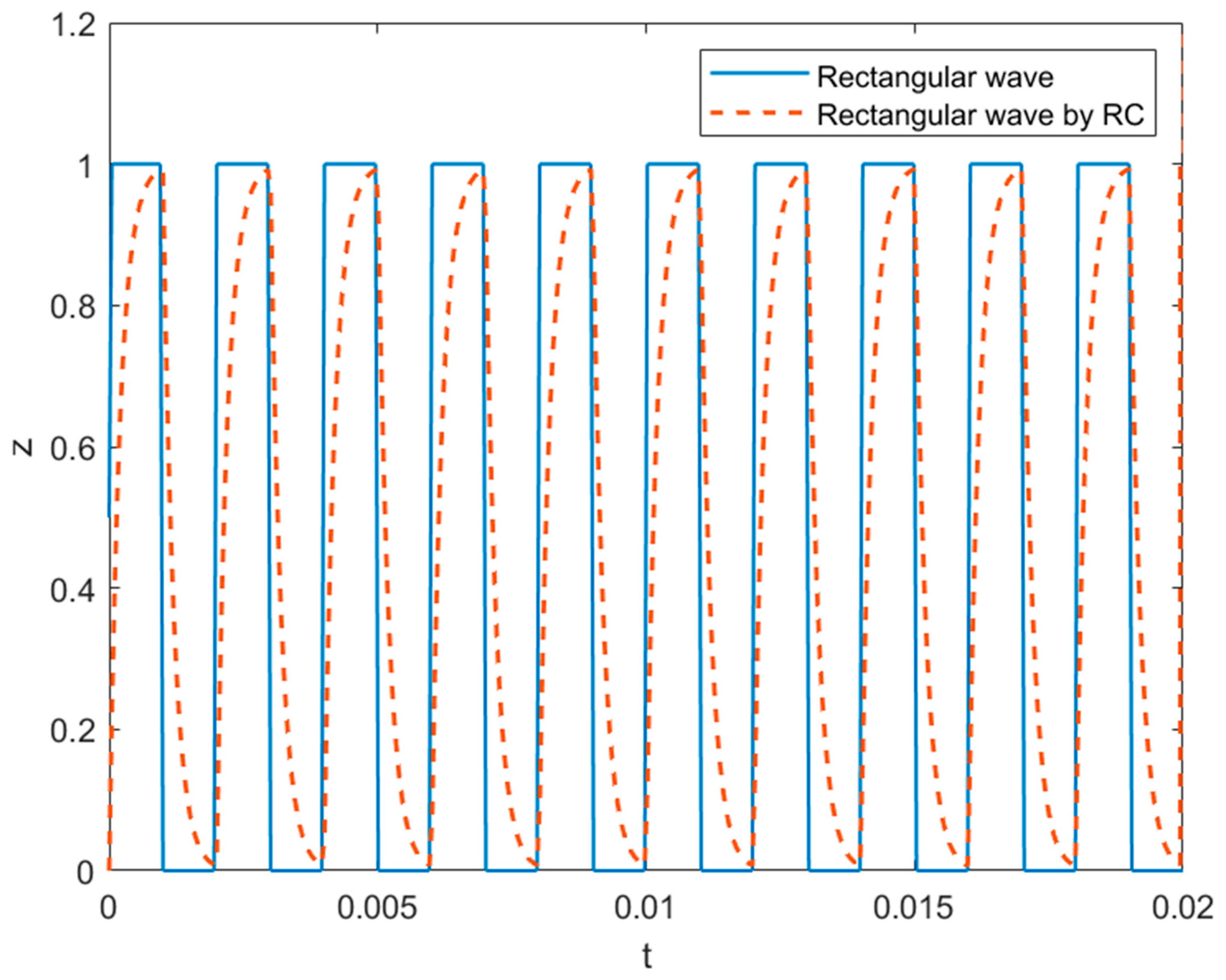
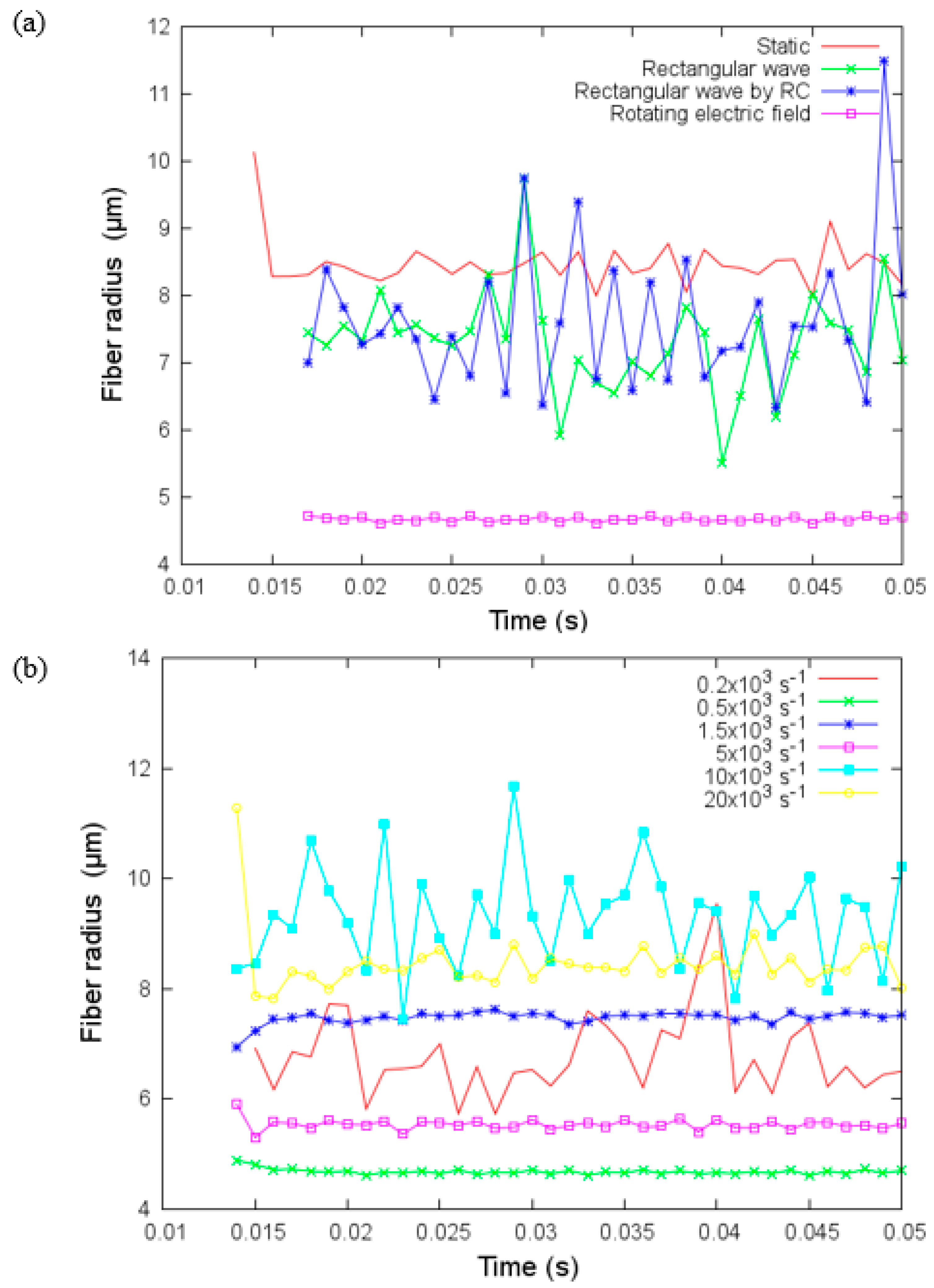
4.5. Effect of AC Electrospinning
4.6. Correlation to Experimental Observations
5. Conclusions
Author Contributions
Funding
Institutional Review Board Statement
Informed Consent Statement
Data Availability Statement
Conflicts of Interest
References
- Arora, S.; Ghosh, T.; Muth, J. Dielectric elastomer based prototype fiber actuators. Sens. Actuators A Phys. 2007, 136, 321–328. [Google Scholar] [CrossRef]
- Bar-Cohen. Electrochemistry Encyclopedia. Clevel. Ohio. 2002. Available online: http://electrochem.cwru.edu/encycl/ (accessed on 1 September 2021).
- Qiu, Y.; Zhang, E.; Plamthottam, R.; Pei, Q. Dielectric elastomer artificial muscle: Materials innovations and device explorations. Acc. Chem. Res. 2019, 52, 316–325. [Google Scholar] [CrossRef] [PubMed]
- Pan, S.; Dai, Q.; Safaei, B.; Qin, Z.; Chu, F. Damping characteristics of carbon nanotube reinforced epoxy nanocomposite beams. Thin-Walled Struct. 2021, 166, 108127. [Google Scholar] [CrossRef]
- Zu, X.; Wu, H.; Lv, H.; Zheng, Y.; Li, H. An amplitude-and temperature-dependent vibration model of fiber-reinforced composite thin plates in a thermal environment. Materials 2020, 13, 1590. [Google Scholar] [CrossRef] [PubMed] [Green Version]
- Wang, X.-X.; Yu, G.-F.; Zhang, J.; Yu, M.; Ramakrishna, S.; Long, Y.-Z. Conductive polymer ultrafine fibers via electrospinning: Preparation, physical properties and applications. Prog. Mater. Sci. 2021, 115, 100704. [Google Scholar] [CrossRef]
- Robinson, A.J.; Pérez-Nava, A.; Ali, S.C.; González-Campos, J.B.; Holloway, J.L.; Cosgriff-Hernandez, E.M. Comparative analysis of fiber alignment methods in electrospinning. Matter 2021, 4, 821–844. [Google Scholar] [CrossRef]
- Grasl, C.; Stoiber, M.; Röhrich, M.; Moscato, F.; Bergmeister, H.; Schima, H. Electrospinning of small diameter vascular grafts with preferential fiber directions and comparison of their mechanical behavior with native rat aortas. Mater. Sci. Eng. C 2021, 124, 112085. [Google Scholar] [CrossRef] [PubMed]
- Ge, L.; Yin, J.; Yan, D.; Hong, W.; Jiao, T. Construction of nanocrystalline cellulose-based composite fiber films with excellent porosity performances via an electrospinning strategy. ACS Omega 2021, 6, 4958–4967. [Google Scholar] [CrossRef] [PubMed]
- Uslu, E.; Gavgali, M.; Erdal, M.O.; Yazman, Ş.; Gemi, L. Determination of mechanical properties of polymer matrix composites reinforced with electrospinning N66, PAN, PVA and PVC nanofibers: A comparative study. Mater. Today Commun. 2021, 26, 101939. [Google Scholar] [CrossRef]
- Guo, H.; Chen, Y.; Li, Y.; Zhou, W.; Xu, W.; Pang, L.; Fan, X.; Jiang, S. Electrospun fibrous materials and their applications for electromagnetic interference shielding: A review. Compos. Part A Appl. Sci. Manuf. 2021, 143, 106309. [Google Scholar] [CrossRef]
- Ji, R.; Zhang, Q.; Zhou, F.; Xu, F.; Wang, X.; Huang, C.; Zhu, Y.; Zhang, H.; Sun, L.; Xia, Y. Electrospinning fabricated novel poly (ethylene glycol)/graphene oxide composite phase-change nano-fibers with good shape stability for thermal regulation. J. Energy Storage 2021, 40, 102687. [Google Scholar] [CrossRef]
- Grant, J.J.; Pillai, S.C.; Perova, T.S.; Hehir, S.; Hinder, S.J.; McAfee, M.; Breen, A. Electrospun Fibres of Chitosan/PVP for the Effective Chemotherapeutic Drug Delivery of 5-Fluorouracil. Chemosensors 2021, 9, 70. [Google Scholar] [CrossRef]
- Nobeshima, T.; Ishii, Y.; Sakai, H.; Uemura, S.; Yoshida, M. Actuation behavior of polylactic acid fiber films prepared by electrospinning. J. Nanosci. Nanotechnol. 2016, 16, 3343–3348. [Google Scholar] [CrossRef] [PubMed]
- Tian, M.; Yao, Y.; Liu, S.; Yang, D.; Zhang, L.; Nishi, T.; Ning, N. Separated-structured all-organic dielectric elastomer with large actuation strain under ultra-low voltage and high mechanical strength. J. Mater. Chem. A 2015, 3, 1483–1491. [Google Scholar] [CrossRef]
- Jiang, L.; Zhou, Y.; Wang, Y.; Jiang, Z.; Zhou, F.; Chen, S.; Ma, J. Fabrication of dielectric elastomer composites by locking a pre-stretched fibrous TPU network in EVA. Materials 2018, 11, 1687. [Google Scholar] [CrossRef] [PubMed] [Green Version]
- Bhattarai, N.; Edmondson, D.; Veiseh, O.; Matsen, F.A.; Zhang, M. Electrospun chitosan-based nanofibers and their cellular compatibility. Biomaterials 2005, 26, 6176–6184. [Google Scholar] [CrossRef] [PubMed]
- Li, D.; Wang, Y.; Xia, Y. Electrospinning nanofibers as uniaxially aligned arrays and layer-by-layer stacked films. Adv. Mater. 2004, 16, 361–366. [Google Scholar] [CrossRef]
- Kulkarni, A.; Bambole, V.; Mahanwar, P. Electrospinning of polymers, their modeling and applications. Polym.-Plast. Technol. Eng. 2010, 49, 427–441. [Google Scholar] [CrossRef]
- Rafiei, S.; Maghsoodloo, S.; Noroozi, B.; Mottaghitalab, V.; Haghi, A. Mathematical modeling in electrospinning process of nanofibers: A detailed review. Cellul. Chem. Technol. 2013, 47, 323–338. [Google Scholar]
- Carroll, C.P.; Joo, Y.L. Electrospinning of viscoelastic Boger fluids: Modeling and experiments. Phys. Fluids 2006, 18, 053102. [Google Scholar] [CrossRef]
- Yousefzadeh, M. Modeling and simulation of the electrospinning process. In Electrospun Nanofibers; Elsevier: Amsterdam, The Netherlands, 2017; pp. 277–301. [Google Scholar]
- Kowalewski, T.A.; Barral, S.; Kowalczyk, T. Modeling electrospinning of nanofibers. In Proceedings of the IUTAM symposium on Modelling Nanomaterials and Nanosystems, Aalborg, Denmark, 19–22 May 2008; pp. 279–292. [Google Scholar]
- Karra, S. Modeling Electrospinning Process and a Numerical Scheme Using Lattice Boltzmann Method to Simulate Viscoelastic fluid flows. Ph.D. Thesis, Texas A & M University, College Station, TX, USA, 2010. [Google Scholar]
- Karatay, O.; Dogan, M. Modelling of electrospinning process at various electric fields. Micro Nano Lett. 2011, 6, 858–862. [Google Scholar] [CrossRef]
- Khatti, T.; Naderi-Manesh, H.; Kalantar, S.M. Application of ANN and RSM techniques for modeling electrospinning process of polycaprolactone. Neural Comput. Appl. 2019, 31, 239–248. [Google Scholar] [CrossRef]
- Lauricella, M.; Pisignano, D.; Succi, S. Three-Dimensional Model for Electrospinning Processes in Controlled Gas Counterflow. J. Phys. Chem. A 2016, 120, 4884–4892. [Google Scholar] [CrossRef] [PubMed] [Green Version]
- Wu, X.-F.; Salkovskiy, Y.; Dzenis, Y.A. Modeling of solvent evaporation from polymer jets in electrospinning. Appl. Phys. Lett. 2011, 98, 223108. [Google Scholar] [CrossRef] [Green Version]
- Liu, L.-G.; He, J.-H. Solvent evaporation in a binary solvent system for controllable fabrication of porous fibers by electrospinning. Therm. Sci. 2017, 21, 1821–1825. [Google Scholar] [CrossRef] [Green Version]
- Lauricella, M.; Pontrelli, G.; Coluzza, I.; Pisignano, D.; Succi, S. JETSPIN: A specific-purpose open-source software for simulations of nanofiber electrospinning. Comput. Phys. Commun. 2015, 197, 227–238. [Google Scholar] [CrossRef]
- Montinaro, M.; Fasano, V.; Moffa, M.; Camposeo, A.; Persano, L.; Lauricella, M.; Succi, S.; Pisignano, D. Sub-ms dynamics of the instability onset of electrospinning. Soft Matter 2015, 11, 3424–3431. [Google Scholar] [CrossRef] [PubMed] [Green Version]
- Lauricella, M.; Cipolletta, F.; Pontrelli, G.; Pisignano, D.; Succi, S. Effects of orthogonal rotating electric fields on electrospinning process. Phys. Fluids 2017, 29, 082003. [Google Scholar] [CrossRef] [Green Version]


| Shear Rate (mm/s) | SBS Viscosity (cps) | A85 + 30% MWCNT Viscosity (cps) |
|---|---|---|
| 0.196 | 14080 | 4330 |
| 0.392 | 14080 | 5320 |
| 0.982 | 13620 | 5990 |
| 1.96 | 10740 | 7300 |
| 3.92 | 9960 | 9560 |
| 7.85 | 8960 | 16220 |
| 19.6 | 8680 | 16890 |
| Concentration of Solid in Solvent | Distance between Needle and Collector (cm) | Pump Flow Rate (mL/h) | Spinning Voltage (kV) | Diameter Range (µm) |
|---|---|---|---|---|
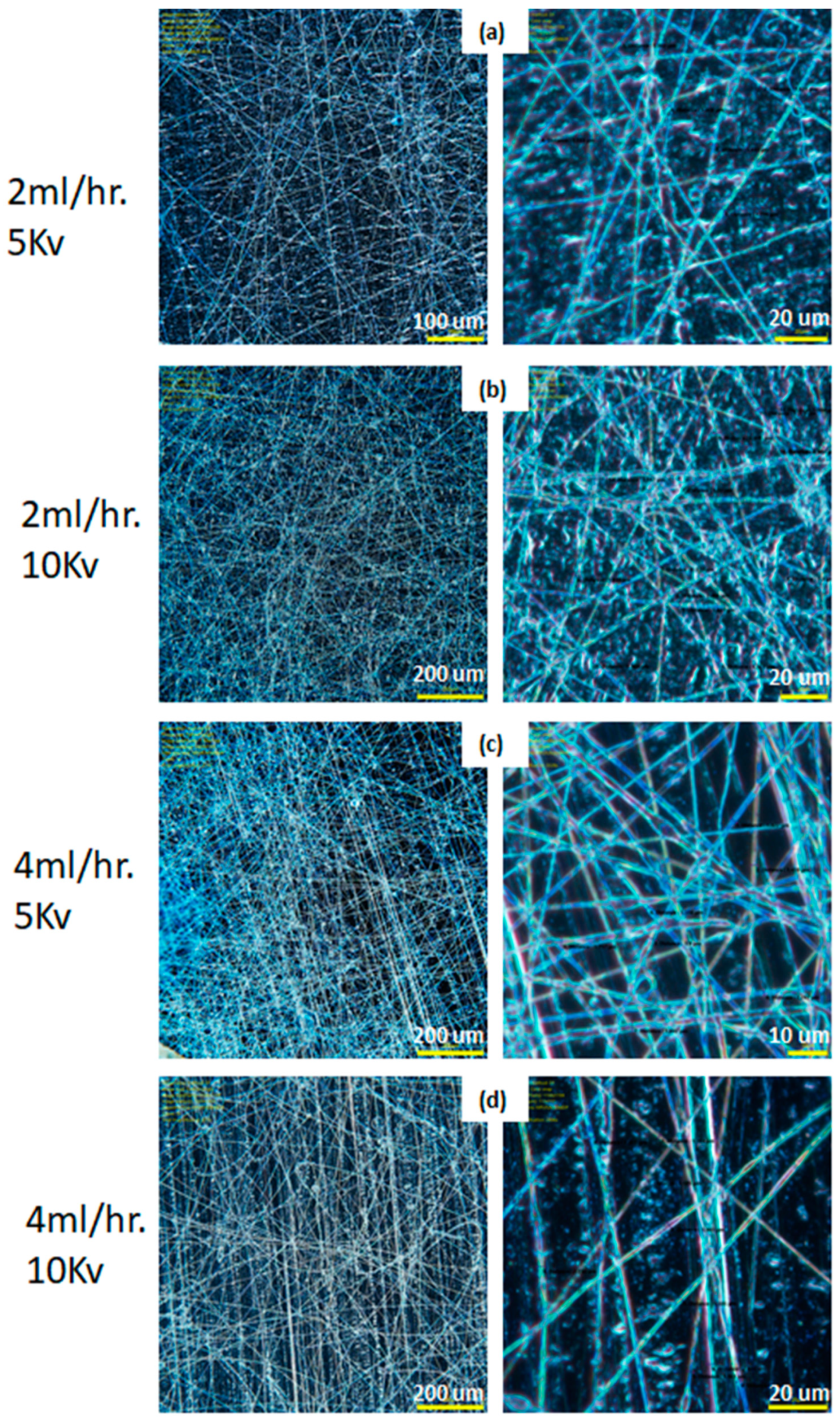
| 30 wt.% | 2.5 | 2 | 5 | 1.5–2.6 |
| 30 wt.% | 2.5 | 2 | 10 | 1.3–2.9 |
| 30 wt.% | 2.5 | 4 | 5 | 1.5–2.8 |
| 30 wt.% | 2.5 | 8 | 10 | 1.3–2.9 |
| Young’s modulus (G) | 1.32 MPa | 6 kV | |
| Distance at the collector (h) | 10 cm | 2.0 Pa·s | |
| 1030 kg/m3 | 40 microns | ||
| 200 microns | 104 s−1 | ||
| 1.21 kg/m3 | 10−3 | ||
| 0.151 cm2/s | 21.1 mN/m |
Publisher’s Note: MDPI stays neutral with regard to jurisdictional claims in published maps and institutional affiliations. |
© 2021 by the authors. Licensee MDPI, Basel, Switzerland. This article is an open access article distributed under the terms and conditions of the Creative Commons Attribution (CC BY) license (https://creativecommons.org/licenses/by/4.0/).
Share and Cite
Ramirez, M.; Vaught, L.; Law, C.; Meyer, J.L.; Elhajjar, R. Electrospinning Processing Techniques for the Manufacturing of Composite Dielectric Elastomer Fibers. Materials 2021, 14, 6288. https://doi.org/10.3390/ma14216288
Ramirez M, Vaught L, Law C, Meyer JL, Elhajjar R. Electrospinning Processing Techniques for the Manufacturing of Composite Dielectric Elastomer Fibers. Materials. 2021; 14(21):6288. https://doi.org/10.3390/ma14216288
Chicago/Turabian StyleRamirez, Mirella, Louis Vaught, Chiu Law, Jacob L. Meyer, and Rani Elhajjar. 2021. "Electrospinning Processing Techniques for the Manufacturing of Composite Dielectric Elastomer Fibers" Materials 14, no. 21: 6288. https://doi.org/10.3390/ma14216288
APA StyleRamirez, M., Vaught, L., Law, C., Meyer, J. L., & Elhajjar, R. (2021). Electrospinning Processing Techniques for the Manufacturing of Composite Dielectric Elastomer Fibers. Materials, 14(21), 6288. https://doi.org/10.3390/ma14216288