
General Consistency of Strong Discontinuity Kinematics in Embedded Finite Element Method (E-FEM) Formulations


Abstract
:
1. Introduction
2. Analysis of Basic Internal Strong Discontinuity Kinematics
2.1. Kinematic Consistency of Boundary Condition Imposition
2.2. Kinematics at Terminal Separation Conditions and Meaning of
3. In-Depth Analysis of Variational Foundations
3.1. A Word on the Discretisation Strategy
3.1.1. Displacement Field Discretisation
3.1.2. Strain Field Discretisation
3.1.3. Stress Field Discretisation
3.1.4. Calculated Stress Field Discretisation
3.2. Application of the Discretisation Strategy
3.2.1. Basic Orthogonality Analysis: The Role of
3.2.2. The Bridge between Real and Constitutive Stress Fields
3.2.3. The Bridge between Real and Constitutive Traction Vectors
3.2.4. EAS and Static Considerations—The Patch Test Condition
3.2.5. Final Traction Calculation
3.2.6. Internal–External Force Balance
4. Current Formulation Approaches and Associated Pathologies
4.1. Single Mode Formulations
4.2. Full Crack Translation Formulations: The Role of
4.3. General Crack Kinematics Formulations
5. Formulation Approach Proposal for Three Dimensional Problems
5.1. A Consistent Enrichment for
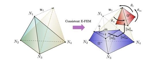
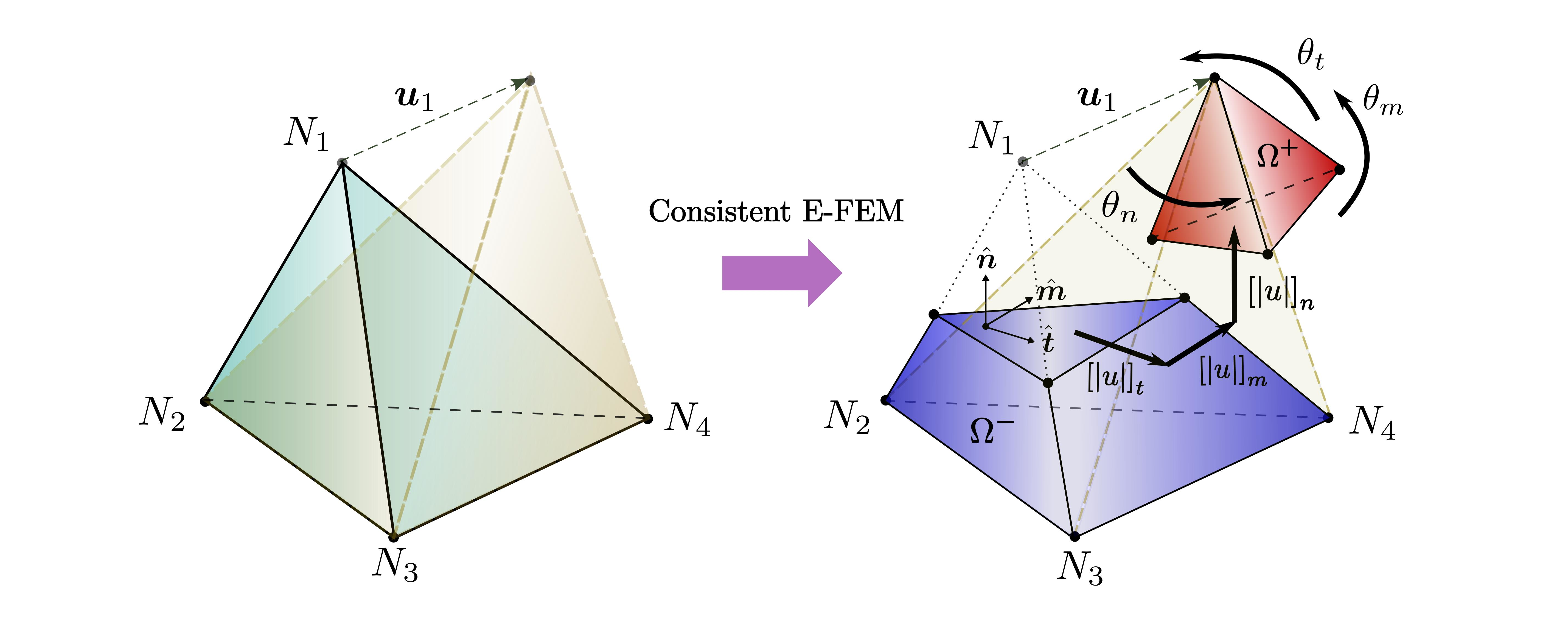
5.2. Fracture Kinematics Enrichment in 3D Coexisting with
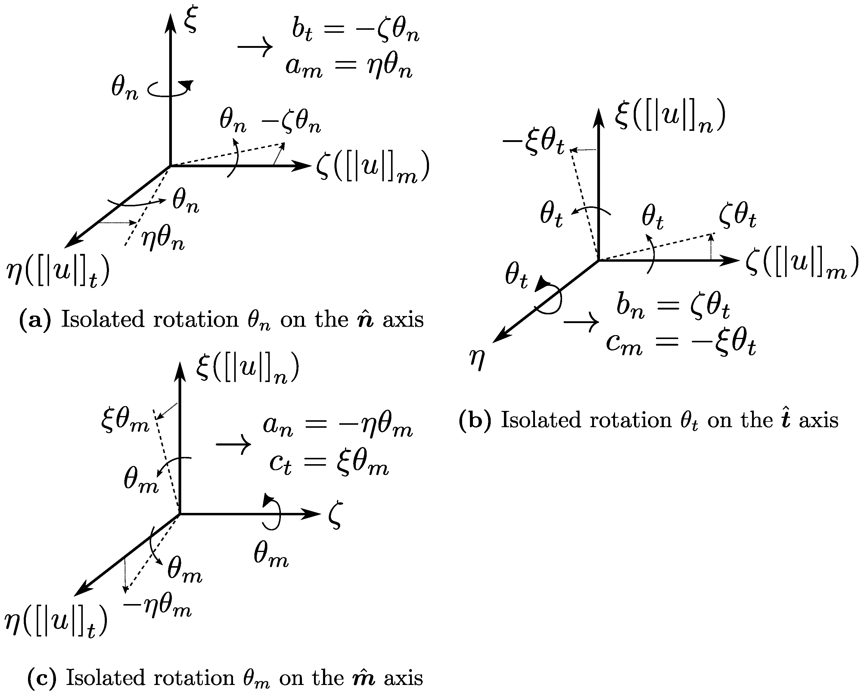
- As mentioned already in Section 2.1, it is not required to have the same structure associated for all fracture displacement components . Indeed, three different functions may coexist in the model:While this might apparently triple the amount of free parameters, some of the model symmetries that are allowed for redundancy simplifications will no longer emerge. As an example, the basic deformation gradient operator on (the first three columns of ) will now have all different terms with respect to the one developed with a single :On the other hand, basic requirements in Equation (3) will now require the triple of linear relations for boundary condition consistency: one set for each .While there is evidently a trade-off, there is still a gain in the effective number of free parameters in the global structure, without the need to modify the complexity of the algebraic base of it.
- In general, has only a continuity requirement. This means that while the function itself is required to be continuous through space, its derivatives are not. This allows for a piece-wise definition for . The most natural choice is to propose a first function for and then a second one for . Piece-wise does not increase the number of equations for Equation (3) requirements, but it still breaks some of the model symmetries. There will also be new linear equations to satisfy, which are associated with the basic continuity of at :which will depend on the nature of the base chosen for the structure of . For a base, continuity requires six linear relations. Again, the gain in free parameters is worth the trade-off.
5.3. A Comment on Linear System Handling
5.4. Further Treatment of the Traction–Separation Law System
6. Elemental Validations
6.1. Single Mode Formulation
6.2. Full Translation Formulations
6.3. Enriched Kinematics Formulation
6.4. Results and Discussion
6.4.1. Static Results
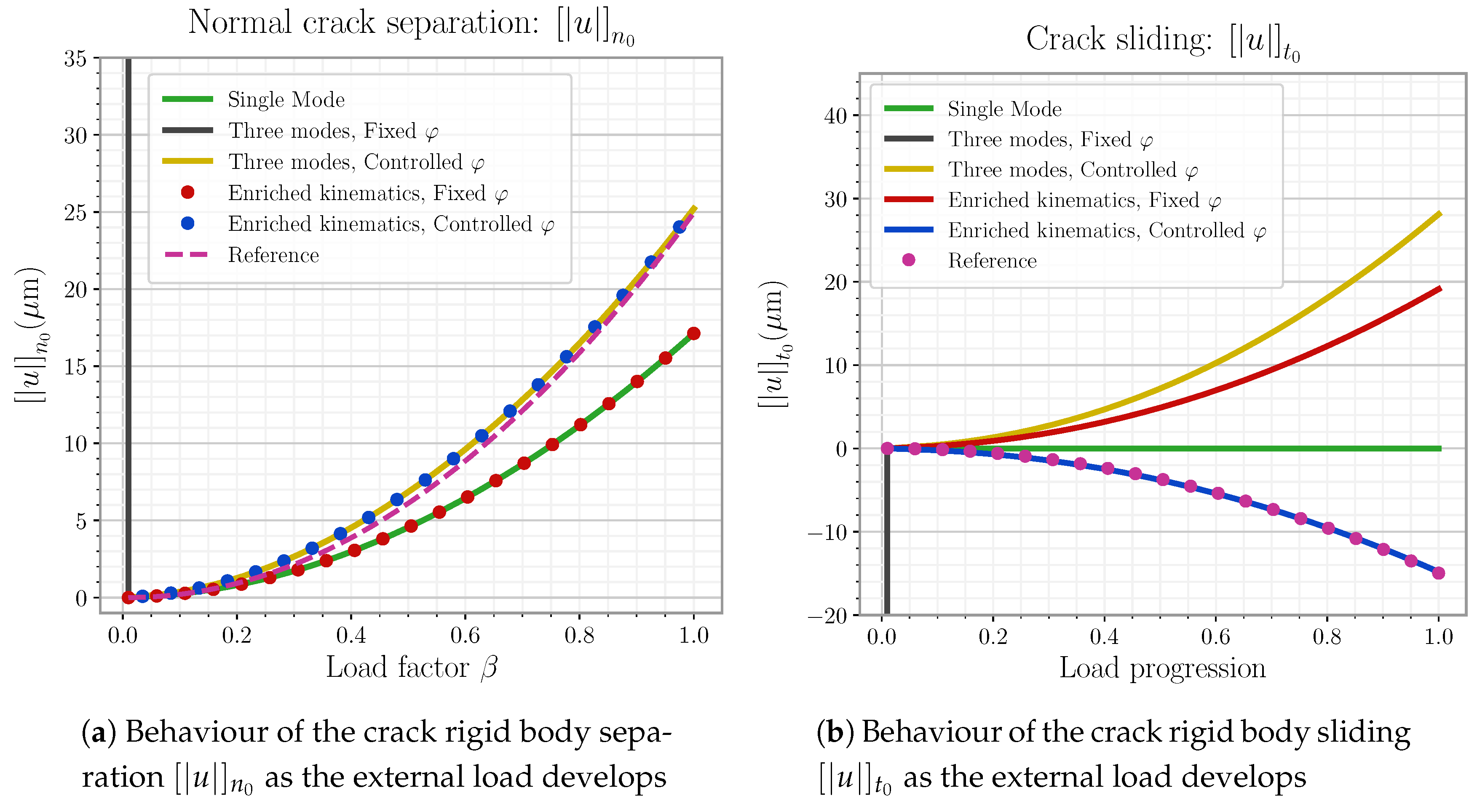
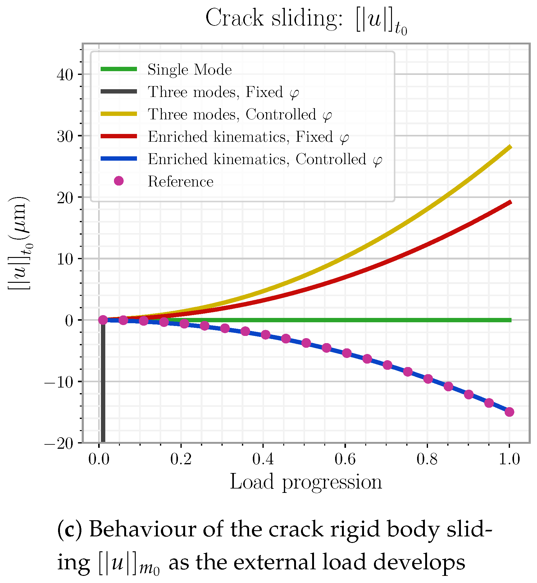
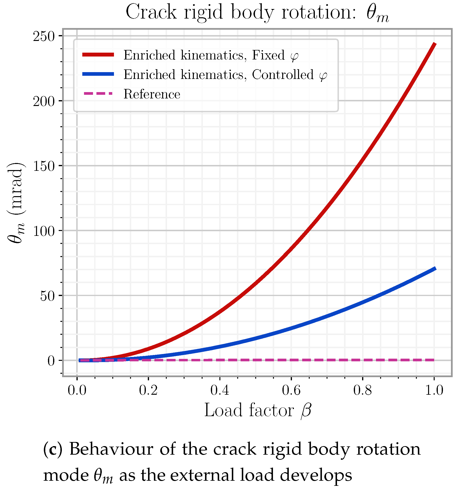
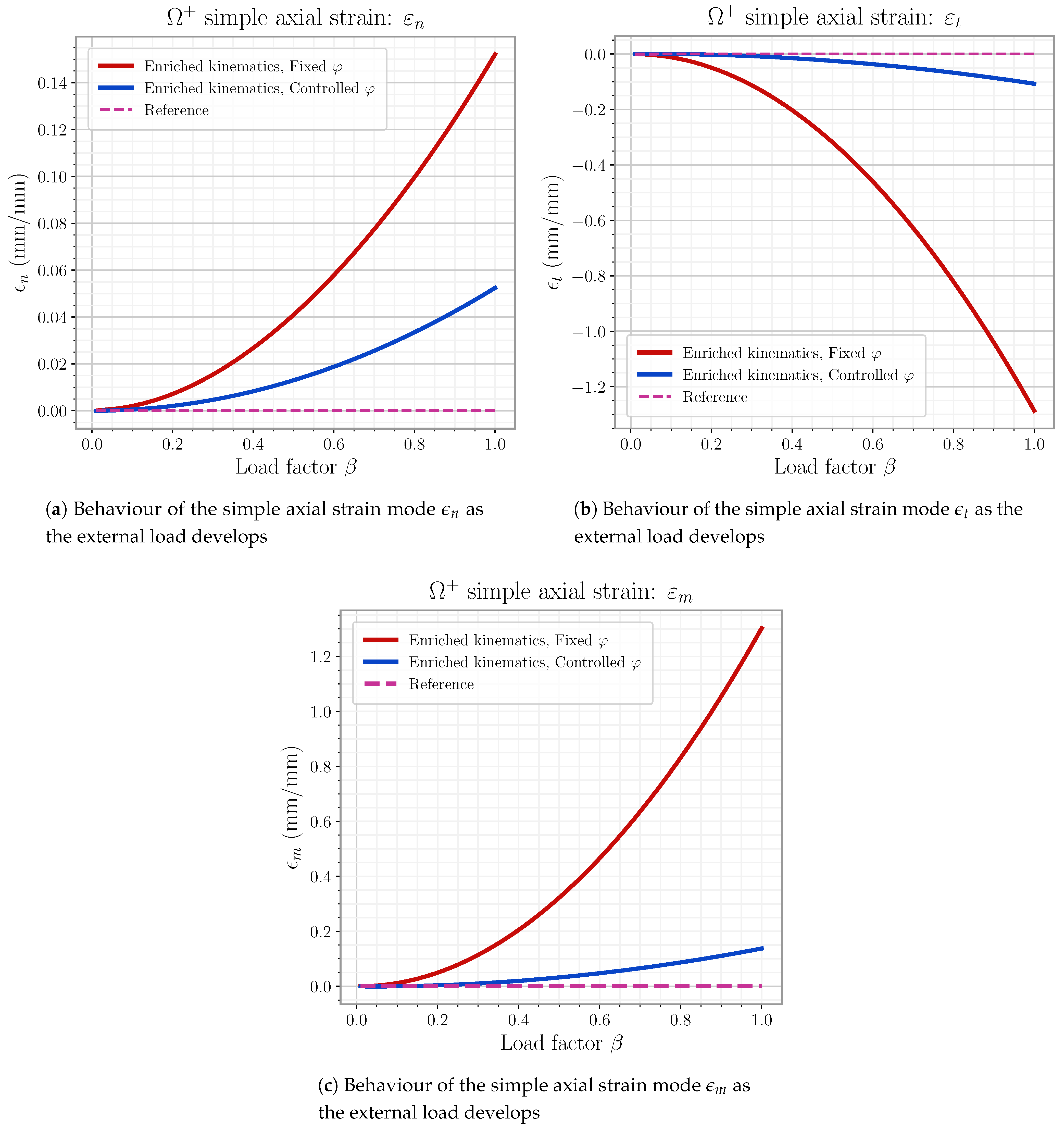
6.4.2. Kinematic Results
7. Conclusions
Author Contributions
Funding
Institutional Review Board Statement
Informed Consent Statement
Data Availability Statement
Acknowledgments
Conflicts of Interest
Abbreviations
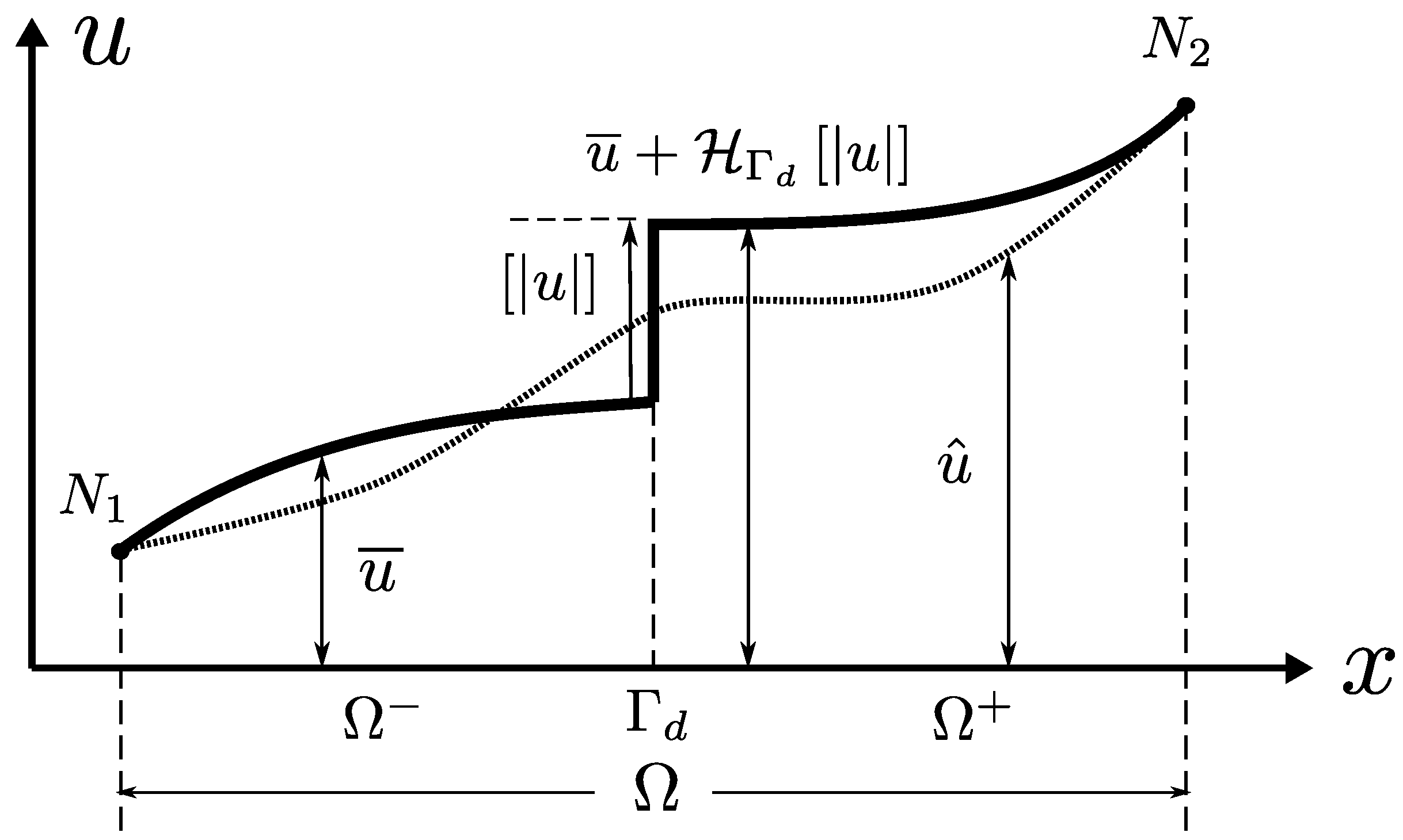
| Basic kinematics: | |
| Displacement field vector | |
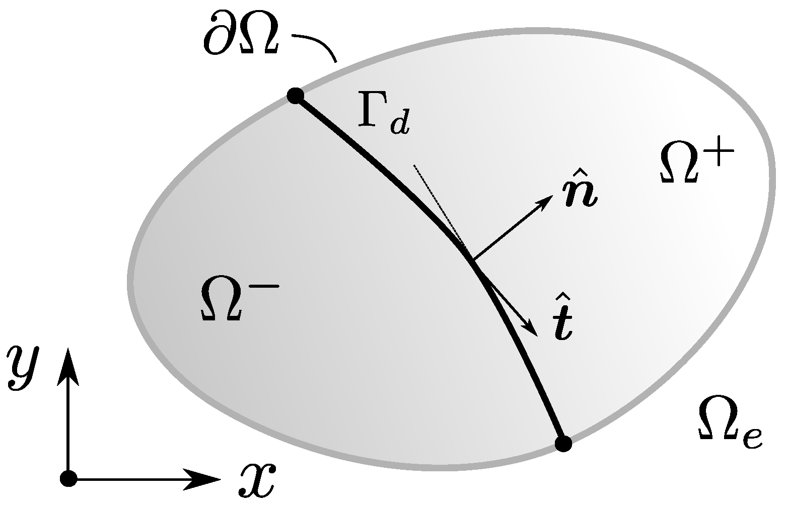
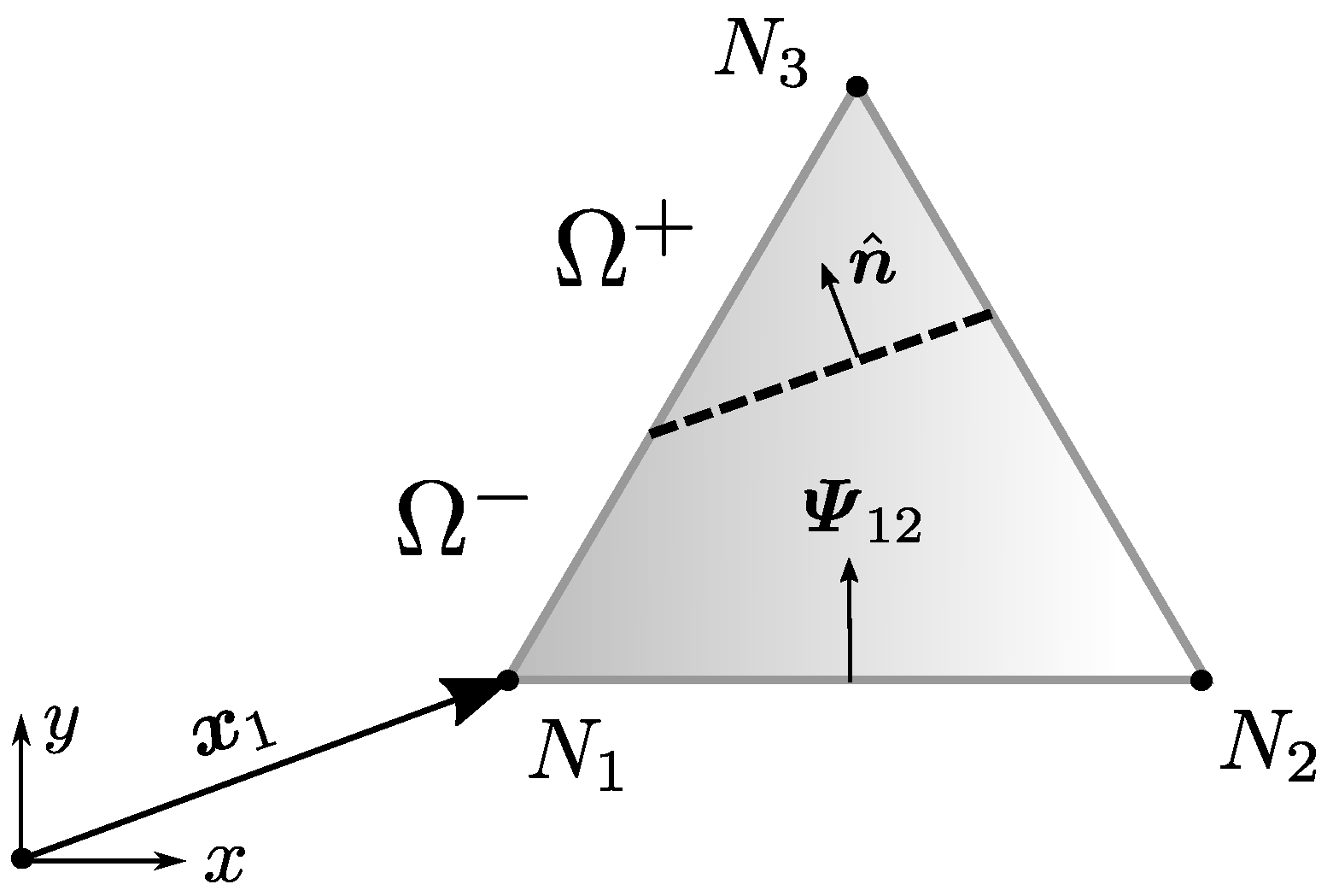
| Discontinuity (local fracture) surface | |
| “+” domain of the local fracture element partitions | |
| “−” domain of the local fracture element partitions | |
| Heaviside function having as a positional trigger | |
| Displacement jump vector | |
| Discontinuity-integrated displacement vector | |
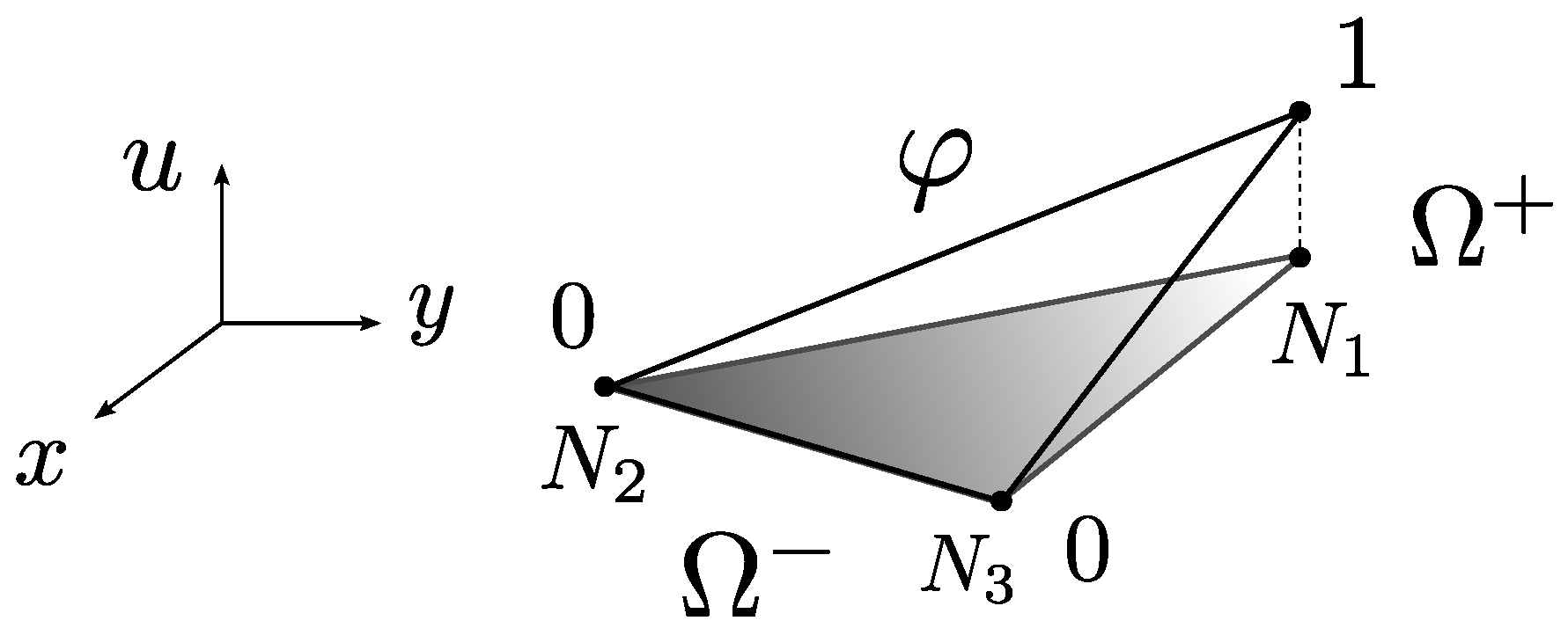
| Auxiliary function aiding the construction of , scalar version | |
| Compound, three-component definition of | |
| Dirac delta having as positional trigger | |
| Normal vector to the local fracture surface | |
| First parallel vector to the local fracture surface | |
| Second parallel vector to the local fracture surface | |
| Variational Analysis: | |
| Strain field vector (real) | |
| Strain field vector variation (virtual) | |
| Stress field vector (real) | |
| Stress field vector variation (virtual) | |
| Stress field calculated via constitutive relations based on real strains | |
| Linear elastic constitutive matrix | |
| Nodal displacement vector | |
| Nodal displacement vector variation (virtual) | |
| Displacement jump variation (virtual) | |
| Standard finite element displacement interpolation matrix | |
| Standard finite element strain interpolation matrix | |
| Strong discontinuity matrix operator | |
| Bounded section of the operator | |
| Unbounded section of the operator | |
| Strong discontinuity virtual matrix operator | |
| Bounded section of the operator | |
| Unbounded section of the operator | |
| Nodal stress vector | |
| Nodal stress vector variation (virtual) | |
| Real stress interpolation matrix | |
| Virtual stress interpolation matrix | |
| Projection matrix operator ( direction) | |
| Elemental volume | |
| Volume of the domain | |
| Volume of the domain | |
| Area of local fracture surface | |
| Local fracture surface traction vector | |
| Nodal displacement-driven part of surface traction vector | |
| Crack stiffness matrix, derived from projections on | |
| Displacement jump vector in the local fracture surface frame | |
| Advanced pathology analysis and new proposals: | |
| Rotation matrix onto the local frame | |
| Generalised fracture kinematics vector | |
| Fracture rigid body translation modes () | |
| Fracture rigid body rotation modes () | |
| Fracture simple axial strain modes () | |
| Generalised fracture kinematics interpolation matrix | |
| Compound strong discontinuity involving the operator | |
| Compound strong discontinuity involving the operator | |
| Volume-averaged operator through or | |
| Nodal displacement state associated with the fracture kinematic mode | |
| Binary indicator for element domains | |
| Polynomial coefficients for a compound definition | |
| Local coordinates in the fracture frame | |
| Fracture stiffness in terminal separation conditions for the j direction | |
| Projection matrix operator ( direction) | |
| Projection matrix operator ( direction) | |
| Crack stiffness matrix, derived from projections on | |
| Crack stiffness matrix, derived from projections on | |
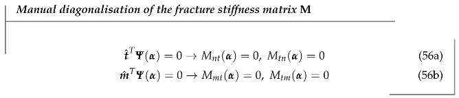
Appendix A. Derivation of an Explicit Crack Stiffness Matrix M
Appendix B. Analysis of φ Proposal by Wells
Appendix C. Detailed Description of φ Coefficients Linear System Building
References
- Ibrahimbegovic, A.; Wilson, E.L. A modified method of incompatible modes. Commun. Numer. Methods Eng. 1991, 7, 187–194. [Google Scholar] [CrossRef]
- Oliver, J.; Caicedo, M.; Roubin, E.; Huespe, A.; Hernández, J. Continuum approach to computational multiscale modeling of propagating fracture. Comput. Methods Appl. Mech. Eng. 2015, 294, 384–427. [Google Scholar] [CrossRef] [Green Version]
- Moës, N.; Dolbow, J.; Belytschko, T. A finite element method for crack growth without remeshing. Int. J. Numer. Methods Eng. 1999, 46, 131–150. [Google Scholar] [CrossRef]
- Oliver, J.; Huespe, A.; Sánchez, P. A comparative study on finite elements for capturing strong discontinuities: E-FEM vs. X-FEM. Comput. Methods Appl. Mech. Eng. 2006, 195, 4732–4752. [Google Scholar] [CrossRef]
- Tabiei, A.; Zhang, W. Evaluation of various numerical methods in LS-DYNA® for 3D Crack Propagation. In Proceedings of the Conference Proceedings 14th International LS-DYNA Users Conference, Detroit, MI, USA, 12–14 June 2016; Royal Dearborn Hotel and Convention Center: Detroit, MI, USA, 2016. [Google Scholar]
- Shi, J.; Lua, J.; Chen, L.; Chopp, D.; Sukumar, N. X-FEM for Abaqus (XFA) Toolkit for Automated Crack Onset and Growth Simulation: New Development, Validation, and Demonstration. In Proceedings of the Conference Proceedings 2009 SIMULIA Customer Conference, London, UK, 18–21 May 2009; The Brewery: London, UK, 2009. [Google Scholar]
- Weaver, C.M.; Rigg, P.A.; Cordes, J.A.; Haynes, A. XFEM Analyses of Critical Cracks in a Pressure Tap for a 40mm Gun Breech. In Proceedings of the Conference proceedings 2011 SIMULIA Customer Conference, Barcelona, Spain, 17–19 May 2011. [Google Scholar]
- Contrafatto, L.; Cuomo, M.; Tommaso, G.; Venti, D. Computational issues in the Finite Element with Embedded Discontinuity Method based on non-homogenous displacement jump. In Proceedings of the Conference proceedings Aimeta XXI, Torino, Italy, 17–20 September 2013. [Google Scholar] [CrossRef]
- Wells, G.N. Discontinuous Modelling of Strain Localisation and Failure. Ph.D. Thesis, Delft University of Technology, Delft, The Netherlands, 2001. [Google Scholar] [CrossRef]
- Oliver, J. Modelling strong discontinuities in solid mechanics via strain softening constitutive equations. Part 2: Numerical simulation. Int. J. Numer. Methods Eng. 1996, 39, 3601–3623. [Google Scholar] [CrossRef]
- Linder, C.; Armero, F. Finite elements with embedded strong discontinuities for the modeling of failure in solids. Int. J. Numer. Methods Eng. 2007, 72, 1391–1433. [Google Scholar] [CrossRef]
- Da Costa, D.D.; Alfaiate, J.; Sluys, L.; Júlio, E. A discrete strong discontinuity approach. Eng. Fract. Mech. 2009, 76, 1176–1201. [Google Scholar] [CrossRef] [Green Version]
- Dujc, J.; Brank, B.; Ibrahimbegovic, A.; Brancherie, D. An embedded crack model for failure analysis of concrete solids. Comput. Concr. 2010, 7. [Google Scholar] [CrossRef] [Green Version]
- Jirásek, M. Comparative study on finite elements with embedded cracks. Comput. Methods Appl. Mech. Eng. 2000, 188, 307–330. [Google Scholar] [CrossRef]
- Oliver, J. Modelling strong discontinuities in solid mechanics via strain softening constitutive equations. Part 1: Fundamentals. Int. J. Numer. Methods Eng. 1996, 39, 3575–3600. [Google Scholar] [CrossRef]
- Dvorkin, E.N.; Cuitiño, A.M.; Gioia, G. Finite elements with displacement interpolated embedded localization lines insensitive to mesh size and distortions. Int. J. Numer Methods Eng. 1990, 30, 541–564. [Google Scholar] [CrossRef]
- Simo, J.C.; Oliver, J.; Armero, F. An analysis of strong discontinuities induced by strain-softening in rate-independent inelastic solids. Comput. Mech. 1993, 12, 277–296. [Google Scholar] [CrossRef]
- Armero, F.; Garikipati, K. An analysis of strong discontinuities in multiplicative finite strain plasticity and their relation with the numerical simulation of strain localization in solids. Int. J. Solids Struct. 1996, 33, 2863–2885. [Google Scholar] [CrossRef]
- Oliver, J.; Huespe, A.E.; Blanco, S.; Hirnyj, S. On a finite element with embedded discontinuities for numerical modeling of fracture. In Proceedings of the 11th International Conference on Fracture ICF11, Torino, Italy, 20–25 March 2005; Curran Associates, Inc.: Nice, France, 2005; pp. 1229–1234. [Google Scholar]
- Simo, J.C.; Rifai, M.S. A class of mixed assumed strain methods and the method of incompatible modes. Int. J. Numer. Methods Eng. 1990, 29, 1595–1638. [Google Scholar] [CrossRef]
- Wells, G.; Sluys, L. Three-dimensional embedded discontinuity model for brittle fracture. Int. J. Solids Struct. 2001, 38, 897–913. [Google Scholar] [CrossRef]
- Roubin, E.; Vallade, A.; Benkemoun, N.; Colliat, J.B. Multi-scale failure of heterogeneous materials: A double kinematics enhancement for Embedded Finite Element Method. Int. J. Solids Struct. 2015, 52, 180–196. [Google Scholar] [CrossRef]
- Hauseux, P.; Roubin, E.; Colliat, J.B. The embedded finite element method (E-FEM) for multicracking of quasi-brittle materials. In Porous Rock Fracture Mechanics; Shojaei, A.K., Shao, J., Eds.; Woodhead Publishing: Cambridge, UK, 2017; pp. 177–196. [Google Scholar] [CrossRef]
- Stamati, O.; Roubin, E.; Andò, E.; Malecot, Y. Tensile failure of micro-concrete: From mechanical tests to FE meso-model with the help of X-ray tomography. Meccanica 2019, 54, 707–722. [Google Scholar] [CrossRef]
- Stamati, O. Impact of Meso-Scale Heterogeneities on the Mechanical Behaviour of Concrete: Insights from In-Situ X-ray Tomography and E-FEM Modelling. Ph.D. Thesis, Université Grenoble Alpes, Grenoble, France, 2020. [Google Scholar]
- Alfaiate, J.; Simone, A.; Sluys, L. Non-homogeneous displacement jumps in strong embedded discontinuities. Int. J. Solids Struct. 2003, 40, 5799–5817. [Google Scholar] [CrossRef]
- Dujc, J.; Brank, B.; Ibrahimbegovic, A. Quadrilateral finite element with embedded strong discontinuity for failure analysis of solids. Comput. Model. Eng. Sci. 2010, 69, 223–260. [Google Scholar] [CrossRef]
- Raina, A.; Linder, C. Modeling crack micro-branching using finite elements with embedded strong discontinuities. PAMM 2010, 10, 681–684. [Google Scholar] [CrossRef]
- Dias-da Costa, D.; Alfaiate, J.; Sluys, L.; Areias, P.; Júlio, E. An embedded formulation with conforming finite elements to capture strong discontinuities. Int. J. Numer. Methods Eng. 2013, 93, 224–244. [Google Scholar] [CrossRef]
- Brunton, S.; Kutz, J. Data-Driven Science and Engineering—Machine Learning, Dynamical Systems, and Control; Cambridge University Press: Cambridge, UK, 2019; pp. 3–46. [Google Scholar]
- The Sage Developers. SageMath, the Sage Mathematics Software System (Version 8.7). 2019. Available online: https://www.sagemath.org (accessed on 2 October 2020).
- Kluyver, T.; Ragan-Kelley, B.; Pérez, F.; Granger, B.; Bussonnier, M.; Frederic, J.; Kelley, K.; Hamrick, J.; Grout, J.; Corlay, S.; et al. Jupyter Notebooks—A publishing format for reproducible computational workflows. In Positioning and Power in Academic Publishing: Players, Agents and Agendas; Loizides, F., Scmidt, B., Eds.; IOS Press: Amsterdam, The Netherlands, 2016; pp. 87–90. [Google Scholar] [CrossRef]
- Hauseux, P. Propagation D’Incertitudes Paramétriques Dans Les Modèles Numériques en Mécanique Non Linéaire: Applications à des Problèmes D’excavation. Ph.D. Thesis, Université de Lille, Lille, France, 2015. [Google Scholar]
- Vallade, A. Modélisation Multi-échelles des Shales: Influence de la Microstructure sur les Propriétés Macroscopiques et le Processus de Fracturation. Ph.D. Thesis, Université de Lille, Lille, France, 2016. [Google Scholar]


Publisher’s Note: MDPI stays neutral with regard to jurisdictional claims in published maps and institutional affiliations. |
© 2021 by the authors. Licensee MDPI, Basel, Switzerland. This article is an open access article distributed under the terms and conditions of the Creative Commons Attribution (CC BY) license (https://creativecommons.org/licenses/by/4.0/).
Share and Cite
Ortega Laborin, A.; Roubin, E.; Malecot, Y.; Daudeville, L. General Consistency of Strong Discontinuity Kinematics in Embedded Finite Element Method (E-FEM) Formulations. Materials 2021, 14, 5640. https://doi.org/10.3390/ma14195640
Ortega Laborin A, Roubin E, Malecot Y, Daudeville L. General Consistency of Strong Discontinuity Kinematics in Embedded Finite Element Method (E-FEM) Formulations. Materials. 2021; 14(19):5640. https://doi.org/10.3390/ma14195640
Chicago/Turabian StyleOrtega Laborin, Alejandro, Emmanuel Roubin, Yann Malecot, and Laurent Daudeville. 2021. "General Consistency of Strong Discontinuity Kinematics in Embedded Finite Element Method (E-FEM) Formulations" Materials 14, no. 19: 5640. https://doi.org/10.3390/ma14195640
APA StyleOrtega Laborin, A., Roubin, E., Malecot, Y., & Daudeville, L. (2021). General Consistency of Strong Discontinuity Kinematics in Embedded Finite Element Method (E-FEM) Formulations. Materials, 14(19), 5640. https://doi.org/10.3390/ma14195640