
Artificial Intelligence Aided Design of Tissue Engineering Scaffolds Employing Virtual Tomography and 3D Convolutional Neural Networks


Abstract
:1. Introduction
2. Materials and Methods
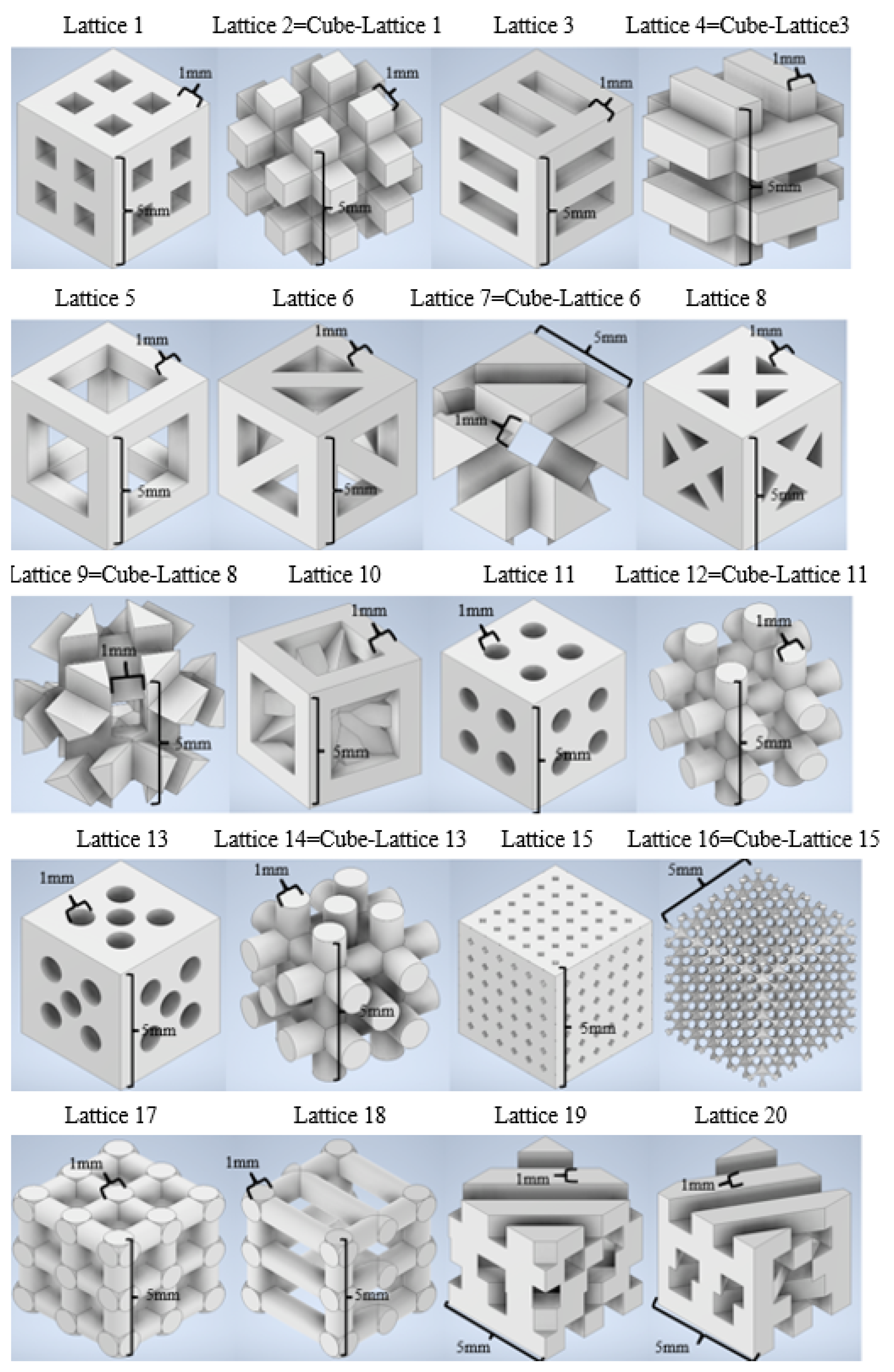
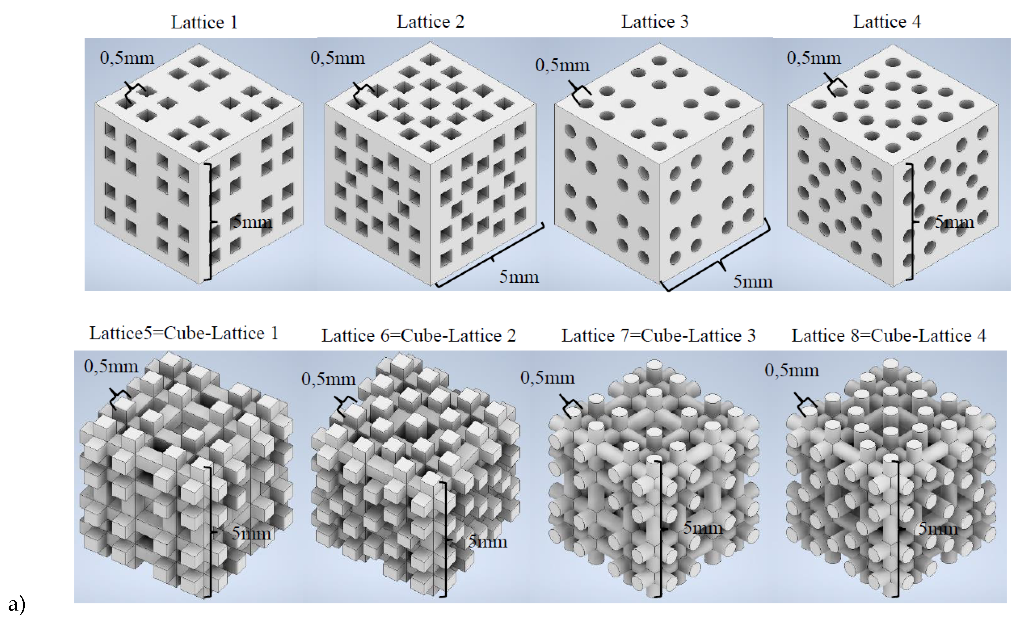
2.1. Creating a Library of Tissue Engineering Scaffolds with Well-Known Properties
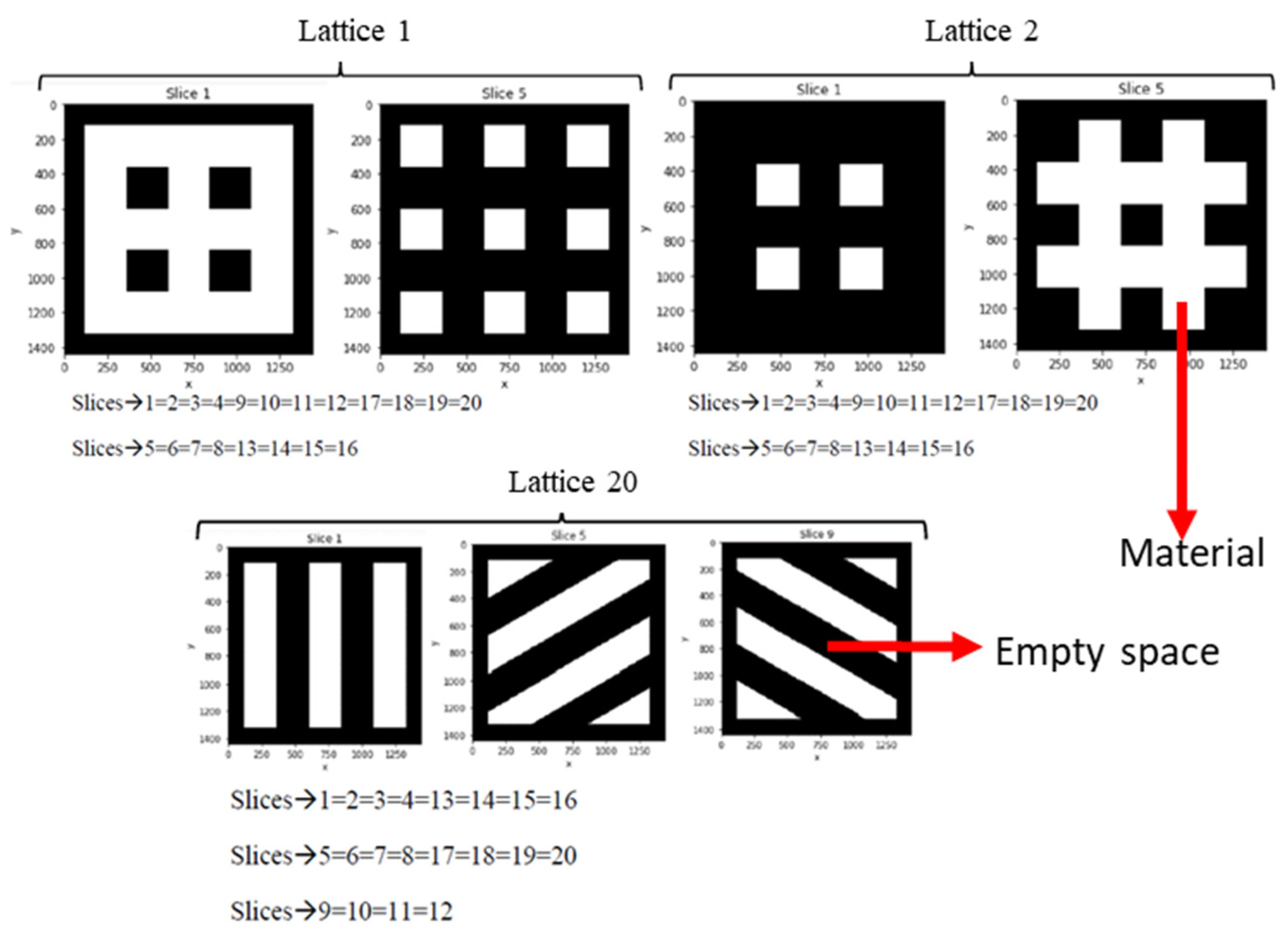
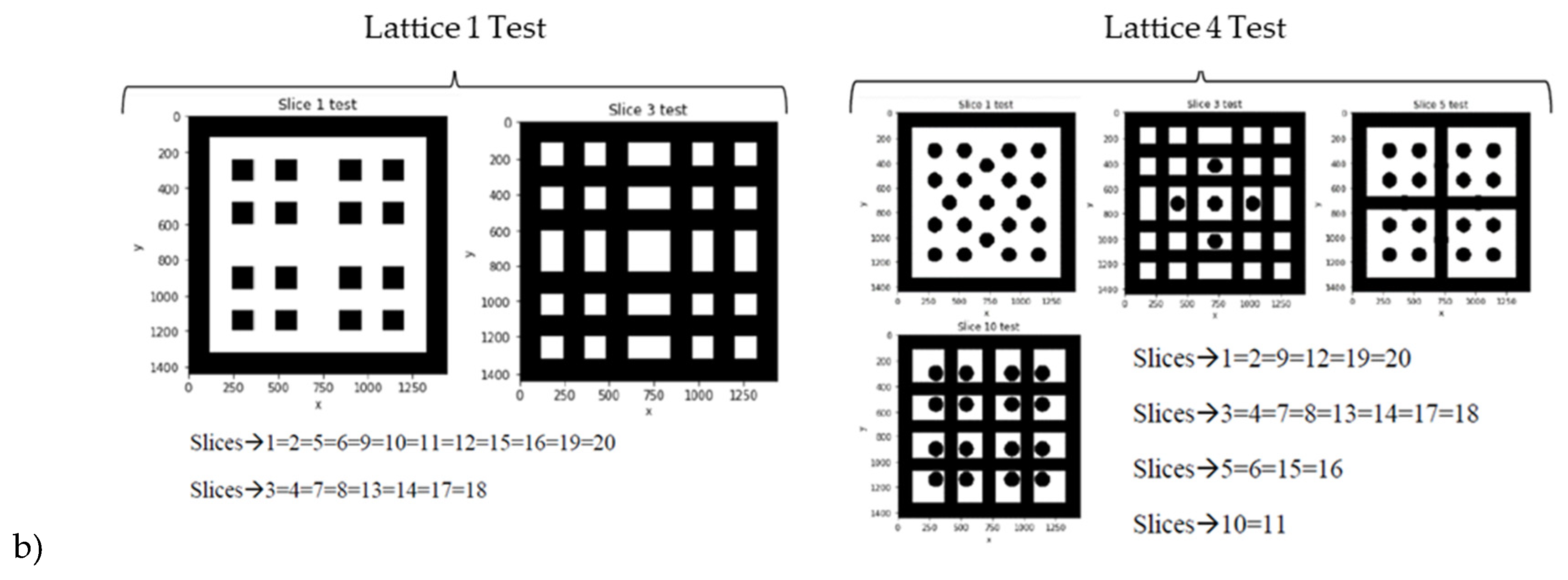
2.2. From 3D CAD Files to Digital Tomographies as Input for 3D CNNs
2.3. Structuring and Training 3D CNNs for Predicting Mechanical Properties

| Strategy | Number of Lattices Used | Number of Lattices Used for Training | Number of Lattices Used for Validation | Data Augmentation Strategy |
|---|---|---|---|---|
| 1st strategy | 20 | 14 random ones | 6 random ones | - |
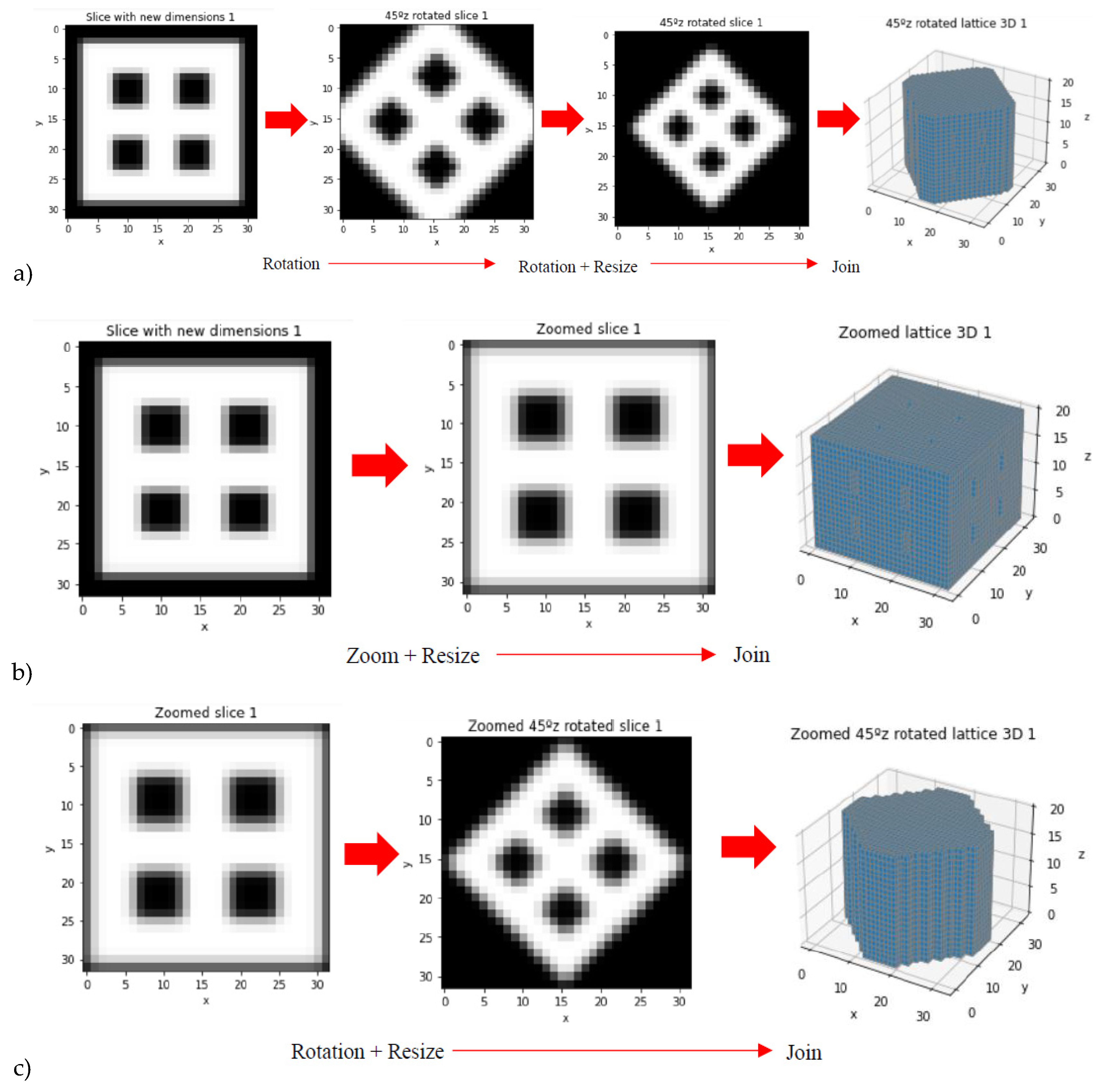
| 2nd strategy | 120 | 114 random ones | 6 random ones | Rotations around z-axis (15°, 30°, 45°, 60°, 75°) |
| 3rd strategy | 240 | 234 random ones | 6 random ones | Previous rotations plus zoomed-in lattices |
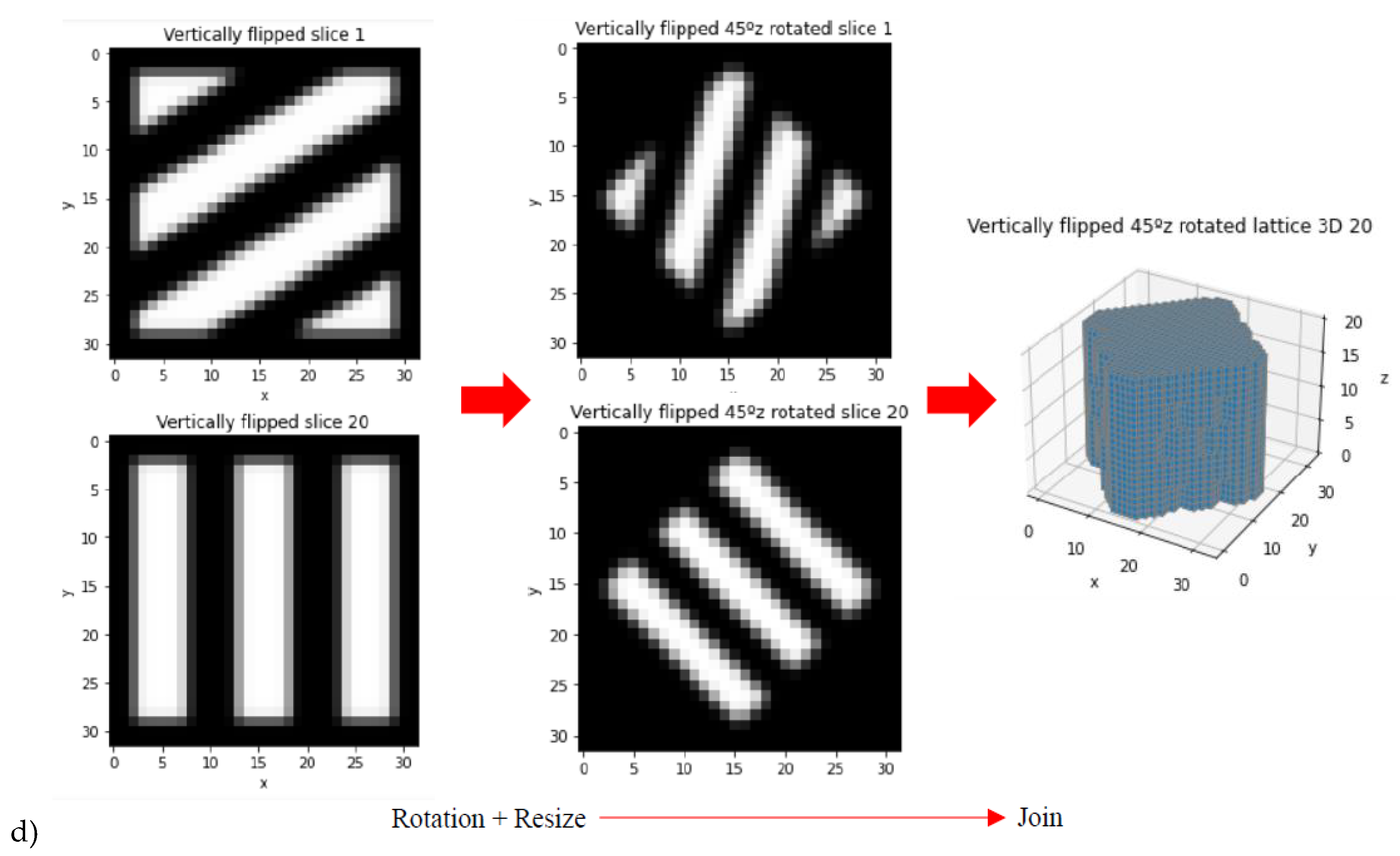
| 4th strategy | 360 | 354 random ones | 6 random ones | Previous rotations and zooms (240 lattices) plus vertical flips without zoom (120 lattices more) |
| 5th strategy | 480 | 474 random ones | 6 random ones | Addition of horizontal flips (120 lattices more) |
| 6th strategy | 680 | 674 random ones | 6 random ones | Addition of rotated initial lattices around x- and y-axes (15°, 30°, 45°, 60°, 75°, 200 lattices more) |
2.4. Testing and Validation of the Global Strategy
3. Results and Discussion
3.1. CAD Models, Digital Tomographies, and Training and Validation of 3D CNNs
3.2. Performance of the Structured and Trained 3D CNNs: Predictions vs. Real Performance
4. Challenges and Future Proposals
4.1. Potentials, Limitations, and Challenges of the Study
4.2. Future Research Proposals
5. Conclusions
Author Contributions
Funding
Institutional Review Board Statement
Informed Consent Statement
Data Availability Statement
Acknowledgments
Conflicts of Interest
Appendix A
| Lattice nº | Simulated Relative Porosity (%) | Predicted Relative Porosity (%) | Relative Porosity AE | Relative Porosity MAE | Simulated Rel. Elastic Modulus E_Relative (%) | Predicted Rel. Elastic Modulus E_Relative (%) | Rel. Elastic Modulus E_Relative AE | Rel. Elastic Modulus E_Relative MAE | Simulated Rel. Shear Modulus G_Relative (%) | Predicted Rel. Shear Modulus G_relative (%) | Rel. Shear Modulus G_Relative AE | Rel. Shear Modulus G_Relative MAE |
|---|---|---|---|---|---|---|---|---|---|---|---|---|
| 1st strategy | ||||||||||||
| Lattice 1 | 35.138 | −0.569 | 35.706 | 39.073 | 42.645 | 63.123 | 20.478 | 26.814 | 13.755 | 27.629 | 13.874 | 13.193 |
| Lattice 2 | 47.527 | −0.750 | 48.277 | 21.503 | 29.878 | 8.374 | 8.988 | 12.163 | 3.175 | |||
| Lattice 3 | 28.650 | −0.559 | 29.209 | 52.309 | 82.533 | 30.224 | 18.775 | 25.614 | 6.839 | |||
| Lattice 4 | 38.641 | −0.780 | 39.421 | 35.758 | 56.540 | 20.782 | 14.793 | 30.589 | 15.796 | |||
| Lattice 5 | 64.862 | 25.843 | 39.019 | 18.462 | −0.074 | 18.536 | 3.126 | 1.489 | 1.637 | |||
| Lattice 6 | 52.473 | −0.764 | 53.237 | 25.252 | 77.633 | 52.381 | 4.658 | 33.474 | 28.816 | |||
| Lattice 7 | 71.350 | 76.944 | 5.594 | 14.336 | −0.072 | 14.408 | 2.118 | 0.077 | 2.041 | |||
| Lattice 8 | 61.359 | −0.763 | 62.123 | 17.785 | 67.116 | 49.331 | 1.143 | 34.510 | 33.367 | |||
| 2nd strategy | ||||||||||||
| Lattice 1 | 35.138 | 12.707 | 22.431 | 18.476 | 42.645 | 62.542 | 19.897 | 18.926 | 13.755 | 24.392 | 10.638 | 9.263 |
| Lattice 2 | 47.527 | 57.088 | 9.561 | 21.503 | 4.106 | 17.397 | 8.988 | 4.646 | 4.342 | |||
| Lattice 3 | 28.650 | 29.877 | 1.226 | 52.309 | 77.738 | 25.429 | 18.775 | 29.877 | 11.102 | |||
| Lattice 4 | 38.641 | 38.019 | 0.622 | 35.758 | 24.999 | 10.759 | 14.793 | 13.045 | 1.749 | |||
| Lattice 5 | 64.862 | 49.150 | 15.713 | 18.462 | 19.016 | 0.554 | 3.126 | 7.370 | 4.243 | |||
| Lattice 6 | 52.473 | 7.153 | 45.320 | 25.252 | 71.796 | 46.544 | 4.658 | 27.718 | 23.060 | |||
| Lattice 7 | 71.350 | 53.194 | 18.155 | 14.336 | 17.750 | 3.414 | 2.118 | 6.110 | 3.992 | |||
| Lattice 8 | 61.359 | 26.582 | 34.777 | 17.785 | 45.202 | 27.417 | 1.143 | 16.120 | 14.977 | |||
| Lattice nº | Simulated Relative Porosity (%) | Predicted Relative Porosity (%) | Relative Porosity AE | Relative Porosity MAE | Simulated Rel. Elastic Modulus E_Relative (%) | Predicted Rel. Elastic Modulus E_Relative (%) | Rel. Elastic Modulus E_Relative AE | Rel. Elastic Modulus E_Relative MAE | Simulated Rel. Shear Modulus G_Relative (%) | Predicted Rel. Shear Modulus G_Relative (%) | Rel. Shear Modulus G_Relative AE | Rel. Shear Modulus G_Relative MAE |
|---|---|---|---|---|---|---|---|---|---|---|---|---|
| 3rd strategy | ||||||||||||
| Lattice 1 | 35.138 | 41.831 | 6.694 | 17.646 | 42.645 | 18.270 | 24.375 | 20.207 | 13.755 | 12.084 | 1.670 | 5.634 |
| Lattice 2 | 47.527 | 91.267 | 43.740 | 21.503 | −0.201 | 21.704 | 8.988 | −0.187 | 9.175 | |||
| Lattice 3 | 28.650 | 32.668 | 4.018 | 52.309 | 26.848 | 25.461 | 18.775 | 14.455 | 4.320 | |||
| Lattice 4 | 38.641 | 89.796 | 51.155 | 35.758 | −0.239 | 35.997 | 14.793 | −0.160 | 14.954 | |||
| Lattice 5 | 64.862 | 60.900 | 3.963 | 18.462 | −0.137 | 18.599 | 3.126 | −0.101 | 3.227 | |||
| Lattice 6 | 52.473 | 32.554 | 19.919 | 25.252 | 22.132 | 3.120 | 4.658 | 12.956 | 8.298 | |||
| Lattice 7 | 71.350 | 66.871 | 4.479 | 14.336 | −0.185 | 14.521 | 2.118 | −0.143 | 2.261 | |||
| Lattice 8 | 61.359 | 68.560 | 7.201 | 17.785 | −0.098 | 17.883 | 1.143 | −0.025 | 1.167 | |||
| 4th strategy | ||||||||||||
| Lattice 1 | 35.138 | 27.745 | 7.393 | 14.577 | 42.645 | 45.714 | 3.069 | 12.108 | 13.755 | 18.809 | 5.054 | 6.823 |
| Lattice 2 | 47.527 | 86.467 | 38.940 | 21.503 | 0.292 | 21.211 | 8.988 | −0.003 | 8.991 | |||
| Lattice 3 | 28.650 | 17.930 | 10.720 | 52.309 | 60.546 | 8.237 | 18.775 | 24.280 | 5.505 | |||
| Lattice 4 | 38.641 | 65.936 | 27.296 | 35.758 | 16.456 | 19.303 | 14.793 | 6.952 | 7.841 | |||
| Lattice 5 | 64.862 | 61.508 | 3.354 | 18.462 | 22.591 | 4.130 | 3.126 | 7.012 | 3.886 | |||
| Lattice 6 | 52.473 | 26.997 | 25.476 | 25.252 | 55.402 | 30.150 | 4.658 | 20.239 | 15.581 | |||
| Lattice 7 | 71.350 | 68.602 | 2.748 | 14.336 | 21.723 | 7.387 | 2.118 | 4.622 | 2.503 | |||
| Lattice 8 | 61.359 | 62.052 | 0.693 | 17.785 | 21.164 | 3.378 | 1.143 | 6.365 | 5.222 | |||
| Lattice nº | Simulated Relative Porosity (%) | Predicted Relative Porosity (%) | Relative Porosity AE | Relative Porosity MAE | Simulated Rel. Elastic Modulus E_Relative (%) | Predicted Rel. Elastic Modulus E_Relative (%) | Rel. Elastic Modulus E_Relative AE | Rel. Elastic Modulus E_Relative MAE | Simulated Rel. Shear Modulus G_Relative (%) | Predicted Rel. Shear Modulus G_Relative (%) | Rel. Shear Modulus G_Relative AE | Rel. Shear Modulus G_Relative MAE |
|---|---|---|---|---|---|---|---|---|---|---|---|---|
| 5th strategy | ||||||||||||
| Lattice 1 | 35.138 | 35.598 | 0.460 | 15.496 | 42.645 | 42.575 | 0.070 | 18.713 | 13.755 | 13.167 | 0.588 | 9.289 |
| Lattice 2 | 47.527 | 47.341 | 0.187 | 21.503 | 29.543 | 8.040 | 8.988 | 17.428 | 8.440 | |||
| Lattice 3 | 28.650 | 33.927 | 5.276 | 52.309 | 43.521 | 8.789 | 18.775 | 14.347 | 4.428 | |||
| Lattice 4 | 38.641 | 31.366 | 7.275 | 35.758 | 43.336 | 7.578 | 14.793 | 22.453 | 7.660 | |||
| Lattice 5 | 64.862 | 44.621 | 20.242 | 18.462 | 35.414 | 16.952 | 3.126 | 7.862 | 4.736 | |||
| Lattice 6 | 52.473 | 21.655 | 30.818 | 25.252 | 67.866 | 42.614 | 4.658 | 25.450 | 20.793 | |||
| Lattice 7 | 71.350 | 47.203 | 24.147 | 14.336 | 36.286 | 21.950 | 2.118 | 7.237 | 5.118 | |||
| Lattice 8 | 61.359 | 25.800 | 35.559 | 17.785 | 61.499 | 43.714 | 1.143 | 23.696 | 22.553 | |||
| 6th strategy | ||||||||||||
| Lattice 1 | 35.138 | 24.881 | 10.257 | 7.665 | 42.645 | 33.416 | 9.229 | 10.264 | 13.755 | 18.620 | 4.865 | 3.242 |
| Lattice 2 | 47.527 | 57.971 | 10.444 | 21.503 | 18.641 | 2.862 | 8.988 | 7.243 | 1.745 | |||
| Lattice 3 | 28.650 | 24.990 | 3.660 | 52.309 | 33.358 | 18.951 | 18.775 | 18.512 | 0.263 | |||
| Lattice 4 | 38.641 | 36.310 | 2.331 | 35.758 | 26.531 | 9.227 | 14.793 | 14.152 | 0.641 | |||
| Lattice 5 | 64.862 | 62.012 | 2.850 | 18.462 | 5.179 | 13.283 | 3.126 | 3.943 | 0.817 | |||
| Lattice 6 | 52.473 | 34.515 | 17.957 | 25.252 | 25.039 | 0.213 | 4.658 | 13.551 | 8.893 | |||
| Lattice 7 | 71.350 | 79.106 | 7.756 | 14.336 | 3.789 | 10.547 | 2.118 | 0.402 | 1.717 | |||
| Lattice 8 | 61.359 | 67.421 | 6.062 | 17.785 | −0.013 | 17.799 | 1.143 | 8.139 | 6.997 | |||
References
- Interagency Materials Genome Initiative Web Portal. Available online: https://www.mgi.gov (accessed on 23 June 2021).
- NIST Gateway to Materials Genome Information. Available online: https://mgi.nist.gov/ (accessed on 23 June 2021).
- Liu, Z.H. Perspective on Materials Genome®. Chin. Sci. Bull. 2014, 59, 1619–1623. [Google Scholar] [CrossRef]
- Qian, C.; Siler, T.; Ozin, G.A. Exploring the possibilities and limitations of a nanomaterials genome. Small 2015, 11, 64–69. [Google Scholar] [CrossRef]
- Raccuglia, P.; Elbert, K.C.; Adler, P.D.F.; Falk, C.; Wenny, M.B.; Mollo, A.; Zeller, M.; Friedler, S.A.; Schrier, J. Machine-learning-assisted materials discovery using failed experiments. Nature 2016, 533, 73–76. [Google Scholar] [CrossRef]
- Lu, W.; Xiao, R.; Yang, J.; Li, H.; Zhang, W. Data-mining aided materials discovery and optimization. J. Mater. 2017, 3, 191–201. [Google Scholar] [CrossRef]
- Winkler, D.A. Biomimetic molecular design tools that learn, evolve, and adapt. Beilstein J. Org. Chem. 2017, 13, 1288–1302. [Google Scholar] [CrossRef] [Green Version]
- Jose, R.; Ramakrishna, S. Materials 4.0: Materials big data enabled materials discovery. Appl. Mater. Today 2018, 10, 127–132. [Google Scholar] [CrossRef]
- Santos, I.; Nieves, J.; Penya, Y.K.; Bringas, P. Machine-learning-based mechanical properties prediction in foundry production. In Proceedings of the ICCAS-SICE 2009—ICROS-SICE International Joint Conference 2009, Fukuoka, Japan, 18–21 August 2009; pp. 4536–4541. [Google Scholar]
- Merayo, D.; Rodríguez-Prieto, Á.; Camacho, A. Prediction of physical and mechanical properties for metallic materials selection using big data and artificial neural networks. IEEE Access 2017, 20, 1–9. [Google Scholar] [CrossRef]
- Díaz Lantada, A.; Franco-Martínez, F.; Hengsbach, S.; Rupp, F.; Thelen, R.; Bade, K. Artificial intelligence aided design of microtextured surfaces: Application to controlling wettability. Nanomaterials 2020, 10, 2287. [Google Scholar] [CrossRef] [PubMed]
- Jiao, P.; Alavi, A.H. Artificial intelligence-enabled smart mechanical metamaterials: Advent and future trends. Int. Mater. Rev. 2021, 66, 365–393. [Google Scholar] [CrossRef]
- Bonfanti, S.; Guerra, R.; Font-Clos, F.; Rayneau-Kirkhope, D.; Zapperi, S. Automatic design of mechanical metamaterial actuators. Nat. Commun. 2020, 11, 4162. [Google Scholar] [CrossRef] [PubMed]
- Langer, R.; Vacanti, J.P. Tissue engineering. Science 1993, 260, 920–926. [Google Scholar] [CrossRef] [Green Version]
- Khademhosseini, A.; Vacanti, J.P.; Langer, R. Progress in tissue engineering. Sci. Am. 2009, 300, 64–71. [Google Scholar] [CrossRef] [PubMed]
- Boccaccio, A.; Ballini, A.; Pappalettere, C.; Tullo, D.; Cantore, S.; Desiate, A. Finite element method (FEM), mechanobiology and biomimetic scaffolds in bone tissue engineering. Int. J. Biol. Sci. 2011, 7, 112–132. [Google Scholar] [CrossRef] [PubMed]
- Egan, P.F.; Gonella, V.C.; Engensperger, M.; Ferguson, S.J.; Shea, K. Computationally designed lattices with tuned properties for tissue engineering using 3D printing. PLoS ONE 2017, 12, e0182902. [Google Scholar]
- Conev, A.; Litsa, E.E.; Perez, M.R.; Diba, M.; Mikos, A.G.; Kavraki, L.E. Machine learning-guided three-dimensional printing of tissue engineering scaffolds. Tissue Eng. Part A 2020, 26, 1359–1368. [Google Scholar] [CrossRef] [PubMed]
- Xu, J.; Ge, H.; Zhou, X.; Yan, J.; Chi, Q.; Zhang, Z. Prediction of vascular tissue engineering results with artificial neural networks. J. Biomed. Inform. 2005, 38, 417–421. [Google Scholar] [CrossRef] [Green Version]
- Sujeeun, L.Y.; Goonoo, N.; Ramphul, H.; Chummun, I.; Gimié, F.; Baichoo, S.; Bhaw-Luximon, A. Correlating in vitro performance with physico-chemical characteristics of nanofibrous scaffolds for skin tissue engineering using supervised machine learning algorithms. R. Soc. Open Sci. 2020, 7, 201293. [Google Scholar] [CrossRef] [PubMed]
- Rabbani, A.; Babaei, M.; Shams, R.; Wang, Y.D.; Chung, T. DeePore: A deep learning workflow for rapid and comprehensive characterization of porous materials. Adv. Water Resour. 2020, 146, 103787. [Google Scholar] [CrossRef]
- Serj, M.F.; Lavi, B.; Hoff, G.; Valls, D.P. A deep convolutional neural network for lung cancer diagnostic. arXiv 2018, arXiv:1804.08170. [Google Scholar]
- Bassi, P.R.A.S.; Attux, R. A deep convolutional neural network for COVID-19 detection using chest X-rays. Res. Biomed. Eng. 2021, 1–10. [Google Scholar] [CrossRef]
- Ghaderzadeh, M.; Asadi, F.; Jafari, R.; Bashash, D.; Abolghasemi, H.; Aria, M. Deep convolutional neural network-based computer-aided detection system for COVID-19 using multiple lung scans: Design and Implementation Study. J. Med. Internet Res. 2021, 23, e27468. [Google Scholar] [CrossRef] [PubMed]
- García, I.E.G. Desarrollo de una red Neuronal Convolucional Volumétrica para la Síntesis de Imagen en Resonancia Magnética Nuclear Cerebral. Ph.D. Thesis, Universidad Politécnica de Valencia, Valencia, Spain, 2019. [Google Scholar]
- La librería Numpy. Aprende con Alf. Available online: https://aprendeconalf.es/docencia/python/manual/numpy/ (accessed on 23 June 2021).
- Matplotlib: Python Plotting—Matplotlib 3.4.2 Documentation. 2021. Available online: https://matplotlib.org/ (accessed on 23 June 2021).
- Scikit-Learn: Machine Learning in Python—Scikit-Learn 0.24.2 Documentation. Available online: https://scikit-learn.org/stable/ (accessed on 23 June 2021).
- Santos, P.G.D.L. Introducción a Scikit-Image, Procesamiento de Imágenes en Python. 2016. Available online: https://numython.github.io/posts/2016/01/introduccion-scikit-image-procesamiento/ (accessed on 23 June 2021).
- TensorFlow. Available online: https://www.tensorflow.org/?hl=es-419 (accessed on 23 June 2021).
- Keras: The Python Deep Learning API. Available online: https://keras.io/guides/ (accessed on 23 June 2021).
- Keras Batch Normalization Layer. Available online: https://keras.io/api/layers/normalization_layers/batch_normalization/ (accessed on 23 June 2021).
- Brownlee, J. A gentle introduction to batch normalization for deep neural networks. In Machine Learning Mastery; Machine Learning Mastery: San Juan, Puerto Rico, 2019; Available online: https://machinelearningmastery.com/batch-normalization-for-training-of-deep-neural-networks/ (accessed on 23 June 2021).
- Keras Dropout Layer. Available online: https://keras.io/api/layers/regularization_layers/dropout/ (accessed on 23 June 2021).
- Zunair, H. 3D Image Classification from CT Scans. Available online: https://keras.io/examples/vision/3D_image_classification/ (accessed on 23 June 2021).
- Chan, C.H.M. Step by Step Implementation: 3D Convolutional Neural Network in Keras. In Towards Data Science; 2020; Available online: https://towardsdatascience.com/about (accessed on 26 July 2021).
- Alwattar, T.A.; Mian, A. Development of an Elastic Material Model for BCC Lattice Cell Structures Using Finite Element Analysis and Neural Networks Approaches. J. Compos. Sci. 2019, 3, 33. [Google Scholar] [CrossRef] [Green Version]
- Jafari Chashmi, M.; Fathi, A.; Shirzad, M.; Jafari-Talookolaei, R.-A.; Bodaghi, M.; Rabiee, S.M. Design and Analysis of Porous Functionally Graded Femoral Prostheses with Improved Stress Shielding. Designs 2020, 4, 12. [Google Scholar] [CrossRef]
- Sinitskiy, A.V.; Pande, V. Deep Neural Network Computes Electron Densities and Energies of a Large Set of Organic Molecules Faster than Density Functional Theory (DFT). arXiv 2018, arXiv:1809.02723. [Google Scholar]


| Lattice nº | Relative Porosity (%) | Relative Compression Modulus E_Relative (%) | Relative Shear Modulus G_Relative (%) |
|---|---|---|---|
| Lattice 1 | 35.2000 | 39.5401 | 13.0767 |
| Lattice 2 | 64.8000 | 18.5385 | 3.1629 |
| Lattice 3 | 48.0000 | 35.8848 | 5.9301 |
| Lattice 4 | 52.0000 | 30.0935 | 6.1656 |
| Lattice 5 | 64.8000 | 7.9094 | 2.0723 |
| Lattice 6 | 40.0864 | 8.8467 | 9.8194 |
| Lattice 7 | 59.9136 | 8.1076 | 3.4133 |
| Lattice 8 | 22.7736 | 29.9924 | 19.2402 |
| Lattice 9 | 77.2264 | 10.4106 | 0.9591 |
| Lattice 10 | 42.8672 | 21.1969 | 12.3903 |
| Lattice 11 | 28.6480 | 48.9160 | 18.4019 |
| Lattice 12 | 71.3520 | 14.3817 | 2.1877 |
| Lattice 13 | 36.9416 | 25.2379 | 14.4458 |
| Lattice 14 | 63.0584 | 18.2058 | 2.43572 |
| Lattice 15 | 6.31440 | 88.0836 | 33.2377 |
| Lattice 16 | 93.6864 | 1.4064 | 0.0704 |
| Lattice 17 | 45.7240 | 29.0857 | 11.1030 |
| Lattice 18 | 57.0864 | 26.7598 | 4.6127 |
| Lattice 19 | 45.3984 | 10.3383 | 6.9349 |
| Lattice 20 | 45.1312 | 20.6479 | 7.1886 |
| Lattice nº | Relative Porosity (%) | Relative Compression Modulus E_Relative (%) | Relative Shear Modulus G_Relative (%) |
|---|---|---|---|
| New Lattice 1 | 35.1376 | 42.6450 | 13.7545 |
| New Lattice 2 | 47.5272 | 21.5032 | 8.9878 |
| New Lattice 3 | 28.6504 | 52.3093 | 18.7747 |
| New Lattice 4 | 38.6408 | 35.7584 | 14.7934 |
| New Lattice 5 | 64.8624 | 18.4618 | 3.1262 |
| New Lattice 6 | 52.4728 | 25.2521 | 4.6577 |
| New Lattice 7 | 71.3496 | 14.3355 | 2.1183 |
| New Lattice 8 | 61.3592 | 17.7851 | 1.1427 |
| Strategy | Relative Porosity MAE | Relative Elastic Modulus MAE | Relative Shear Modulus MAE | Strategy Global MAE |
|---|---|---|---|---|
| 1st strategy | 39.073 | 26.814 | 13.193 | 26.360 |
| 2nd strategy | 18.476 | 18.926 | 9.263 | 15.555 |
| 3rd strategy | 17.646 | 20.207 | 5.634 | 14.496 |
| 4th strategy | 14.577 | 12.108 | 6.823 | 11.169 |
| 5th strategy | 15.496 | 18.713 | 9.289 | 14.500 |
| 6th strategy | 7.665 | 10.264 | 3.242 | 7.057 |
Publisher’s Note: MDPI stays neutral with regard to jurisdictional claims in published maps and institutional affiliations. |
© 2021 by the authors. Licensee MDPI, Basel, Switzerland. This article is an open access article distributed under the terms and conditions of the Creative Commons Attribution (CC BY) license (https://creativecommons.org/licenses/by/4.0/).
Share and Cite
Bermejillo Barrera, M.D.; Franco-Martínez, F.; Díaz Lantada, A. Artificial Intelligence Aided Design of Tissue Engineering Scaffolds Employing Virtual Tomography and 3D Convolutional Neural Networks. Materials 2021, 14, 5278. https://doi.org/10.3390/ma14185278
Bermejillo Barrera MD, Franco-Martínez F, Díaz Lantada A. Artificial Intelligence Aided Design of Tissue Engineering Scaffolds Employing Virtual Tomography and 3D Convolutional Neural Networks. Materials. 2021; 14(18):5278. https://doi.org/10.3390/ma14185278
Chicago/Turabian StyleBermejillo Barrera, María Dolores, Francisco Franco-Martínez, and Andrés Díaz Lantada. 2021. "Artificial Intelligence Aided Design of Tissue Engineering Scaffolds Employing Virtual Tomography and 3D Convolutional Neural Networks" Materials 14, no. 18: 5278. https://doi.org/10.3390/ma14185278
APA StyleBermejillo Barrera, M. D., Franco-Martínez, F., & Díaz Lantada, A. (2021). Artificial Intelligence Aided Design of Tissue Engineering Scaffolds Employing Virtual Tomography and 3D Convolutional Neural Networks. Materials, 14(18), 5278. https://doi.org/10.3390/ma14185278