Mass Transfer Principles in Column Percolation Tests: Initial Conditions and Tailing in Heterogeneous Materials

Abstract

Initial conditions (pre-equilibrium or after the first flooding of the column), mass transfer mechanisms and sample composition (heterogeneity) have a strong impact on leaching of less and strongly sorbing compounds in column percolation tests. Mechanistic models as used in this study provide the necessary insight to understand the complexity of column leaching tests especially when heterogeneous samples are concerned. By means of numerical experiments, we illustrate the initial concentration distribution inside the column after the first flooding and how this impacts leaching concentrations. Steep concentration gradients close to the outlet of the column have to be expected for small distribution coefficients ($K_d<1$ L kg⁻¹) and longitudinal dispersion leads to smaller initial concentrations than expected under equilibrium conditions. In order to elucidate the impact of different mass transfer mechanisms, film diffusion across an external aqueous boundary layer (first order kinetics, FD) and intraparticle pore diffusion (IPD) are considered. The results show that IPD results in slow desorption kinetics due to retarded transport within the tortuous intragranular pores. Non-linear sorption has not much of an effect if compared to $K_d$ values calculated for the appropriate concentration range (e.g., the initial equilibrium concentration). Sample heterogeneity in terms of grain size and different fractions of sorptive particles in the sample have a strong impact on leaching curves. A small fraction (<1%) of strongly sorbing particles (high $K_d$) carrying the contaminant may lead to very slow desorption rates (because of less surface area)—especially if mass release is limited by IPD—and thus non-equilibrium. In contrast, mixtures of less sorbing fine material (“labile” contamination with low $K_d$), with a small fraction of coarse particles carrying the contaminant leads to leaching close to or at equilibrium showing a step-wise concentration decline in the column effluent.

1. Introduction

Leaching tests are widely used for the determination of contaminant release rates from soils [1,2,3,4], recycling materials [5,6,7,8,9,10,11], construction products [12,13,14,15,16], radioactive and other waste materials [17,18]. Compared to traditional batch shaking tests, column tests are preferred for assessing the risk of release of potential pollutants into groundwater or surface waters because they are closer to natural conditions [19,20]. Different mechanisms controlling desorption kinetics may result in complex leaching behaviors. While initially the observed column effluent concentration often reflects equilibrium conditions between the solid phase (incl. intraparticle pores) and the mobile aqueous phase [21,22], the concentrations decrease and often an extended tailing is observed due to slow desorption processes such as intraparticle diffusion [23,24,25].

Although most leaching test procedures aim at equilibrium conditions in the column before the leaching starts, the true concentration distribution before the start of the percolation depends not only on the test procedure (contact time, pre-equilibration time, flow velocity during first flooding) but also on the properties of both the solid material and the pollutant of interest [26]. Equilibration and long-term leaching are further complicated if the test sample consists of a heterogeneous mixture of different material types and grain sizes [26,27,28], which is the common case if waste materials such as demolition waste or soils are tested.

Finkel and Grathwohl (2017) evaluated the role of initial conditions for column leaching tests with intraparticle pore diffusion models by comparing the hypothetical scenarios, a perfectly equilibrated column vs. a column that wasn’t equilibrated at all [26]. They could show that in many practical cases, peak and cumulative leachate concentrations are rather independent of the initial conditions. However, if release kinetics are slow due to large grain size or small intragranular porosity, the sensitivity to initial conditions is relevant, in particular for initial peak and early cumulative leachate concentrations.

The shortcomings of all previous studies [26,29,30], is that only uniform initial concentrations in the columns were considered in the leaching models. However, due to the specific conditions during the flooding of the column filled with initially dry material, the true initial conditions at the start of the leaching test may considerably deviate from this ideal, i.e., uniform distribution.

Against this background, the objectives of this study are (i) to illustrate the possibly non-uniform initial conditions that may be achieved after the first flooding of the column, (ii) to show the impact of these initial conditions on the temporal development of the effluent concentrations, and (iii) to investigate how heterogeneous mixtures of particles having different properties affect both the initial conditions in the column and the leaching of the solutes. To achieve that, we used numerical solutions for flow and transport in a column coupled to two kinetic models: (i) solute diffusion through an aqueous boundary layer and (ii) intraparticle pore diffusion. The implementation of the numerical models is described in detail in the appendices.

2. Theory and Background

2.1. Local Equilibrium: The Advection—Dispersion Equation

In order to facilitate the understanding of mass transfer-limited cases of contaminant release in a column, we briefly introduce the equilibrium case for which the advection-dispersion model is commonly used:

$$\frac{\partial }{\partial t}\left(n{C}_w+{\rho }_b{C}_s\right)+\frac{\partial }{\partial x}\left(nv{C}_w-n{D}_L\frac{\partial C_w}{\partial x}\right)=0$$

(1)

where $v$ [L T⁻¹], $n$ [-] and $D_L$($=\alpha v+D_p)$ [L² T⁻¹] denote the seepage velocity of the water, the intergranular porosity and the longitudinal dispersion coefficient. $\alpha$ [L], $D_p$ ($=$$n{D}_{aq}$) [L² T⁻¹] and $D_{aq}$ [L² T⁻¹] denote the dispersivity, the pore diffusion coefficient and the aqueous diffusion coefficient of the solute. $x$ [L] and $t$ [T] are the length of the column and time. ${\rho }_b$($=\left(1-n\right){\rho }_s$) [M L⁻³] is the dry bulk density of the packed bed in the column (porous media; ${\rho }_s$ is the solids density). For local equilibrium conditions the concentration in the solid phase $\left(C_s\right)$ is in equilibrium with the solute concentration in water $\left(C_w\right)$ and the distribution coefficient $K_d(=C_s/C_w)$ allowing for the calculation of the respective concentrations. Under these conditions, Equation (1) can be simplified as:

$$\frac{\partial C_w}{\partial t}=\frac{D_L}{R_d}\frac{{\partial }^2{C}_w}{\partial x^2}-\frac{v}{R_d}\frac{\partial C_w}{\partial x}$$

(2)

where $R_d$ [-] represents the retardation factor, defined as:

$$R_d=1+K_d\frac{{\rho }_b}{n}$$

(3)

Assuming equilibrium conditions and an initially uniform distribution of the solute in the column, leaching may be described by the analytical solution of Equation (2) [31]:

$$\frac{C_w}{C_{w,eq}}=1-0.5\left[\mathrm{erfc}\left(\frac{x-\frac{v}{R_d}t}{2\sqrt{\frac{D_L}{R_d}t}}\right)+\exp \left(\frac{vx}{D_L}\right)\mathrm{erfc}\left(\frac{x+\frac{v}{R_d}t}{2\sqrt{\frac{D_L}{R_d}t}}\right)\right]$$

(4)

where erfc denotes the complementary error function. The aqueous concentration at equilibrium, $C_{w,eq}$, can be calculated from the initial solid concentration ($C_{s,ini}$) accounting for the mass balance when the contaminant mass in the water is equilibrated with the mass in the solid:

$$C_{w,eq}=\frac{C_{s,ini}}{K_d+\frac{n}{{\rho }_b}}$$

(5)

The ratio $n/{\rho }_b$ [L³ M⁻¹] equals the liquid to solid ratio within the column, which in most cases is much smaller than in a batch leaching test (e.g., 0.25 L kg⁻¹ for a column test with a porosity of $n=$ 0.4 and a solid density of ${\rho }_s=$ 2.65 g cm⁻³, compared to e.g., 10 L kg⁻¹ in a batch test). Since leaching tests start for practical reasons with material packed more or less dry into the column, a uniform initial concentration is not necessarily achieved during the first flooding of the column. Initial conditions as assumed in Equation (4) (uniform concentration distribution), would only be achieved if the material is first mixed with water, equilibrated and then packed into the column, which is not practical. During the first flooding of the column, especially less sorbing solutes are displaced from the inlet and higher concentrations occur towards the outlet, as illustrated in Figure 1 (see also Appendix E). This may be accounted for by subtracting the distance of the solute displaced initially ($x/R_d$ with $R_d$ > 1) in Equation (4):

$$\begin{array}{cc}\frac{C_w}{C_{w,eq}}=1-0.5\hfill & [\mathrm{erfc}\left(\frac{\left(x-\frac{x}{R_d}\right)-\frac{v}{R_d}t}{2\sqrt{\frac{D_L}{R_d}t}}\right)\hfill \\ & +\exp \left(\frac{v\left(x-\frac{x}{R_d}\right)}{D_L}\right)\mathrm{erfc}\left(\frac{\left(x-\frac{x}{R_d}\right)+\frac{v}{R_d}t}{2\sqrt{\frac{D_L}{R_d}t}}\right)]\hfill \end{array}$$

(6)

In this case the initial solute concentration ($C_{w,eq}$) in the column effluent is in equilibrium with the initial concentration in the solids ($C_{w,eq}=C_{s,ini}/K_d$) and higher than calculated in Equation (5), especially if $K_d$ values are low.

In order to explore the influence of mass transfer limitations on initial and long-term solute concentrations in column tests, two relevant mass transfer mechanisms are compared: (1) film diffusion where diffusion from the solid-water interface occurs through an aqueous boundary layer with a given thickness and (2) intraparticle pore diffusion where diffusion inside the porous particle limits mass transfer.

2.2. Desorption Kinetics Limited by Film Diffusion

The simplest model for the kinetic release of a solute from solids considers diffusion through an aqueous boundary layer surrounding spherical particles (Figure 2). Such film diffusion models are also widely used for the dissolution of minerals with high solubilities (e.g., salts). The solute release from the solid surface into the bulk water phase can be described by a linear driving force with constant mass transfer coefficient $k=D_{aq}/{\delta }_f$:

$$\frac{\partial C_w}{\partial t}=k{A}^o\left(C_w^{\prime }-C_w\right)=\frac{D_{aq}}{{\delta }_f}\frac{m_{d}6}{{\rho }_{s}d{V}_w}\left(C_w^{\prime }-C_w\right)$$

(7)

where ${\delta }_f\left[\mathrm{L}\right]$, $V_w$ [L³], $m_d$ [M] and $d$ [L] denotes the thickness of the external film, the volume of water, the dry mass of the solids in the column and the particle diameter, respectively. $A^o$($=6m_d$/($V_w{\rho }_{s}d$)) is the specific surface area of the particles per unit volume of water in the column [m² m⁻³ $=$ m⁻¹] (the term $6/{\rho }_{s}d$) represents the specific surface area of spherical particles per dry mass, e.g., in m² g⁻¹). $C_w^{\prime }$ is the concentration at the solid-water interface where local equilibrium conditions apply ($C_w^{\prime }=C_s/K_d$). The external film thickness (${\delta }_f$) can be estimated from empirical Sherwood numbers ($Sh$) and the particle diameter ($d$):

$$Sh=\frac{kd}{D_{aq}}=\frac{d}{{\delta }_f}\to {\delta }_f=\frac{d}{Sh}$$

(8)

For an overview on empirical relationships for the estimation of Sherwood numbers see Appendix A. The mass balance in such two-phase systems expressed by their respective rates is:

$$V_w\frac{\partial C_w}{\partial t}=-m_d\frac{\partial C_s}{\partial t}$$

(9)

Thus, the solute mass gained (or lost) by the water phase equals the solute mass lost (or gained) from the solid phase. If $V_w$ and $m_d$ in a packed bed (porous media) are replaced by $n$ and ${\rho }_b$, the density of the solids (${\rho }_s$) in Equation (7) drops out. Film diffusion coupled to the one-dimensional advection-dispersion equation (Equation (1)) yields:

$$\frac{\partial C_w}{\partial t}=D_L\frac{{\partial }^2{C}_w}{\partial x^2}-v\frac{\partial C_w}{\partial x}+\frac{D_{aq}}{{\delta }_f}\frac{6\left(1-n\right)}{nd}\left(\frac{C_s}{K_d}-C_w\right)$$

(10)

Using the finite volume method, the column is spatially discretized by a number of cells (see Figure A1) and the governing equation (Equation (10)) is solved iteratively by employing the Newton–Raphson scheme. Details of the numerical solution of the film diffusion model are presented in Appendix B.

2.3. Desorption Limited by Intraparticle Pore Diffusion

If the release of compounds from the solid phase is governed by intra-granular diffusion, e.g., within a porous grain (Figure 3), then mass transfer is described by Fick’s second law in radial coordinates:

$$\frac{\partial }{\partial t}\left(\epsilon C_{w,intra}+{\rho }_p{C}_s\right)=D_e\left[\frac{{\partial }^2{C}_{w,intra}}{\partial r^2}+\frac{2}{r}\frac{\partial C_{w,intra}}{\partial r}\right]$$

(11)

with the boundary conditions

$$C_{w,intra}\left(r=R,t\right)=C_w$$

(12)

$$\frac{\partial C_{w,intra}}{\partial r}\left(r=0,t\right)=0$$

(13)

r [L] is the radial coordinate in the sphere and $D_e$ [L² T⁻¹] the effective diffusion coefficient. $C_{w,intra}$ [M L⁻³] is the concentration of solute in the intra-granular pore water. $\epsilon$ [-] denotes the intraparticle porosity. $R$ [L] and ${\rho }_p$ [M L⁻³] ($={\rho }_s\left(1-\epsilon \right))$ denote the radius and bulk density of the particle (sphere).

For linear sorption with concentration independent distribution coefficients (i.e., $C_s=K_d{C}_{w,intra}$) Equation (11) becomes:

$$\frac{\partial C_{w,intra}}{\partial t}=D_a\left[\frac{{\partial }^2{C}_{w,intra}}{\partial r^2}+\frac{2}{r}\frac{\partial C_{w,intra}}{\partial r}\right]$$

(14)

where $D_a$ [L² T⁻¹] is the apparent diffusion coefficient, defined as:

$$D_a=\frac{D_e}{\epsilon +K_d{\rho }_p}=\frac{D_{aq}\epsilon }{\tau \left(\epsilon +K_d{\rho }_p\right)}\approx \frac{D_{aq}{\epsilon }^2}{\epsilon +K_d\left(1-\epsilon \right){\rho }_s}$$

(15)

Empirical studies showed that $D_e$ increases approximately with the square of the porosity [32]. This corresponds to a tortuosity $\tau$ [-] of the intra-granular pores—if expressed as a function of intra-granular porosity—of $\tau \approx 1/\epsilon$.

Considering intraparticle diffusion, the advection-dispersion model (Equation (1)) can be rewritten as:

$$\frac{\partial }{\partial t}\left(n{C}_w+\left(1-n\right)\left(\epsilon C_{w,intra}+{\rho }_p{C}_s\right)\right)+\frac{\partial }{\partial x}\left(nv{C}_w-n{D}_L\frac{\partial C_w}{\partial x}\right)=0$$

(16)

The corresponding equilibrium concentration ($C_{w,eq}$) in water after first flooding can be rewritten as $C_{w,eq}=C_{s,ini}/(\epsilon /{\rho }_p+K_d)$, which is slightly lower than for non-porous solids ($C_{w,eq}=C_{s,ini}/K_d$) because the intragranular pore space is assumed to be initially free of water. The deviation becomes insignificant with the increase of $K_d$ ($\epsilon /{\rho }_p+K_d\approx K_d$ when $K_d\gg \epsilon /{\rho }_p$).

Coupling the intraparticle pore diffusion model (Equation (11)) to the one-dimensional advection-dispersion equation (Equation (16)) allows for the expression of the change of the solute concentration in the bulk water:

$$\frac{\partial C_w}{\partial t}=D_L\frac{{\partial }^2{C}_w}{\partial x^2}-v\frac{\partial C_w}{\partial x}-\frac{\left(1-n\right)}{n}{D}_e\left[\frac{{\partial }^2{C}_{w,intra}}{\partial r^2}+\frac{2}{r}\frac{\partial C_{w,intra}}{\partial r}\right]$$

(17)

The intraparticle pore diffusion model (Equations (11)–(13)) was implemented numerically using a finite volume method where the spherical particle was discretized by a number of spherical shells of equal volume (based on the method of Jäger and Liedl [28]). The column was spatially discretized by a number of cells (see Figure A1) and all the governing equations (Equations (11)–(13) and (17)) were solved iteratively applying the Newton–Raphson scheme. Compared to the 1D film diffusion case, the intraparticle pore diffusion case is more complicated and becomes a 2D problem. Details of the numerical solution of the intraparticle pore diffusion model are given in Appendix C.

2.4. Set-Up of “Numerical” Column Tests

The boundary conditions of the numerical experiments are based on the set-up of column tests in daily practice in Germany [21,33,34].

Table 1. Summary of parameter values and ranges used to set up the numerical experiments.

Property	Symbol (Unit)	Reference and [Alternative Values]
Net column length	$X_{col}$ (cm)	30
Inner column diameter	$D_c$ (cm)	5.46
Total volume of column	$V_{tot}\left(\mathrm{L}\right)$	0.70
Dry solid density	${\rho }_s$ (kg L−1)	2.60
Inter-granular porosity	n (-)	0.45
Intraparticle porosity	$\epsilon$ (-)	0.05
Solid mass in column	$m_d$ (kg)	1
Liquid to solid ratio in column	$L{S}_{col}$(L kg−1)	0.31
Initial concentration in solid phase	$C_{s,ini}$ (µg kg−1)	1000
Contact time	$t_c$ (h)	5
Dispersivity	$\alpha$ (m)	[0, 0.03]
Water flow velocity	v (m s−1)	1.67 × 10−5
Aqueous diffusion coefficient	$D_{aq}$ (m2 s−1)	1 × 10−9
Particle diameters	$d$ (µm)	[63, 2000]
Distribution coefficients	$K_d$ (L kg−1)	[0.1, 1, 10, 100]
Freundlich coefficients	$K_{fr}$ (µg kg−1:(µg L−1)1/n)	[1.58, 7.94, 39.81]
Freundlich exponent	$1/n$	0.7
Sherwood number	$Sh=2+0.1P{e}^{1/2}$ (-)	[2.1, 2.6]

lists the relevant material properties and the parameter ranges applied. The saturation time for the first pore volume of the column and the contact time (after the first flooding period) were set to 5 h. Initially, experiments with uniform materials were simulated where the intraparticle porosity, distribution coefficient, aqueous diffusion coefficient and tortuosity were set the same for each grain size fraction. The Sherwood number in packed beds was estimated based on the empirical formula proposed by Liu et al. (2014) (Equation (A3)) [35]. In order to illustrate the influence of longitudinal dispersion on the initial concentration distribution in the column after the first flooding, we used fine particles ($d_{p,fine}=63\mathsf{\mu }\mathrm{m}$) where kinetics are very fast, and the local equilibrium assumption is valid. The numerical model did not consider dispersion beyond the outlet of the column. Non-linear sorption was simulated using the Freundlich model ($C_s=K_{fr}{C}_w^{\frac{1}{n}}$ where $K_{fr}$ and 1/n denote the Freundlich coefficient and Freundlich exponent, respectively).

Many factors may contribute to sample heterogeneity, such as grain size distribution and particle properties (sorption, porosities, etc.). To highlight the impact of particle size and properties we focused on two grain size classes and different fractions of sorptive/reactive particles in the sample. Distribution coefficients were varied in a range of 0.1–100 L kg⁻¹. Lower $K_d$ values (<0.1 L kg⁻¹) were not considered here (this would have resulted in very high initial aqueous concentrations). If the $K_d$ values become large ($K_d$ > 100 L kg⁻¹), then the differences between the pre-equilibrated case and the “first flooding” scenario vanish and effluent concentrations are constant over long time periods. The $K_d$ range chosen covers many frequent environmental contaminants, such as per- and polyfluoroalkyl substances (PFAS), chlorinated solvents, polycyclic aromatic hydrocarbons and some heavy metals.

3. Results and Discussion

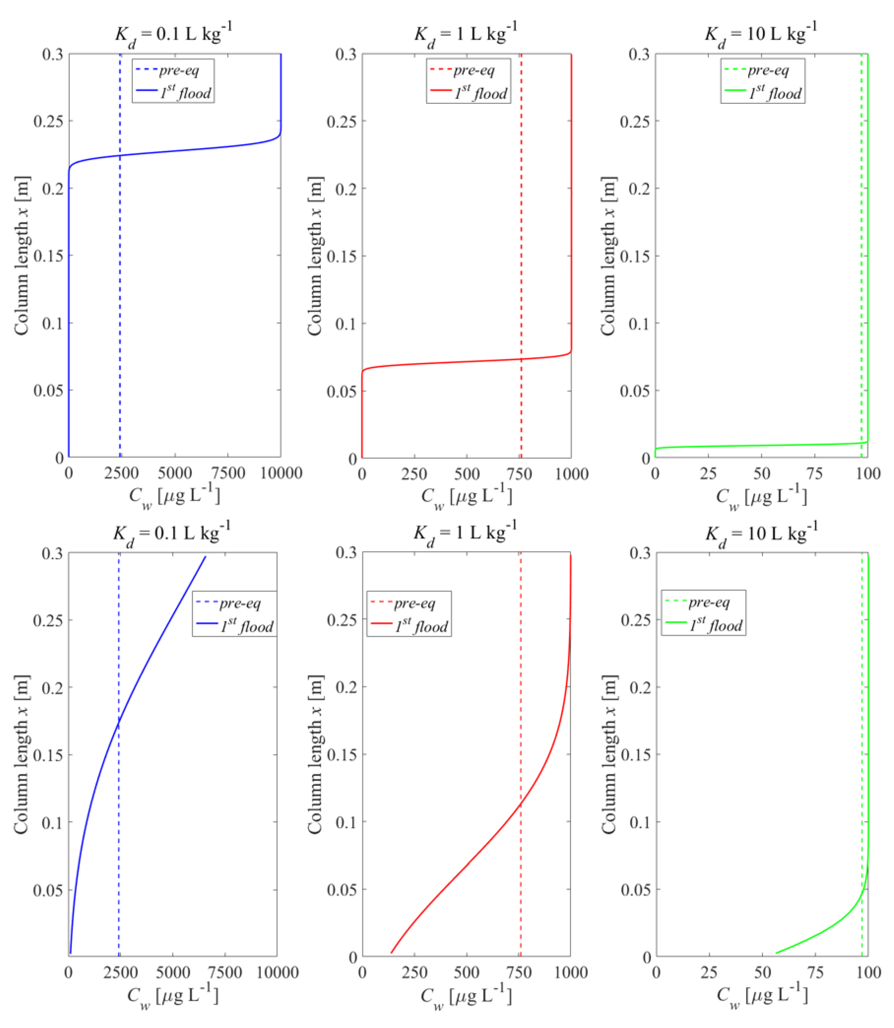
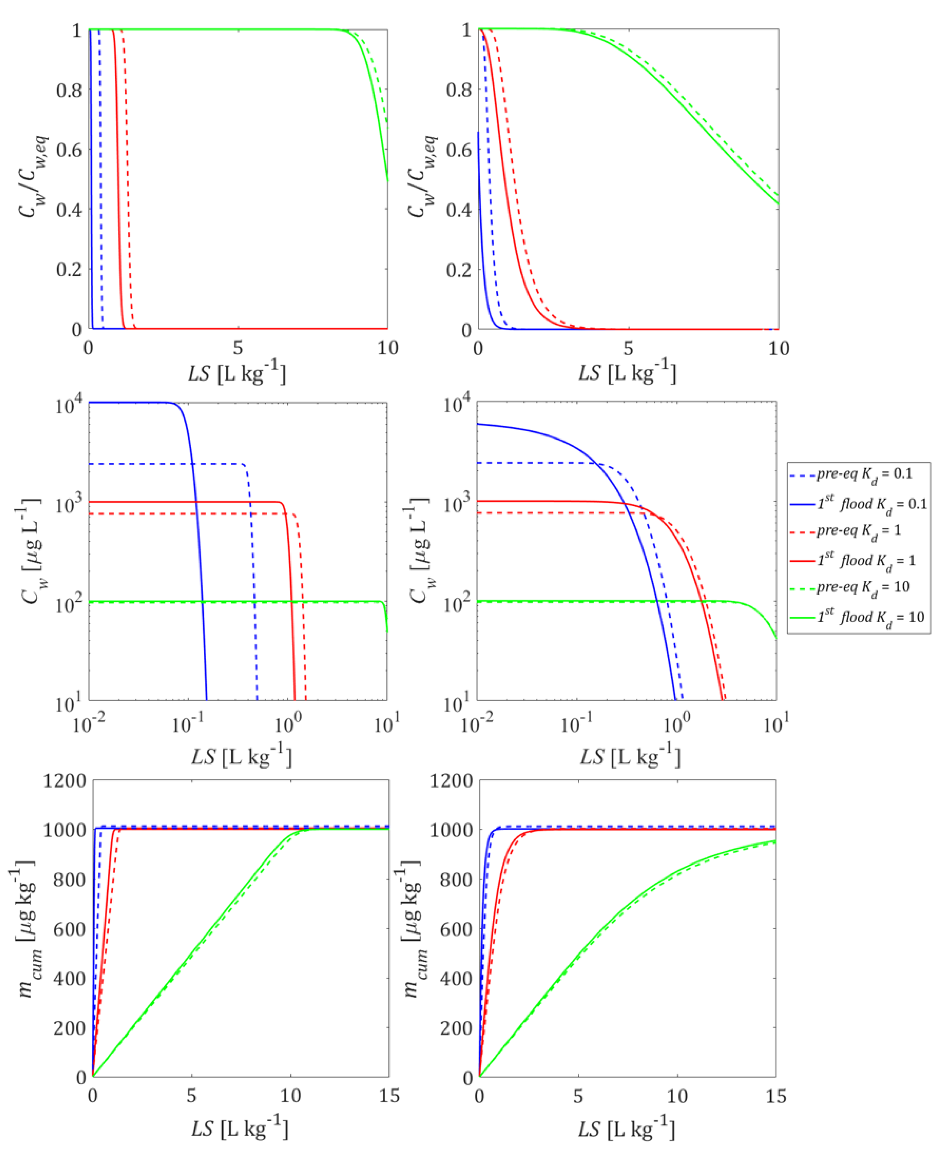
3.1. Impact of Initial Conditions on Leaching

In order to investigate the impact of initial conditions on leaching behavior, we compared two scenarios: (1) a column filled with pre-equilibrated material where the initial concentration distribution in the column was uniform ($C_{w,eq}=C_{s,ini}/\left(K_d+\frac{n}{{\rho }_b}\right)$) and (2) columns with non-uniform concentration distributions after first flooding where concentrations increased towards the outlet (to a maximum of $C_{w,eq}=C_{s,ini}/K_d$) while at the inlet the solute was already depleted. To illustrate this, we used the film diffusion model with fine grain sizes, and thus, fast kinetics (local equilibrium conditions). Figure 4 shows the initial aqueous concentration distribution in the up-flow column test after the first flooding of the column compared to the pre-equilibrium case. The results show that the differences in the initial concentration profiles became smaller with increasing sorption. At high $K_d$ values, the deviation of the initial concentration profiles only occurred at the inlet of the column. At low $K_d$ values, very high concentrations are expected at the column outlet; in extreme cases this may lead to a density increase in the leachate and—especially if flow is stopped—to density driven flow within the column. This would cause dilution and lower leachate concentrations when the flow is restarted as was potentially observed by Naka et al. [36]. Density driven mixing may be caused by soluble materials, e.g., sulphate or other salts and not necessarily the target compounds. This phenomenon is quite similar to the case where the dispersion is taken into account (see bottom curves of Figure 4 and also Figures S1–S8 in SM), which leads to more “mixing” in the column and thus lower initial concentrations at the outlet, especially for low $K_d$ values.

Figure 5 shows how the initial conditions (pre-equilibrated column and column after first flooding) influence the leaching curves. Compared to the pre-equilibrated case, a higher equilibrium concentration appeared at the outlet of the column after the first flooding period and more contaminant mass was released from the column at early times, followed by a rapidly decreasing concentration (see Figure 5, 2nd row). The deviations vanished with increasing $K_d$ and became almost insignificant for $K_d\ge$10 L kg⁻¹. Dispersion also reduces differences between the pre-equilibrated and the first flooding case. At high $K_d$ values, the maximum concentrations were still achieved but the tailings became smoother. With the decrease of the $K_d$ value, the concentration gradients at the inlet became steeper and the “back” dispersion fluxes towards the outlet increased as well. In extreme cases, the peak concentration at the column outlet was smaller than the maximum concentration expected (e.g., $K_d=$ 0.1 L kg⁻¹). The effect of initial conditions on normalized concentrations looks like a phase shift (see Figure 5, 1st row). This would lead to an underestimation of $K_d$ values derived from the pre-equilibrium analytical solution (Equation (4)) if the conditions in the column after the first flooding are not appropriately considered. The lower the $K_d$, the earlier the cumulative leachate concentration reaches its maximum value ($m_{cum,max}=1000\mathsf{\mu }$g kg⁻¹). Dispersion shifts this point to later times (see Figure 5, 3rd row).

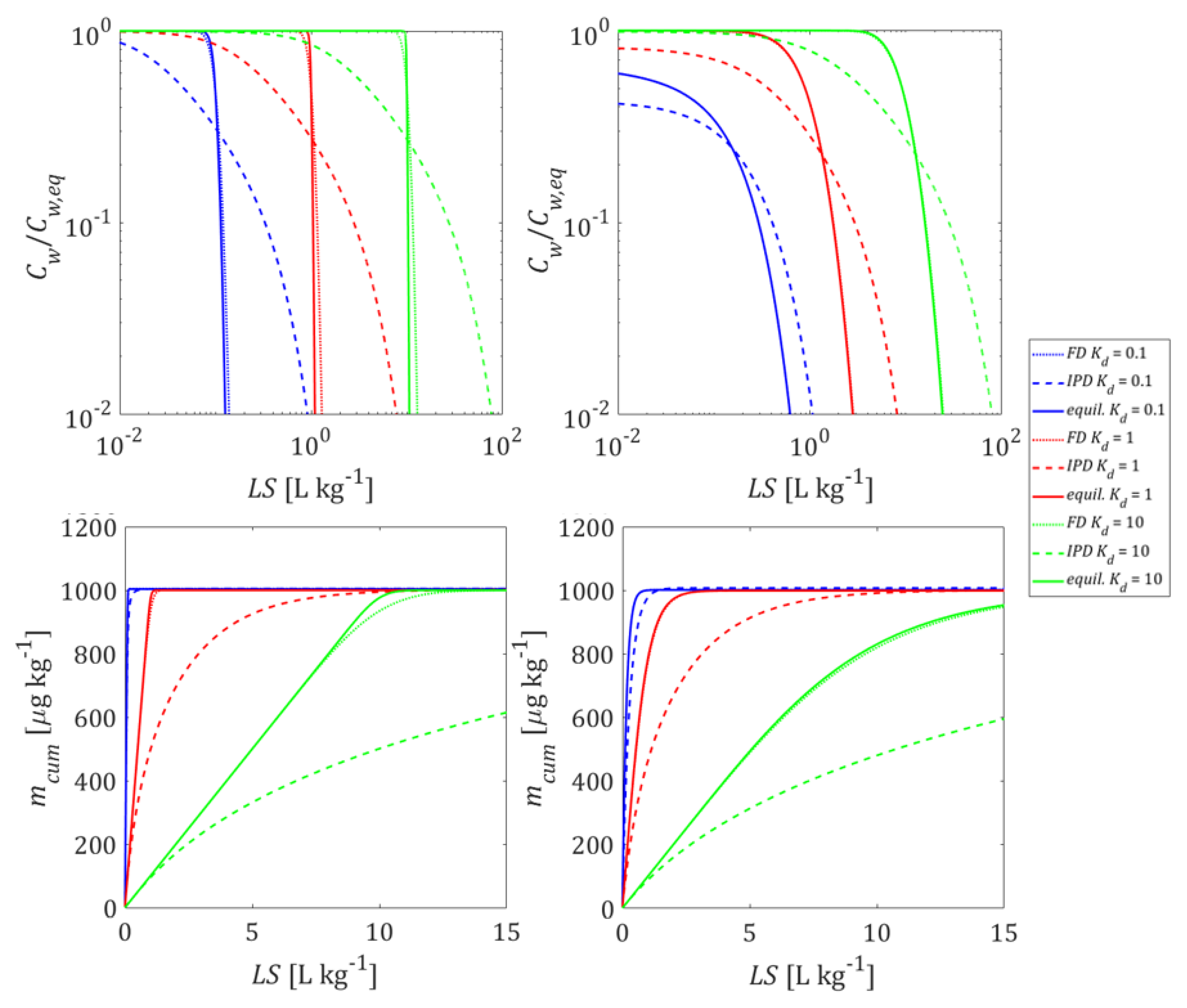
3.2. Initial Conditions and Leaching with Mass Transfer Limitations

Mass-transfer limitations may change the picture considerably, with respect to initial conditions and the development of leachate concentrations over time. Figure 6 shows the influence of film diffusion (FD) compared to intraparticle pore diffusion (IPD) limited desorption on the initial concentration distribution in the column after the first flooding period. For large $K_d$ values, equilibration is achieved after shorter distances in the column because of the retardation of the clean water front. The deviations between FD and IPD are due to different mass transfer zone lengths, $X_{s,63.2\%}$ (see Appendix D for a discussion of the concept and calculation of this length for FD and IPD). For FD, the mass transfer zone length is independent of the $K_d$ value and proportional to the particle size (Equation (A28)). In contrast, for IPD the length of the mass transfer zone increases with particle size to the power of 3/2 ($d^{3/2}$) and decreases with $\sqrt{K_d}$ (Equation (A32)) (e.g., $X_{s,63.2\%}=$ 10 cm, 3.5 cm, and 1.1 cm for $K_d$ values of 0.1 L kg⁻¹, 1 L kg⁻¹ and 10 L kg⁻¹ (see Figure A2)). The length of the mass transfer zone for IPD is much longer than for FD, but differences decrease with increasing $K_d$ values. For $K_d$ values of 1 L kg⁻¹ and 10 L kg⁻¹, the mass transfer zone lengths for IPD are much shorter than the column length ($X_{col}$ = 30 cm), which indicates that the equilibrium concentration is achieved at the outlet of the column after the first flooding. For small $K_d$ values (e.g., $K_d=$ 0.1 L kg⁻¹), the equilibrium concentrations are not achieved at the outlet if dispersion is considered (see Figure 6, lower panel) although the mass transfer zone length ($X_{s,63.2\%}=10\mathrm{cm}$) is still shorter than the column length. This is because the “clean” water front is close to the column outlet and dispersion “dilutes” the steep concentration gradients (“back dispersion”). The deviations between FD and fast kinetics almost vanish when dispersion is considered, indicating that with film diffusion, equilibrium is almost achieved. The development of the concentration distribution for IPD is also illustrated in animated graphs provided in the Supplementary Material (SM).

Figure 7 shows concentrations in aqueous leachates that correspond to the initial conditions shown in Figure 6. If leaching is limited by IPD, then the leaching process is slower and concentrations at early times are considerably lower than in the FD or the equilibrium model. This is due to the retarded diffusive transport within the tortuous intragranular pores and the correspondingly small effective diffusion coefficients ($D_e$). The contaminant release rate becomes lower and lower over time. Leachate concentrations decrease first with the square root of time (typical for transient diffusion) and then exponentially (see Figure 7 without dispersion, and Appendix D for details about the development of the internal mass transfer resistance over time). Note, the cumulative concentration curves confirm the mass conservation of the numerical solutions.

3.3. Nonlinear Sorption Isotherms

For many of the environmental contaminants and solid materials that are typically analyzed in column leaching tests, non-linear sorption isotherms describe the distribution of solutes between the aqueous and solid phases. The significance of this non-linearity for the development of the conditions in the column before the leaching starts has been analyzed exemplarily by defining Freundlich isotherms that result in the same “effective” $K_d$ for the aqueous concentration at equilibrium: $K_{fr}=K_d/C_{w,eq}^{\frac{1}{n}-1}$.

Figure 8 shows the influence of nonlinear sorption on both the initial concentrations in the column and the leaching curves for the example of $K_d$= 1 L kg⁻¹ when no dispersion is considered. The differences in the concentration distribution before percolation starts are moderate. Concentration profiles tend to be smoother with nonlinear sorption with a slightly lower maximum concentration at the column outlet for low to mid $K_d$ values if dispersion is considered (see SM, Figure S1). Differences become more obvious in the tailing part of the leaching curves. Freundlich exponents smaller than 1 result in a longer tailing as is expected. The effect of nonlinear sorption looks similar to the dispersion effect, in both cases the leaching curves show more tailing (see SM, Figure S2). Nonlinearity of sorption is notably less significant than kinetic limitations in the mass transfer mechanisms.

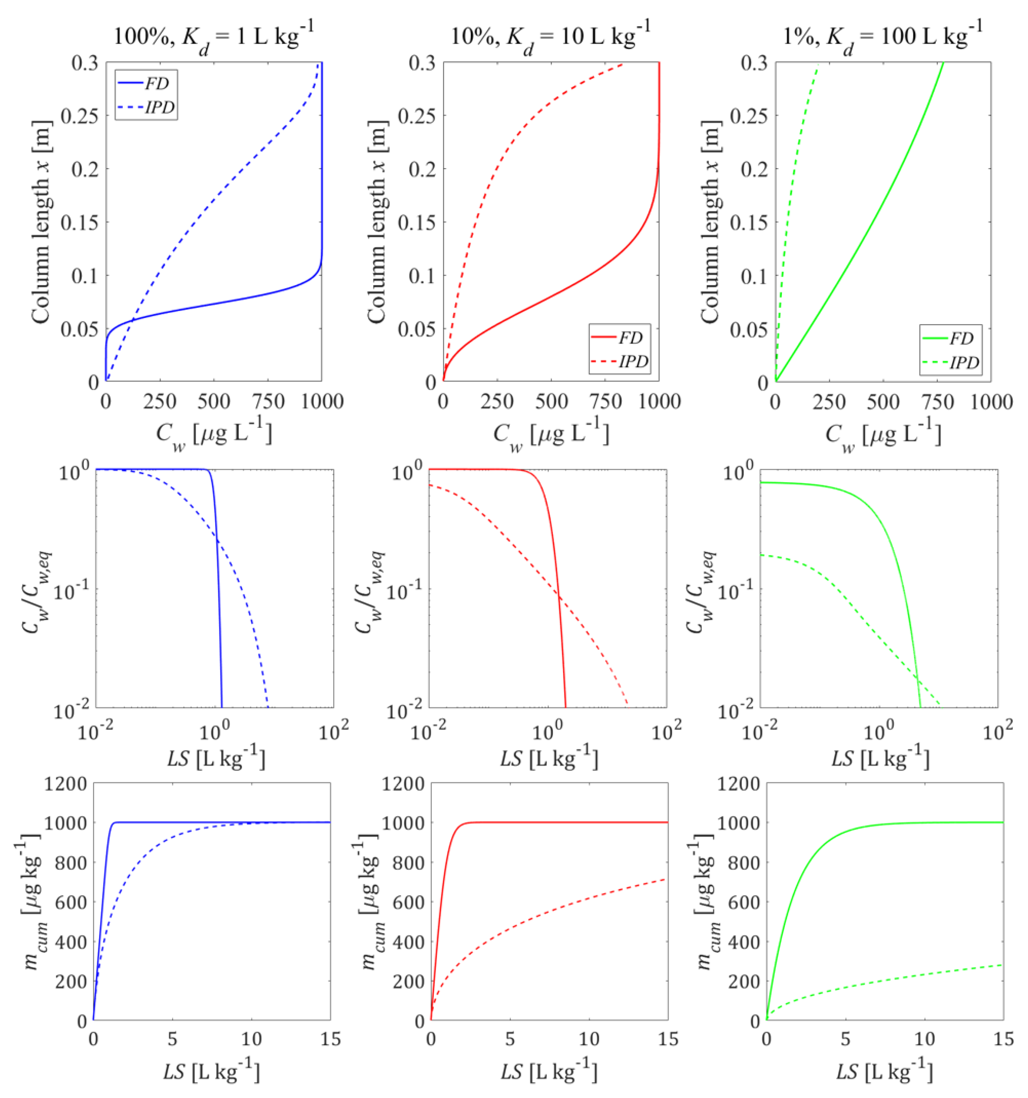
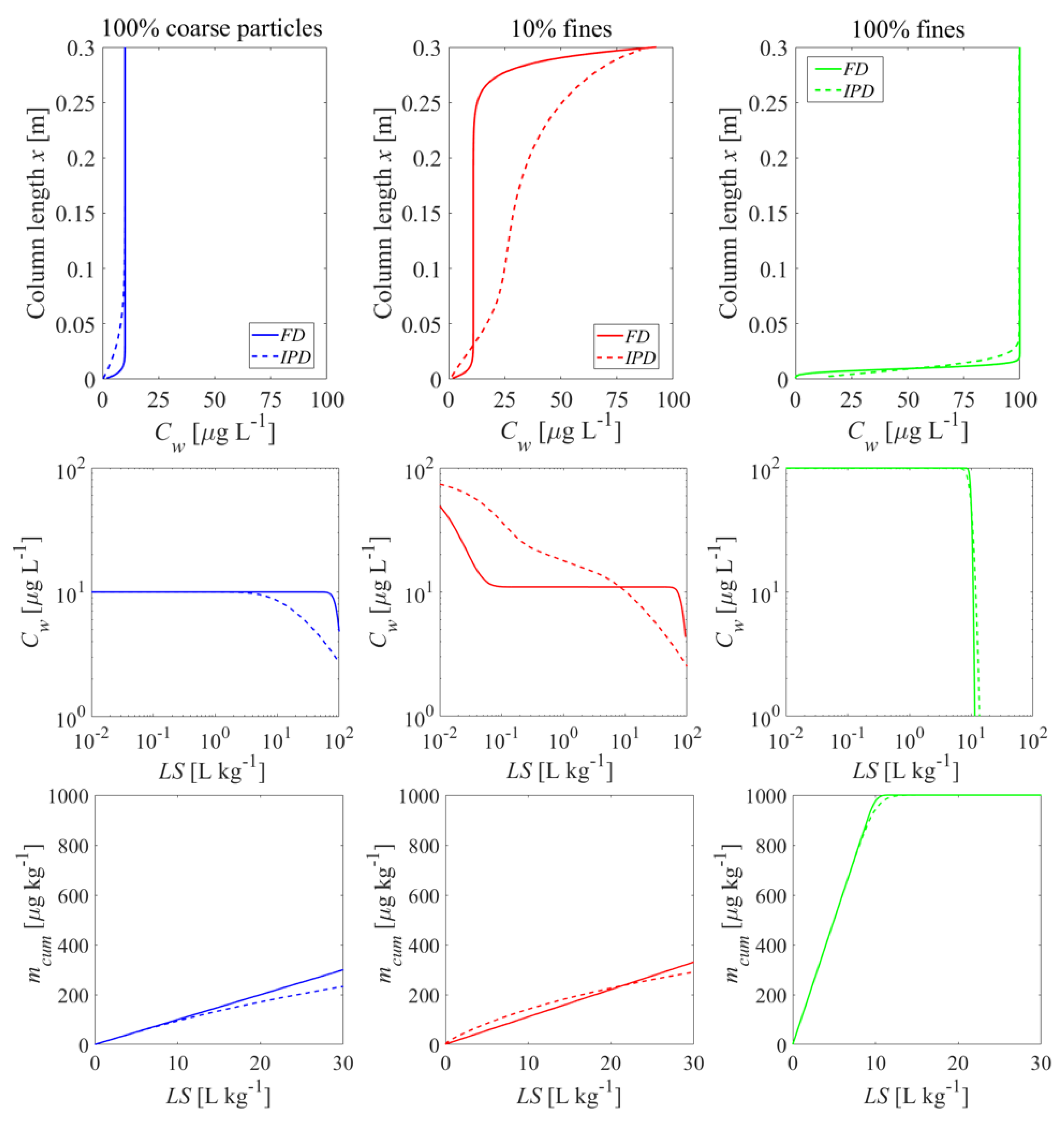
3.4. Impact of Heterogeneous Sample Composition

Real world materials that are typically investigated in leaching tests are not always homogeneous. Although the sample might be addressed as ‘one material’, its individual grains have different sizes and differ most likely also in other properties such as porosity, tortuosity, sorption capacity, etc., and may contain different amounts of the contaminants of interest. In order to illustrate the impact of material heterogeneity, we have carried out several numerical leaching experiments with hypothetical material compositions.

First, we consider three bi-modal material compositions. Each of these compositions consist of a fraction of contaminated particles (e.g., particulate organic carbon particles with high $K_d$) and another fraction of particles that neither contain contaminants nor possess any sorption capacity. If equilibrium conditions prevail during the first flooding and leaching, the heterogeneity of the sample does not matter, it is simply the average $K_d$ ($K_{d,av}$) that rules. The situation changes if mass transfer between the solid and the aqueous phases is limited due to diffusion (FD or IPD). If only a small fraction of the particles in the sample carries the compounds of interest, the volume of particles released by the compound and thus the surface area available for mass transfer becomes much smaller. This may lead to pronounced non-equilibrium conditions after first flooding (see, e.g., Equations (A26) and (A30)) and during leaching. Figure 9 shows a comparison of the initial concentration profiles in the column after the first flooding, as well as the corresponding leaching curves that would develop for the three bi-modal material compositions (100/10/1% of the material is contaminated at a $K_d=1/10/100$ L kg⁻¹, respectively). A small fraction of strong sorbents showed lower desorption rates compared to a large fraction of the weak sorbents. For this “exotic” case where only 1% of the particles carries all the contamination, initial nonequilibrium and long tailing was observed. This effect was very pronounced for intraparticle pore diffusion; the concentrations initially started on a plateau (“like equilibrium”), but then rapidly declined and showed a pronounced tailing and decrease with the square root of time (or LS). It may be noted, that longitudinal dispersion becomes less relevant if non-equilibrium conditions prevail at high $K_d$ values (see Figures S3 and S4 in SM). If such pronounced initial nonequilibrium is observed, then extended periods of time would be needed to equilibrate the water in the column with the solids (e.g., a manifold of the contact time of 5 h).

Samples consisting of mixtures of different particle sizes represent another typical and frequently occurring case of material heterogeneity. To illustrate the impact of such grain size heterogeneity, two bi-modal grain size distributions are considered here, introducing two grain sizes, coarse particles having a diameter of $d_{p,coarse}=$ 2000 $\mathsf{\mu }$m, and fine particles with $d_{p,fine}=$ 63 $\mathsf{\mu }$m. The 1st hypothetical grain size distribution consists of 10% fine particles and 90% coarse particles, the 2nd distribution of 90% fine particles and 10% coarse particles.

If mass transfer is limited by film diffusion, the establishment of the initial conditions as well as leaching (Figure 10) occurs under conditions close to equilibrium for both grain size distributions at all $K_d$ values (0.1, 1, and 10 L kg⁻¹). While the shapes of all leaching curves are very similar, their locations are shifted in time according to the different $K_d$ values by a factor of 10. If intraparticle pore diffusion is considered, tailing is observed if coarse particles predominate. This applies to both, the development of initial conditions in the column and leaching. If fine particles predominate, the leaching is close to equilibrium at early times; at later times, tailing is observed with the typical square root of time behavior. Considering the dispersion effect, non-equilibrium concentrations can be seen at the column effluent after first flooding especially at low $K_d$ values ($K_d=$0.1 L kg⁻¹). Initial non-equilibrium conditions become more salient for intraparticle pore diffusion if coarse particles predominate (see Figures S5 and S6 in SM).

Combining the heterogeneity of particle size ($d$) and sorption capacity ($K_d$), we consider three material compositions in the third case, which aims at showing circumstances where strong non-equilibrium conditions may be expected. For many materials this is probably not very realistic, but it may occur in material mixtures where a small particle fraction carries a “labile” contamination with a low $K_d$ vs. just a few large particles carrying the contaminant with a large $K_d$. A hypothetical mixture containing 10% of fine particles with low sorption capacity ($K_d=$ 10 L kg⁻¹) and 90% of coarse particles with high sorption capacity ($K_d=$ 100 L kg⁻¹) is compared with two extreme cases where a hypothetical sample only contains pure fine particles with low sorption capacity and another hypothetical sample contains pure coarse particles with high sorption capacity. Figure 11 shows the initial concentration distribution for these three compositions after the first flooding period as well as the corresponding leaching curves. Sorption equilibrium is achieved rapidly if the sample consists of only fine particles with a small $K_d$ or only coarse particles with a high $K_d$. Pure coarse material with a high $K_d$ shows a low equilibrium concentration ($C_{w,eq}=C_{s,ini}/K_d=$ 1000 $\mathsf{\mu }$g kg⁻¹$/$100 L kg⁻¹ $=$ 10 $\mathsf{\mu }$g L⁻¹) while pure fine material with a low $K_d$ presents a much higher equilibrium concentration ($C_{w,eq}=C_{s,ini}/K_d=$ 1000 $\mathsf{\mu }$g kg⁻¹/10 L kg⁻¹ = 100 $\mathsf{\mu }$g L⁻¹) after a short flow distance. Interestingly, the mixed case where 10% of the column is fine material caused a high concentration which would be sorbed by the coarse materials leading to a slightly higher plateau concentration compared to pure coarse materials. The pollutants were redistributed between fine and coarse materials during the first flooding of the column. The concentration increase towards the outlet of the column in the mixed case is due to fast desorption from the fine material followed by slow sorption by the coarse material. The redistribution is almost complete at the inlet of the column because of the long residence time ($t_c$= 5 h). Since the fine particles make up only to 10% of the total mass, they are already depleted in contaminant concentrations inside the column and in equilibrium with the coarse particles (reflecting both extreme cases). The front of the high concentration caused by the fine particles is already close to the outlet, while the rest is in equilibrium with the 90% coarse particle fraction.

The leaching curve of the mixed case (red lines) reflects the properties of the two pure (homogeneous) cases with either fine or coarse particles. Ten percent of the fine particles with low sorption capacity led to a peak effluent concentration which was only slightly lower than the equilibrium concentration of the pure fine particles with low sorption capacity. However, because the fine particles made up only 10% of the total mass, this peak concentration leached out rapidly and the eluate concentrations followed the coarse particles with a high sorption capacity for long time periods (blue curves). Although this may appear to indicate non-equilibrium conditions (because of the rapid initial decline of the concentrations followed by a plateau or “tailing”), leaching from fine and coarse particles occurs at, or close to equilibrium. Compared to FD, the IPD in the mixed sample showed a slower concentration decline because of the desorption kinetics of the IPD of the coarse particles was slower than the case of FD and on the long-term control release kinetics. For the cumulative mass release the mixed case is close to the coarse material for both the FD and the IPD, whereas the fine-grained particles showed a much higher and faster release (see Figure 11: bottom panel).

4. Summary and Conclusions

We conducted numerical simulations to investigate the release characteristics of low to strongly sorbing compounds ($K_d=0.1$–$100$ L kg⁻¹) in column leaching tests. Two different scenarios for the establishment of the initial conditions before the start of the leaching phase were considered: a fully pre-equilibrated column and a more realistic scenario where a column is flooded with water from the bottom. In order to highlight the effect of mass transfer limitations, two mechanisms are compared: film diffusion and intra-particle diffusion. Cases without and with dispersion illustrate how dispersive mixing may mask diffusion limited mass transfer. Furthermore, we looked into the impact of heterogeneous sample compositions in terms of reactive particle fractions and particle sizes. Since possible parameter combinations amount to almost infinite numbers, we have limited our analysis to just a few exemplary cases that illustrate the role of individual material properties. These few cases already show that virtually any leaching behavior can be produced with highly heterogeneous samples (depending on the mixing of different materials). The most important conclusions are:

Initial conditions have a significant impact on leaching at low $K_d$ values ($K_d$< 1 L kg⁻¹). With increasing $K_d,$ the differences between pre-equilibrium and non-equilibrium conditions gradually vanish for $K_d$> 10 L kg⁻¹ (see Figure 5). Compounds with very low $K_d$ (“salts”) would reach extremely high concentrations ($K_d$<< 1 L kg⁻¹) at the column outlet (see Figure 4) potentially leading to enhanced dispersion due to density fingering. The $K_d$ values derived from retardation factors ($R_d$ in Equation (4)) would be underestimated if the conditions in the column after the first flooding are not appropriately considered, due to a “phase shift” in normalized concentrations curves ($C_w/C_{w,eq}$ vs. LS).

Dispersion generally causes “smoothing” of concentrations gradients in the column and tends to “mask” film and intraparticle diffusion characteristics due to enhanced “mixing” of the solute within the column. It may lead to smaller initial concentrations at the column outlet after the first flooding period than expected for equilibrium; this is pronounced especially at low $K_d$ values (see Figure 7 and Figure S2), which may be interpreted as non-equilibrium, but is just a consequence of dilution by dispersive mixing.

Intraparticle pore diffusion (IPD) generally shows slower desorption kinetics than film diffusion (FD) through an aqueous boundary layer. This is due to the much smaller effective diffusion coefficient in the intraparticle pores and the large diffusion distance that develops inside the particle over time, resulting in the typical square root of time decrease of concentrations (a slope of 1/2 is observed in log-log plots of leaching curves, see Figure 7, Figure 9 and Figure 10). IPD is more sensitive to the variation of particle sizes than FD (see Figure 10). Mass transfer limitations in an aqueous boundary layer commonly exists for surface adsorbed compounds and easily soluble solids (“salts”). Elements such as heavy metals, which are slowly released from the solid phase, would require much lower solid state diffusion coefficients; if reaction fronts propagate into the particle releasing metals, intraparticle (solid) diffusion models apply again (shrinking core), which are very similar to the IPD approach used here.

Non-linear sorption has little influence on the leaching test results if the “right” effective $K_d$ value is calculated for the proper concentration range (since for the nonlinear sorption the $K_d$ depends on the concentration, large deviations may occur if just the $K_{fr}$ is determined far away of the sample’s concentration is used as “$K_d$”); nevertheless, as concentrations decrease nonlinear sorption causes more tailing (see Figure 8).

Heterogeneous samples with only a small fraction of strongly sorbing particles lead to much slower desorption rates (because of less surface area), especially if mass release is limited by intraparticle pore diffusion (see Figure 9). In extreme cases (just 1% of the material is contaminated at $K_d=100\times K_{d,av}$), leaching may start at a plateau (suggesting equilibrium), but far below equilibrium concentrations ($C_{w,peak}\ll C_{w,eq}$) and concentrations later decrease further; The $K_d$ values derived from the initial aqueous concentration ($K_d=C_{s,ini}/C_{w,peak}$) would be overestimated while the $K_d$ values calculated from retardation factors would be underestimated.

In contrast to that, already relatively small amounts of fine particles lead to initial equilibrium, but long-term tailing occurs and is dominated by the coarse particle fraction, especially for intraparticle pore diffusion. Since our FD simulations are close to equilibrium, results are not very affected by grain size heterogeneity (see Figure 10). Material mixtures of small amounts of fine particles (10%) with low sorption capacity ($K_d=$10 L kg⁻¹) and large amounts of coarse particles with high sorption capacity ($K_d=$ 100 L kg⁻¹), exhibit the respective characteristics of each of the individual components in different time periods (see Figure 11). Small amounts of fine particles with low sorption capacity dominate short term behavior of the mixtures and lead to a peak effluent concentration ($C_{w,peak}$) which approaches the equilibrium concentration expected for fine particles (see Figure 11). Since the mass fraction of fine particles is small (10%), the leachate concentrations drop rapidly and reach slightly higher equilibrium levels of 100% pure coarse particles due to the redistribution of pollutants between fine and coarse particles. Ten percent of fine particles with low sorption capacity causes a high equilibrium concentration which are sorbed by the coarse particles with high sorption capacity. $K_d$ values derived from the initial aqueous concentration ($K_d=C_{s,ini}/C_{w,peak}$) would be underestimated, while $K_d$ values derived from the following plateau concentration would be overestimated. Cumulative mass release, however, is often quite insensitive to mass transfer mechanisms (FD or IPD) especially for LS < 5 (see Figure 11).

References

1. Röhler, K.; Haluska, A.A.; Susset, B.; Liu, B.; Grathwohl, P. Long-term behavior of PFAS in contaminated agricultural soils in Germany. J. Contam. Hydrol. 2021, 241, 103812. [Google Scholar] [CrossRef] [PubMed]
2. Löv, Å.; Larsbo, M.; Sjöstedt, C.; Cornelis, G.; Gustafsson, J.P.; Kleja, D.B. Evaluating the ability of standardised leaching tests to predict metal(loid) leaching from intact soil columns using size-based elemental fractionation. Chemosphere 2019, 222, 453–460. [Google Scholar] [CrossRef] [PubMed]
3. Inui, T.; Hori, M.; Takai, A.; Katsumi, T. Column percolation tests for evaluating the leaching behavior of marine sediment containing non-anthropogenic arsenic. In Proceedings of the 8th International Congress on Environmental Geotechnics (from 28th October to 1st November 2018 in Hangzhou, China); Zhan, L., Chen, Y., Bouazza, A., Eds.; Springer: Singapore, 2019; Volume 1. ICEG 2018, Environmental Science and Engineering. [Google Scholar] [CrossRef]
4. Kalbe, U.; Bandow, N.; Bredow, A.; Mathies, H.; Piechotta, C. Column leaching tests on soils containing less investigated organic pollutants. J. Geochem. Explor. 2014, 147, 291–297. [Google Scholar] [CrossRef]
5. Zhu, Y.; Hu, Y.; Guo, Q.; Zhao, L.; Li, L.; Wang, Y.; Hu, G.; Wibowo, H.; Francesco, D.M. The effect of wet treatment on the distribution and leaching of heavy metals and salts of bottom ash from municipal solid waste incineration. Environ. Eng. Sci. 2021. ahead of print. [Google Scholar] [CrossRef]
6. Kumar, A.; Samadder, S.R.; Kumar, V. Assessment of groundwater contamination risk due to fly ash leaching using column study. Environ. Earth Sci. 2019, 78, 18. [Google Scholar] [CrossRef]
7. Chan, W.P.; Ren, F.; Dou, X.; Yin, K.; Chang, V.W.C. A large-scale field trial experiment to derive effective release of heavy metals from incineration bottom ashes during construction in land reclamation. Sci. Total Environ. 2018, 637, 182–190. [Google Scholar] [CrossRef] [PubMed]
8. Di Gianfilippo, M.; Costa, G.; Verginelli, I.; Gavasci, R.; Lombardi, F. Analysis and interpretation of the leaching behaviour of waste thermal treatment bottom ash by batch and column tests. Waste Manag. 2016, 56, 216–228. [Google Scholar] [CrossRef]
9. Tsiridis, V.; Petala, M.; Samaras, P.; Sakellaropoulos, G.P. Evaluation of interactions between soil and coal fly ash leachates using column percolation tests. Waste Manag. 2015, 43, 255–263. [Google Scholar] [CrossRef]
10. Lange, C.N.; Flues, M.; Hiromoto, G.; Boscov, M.E.G.; Camargo, I.M.C. Long-term leaching of As, Cd, Mo, Pb, and Zn from coal fly ash in column test. Environ. Monit. Assess. 2019, 191, 602. [Google Scholar] [CrossRef]
11. Liu, B.; Li, J.; Wang, Z.; Zeng, Y.; Ren, Q. Long-term leaching characterization and geochemical modeling of chromium released from AOD slag. Environ. Sci. Pollut. Res. 2020, 27, 921–929. [Google Scholar] [CrossRef]
12. Schwab, O.; Bayer, P.; Juraske, R.; Verones, F.; Hellweg, S. Beyond the material grave: Life Cycle Impact Assessment of leaching from secondary materials in road and earth constructions. Waste Manag. 2014, 34, 1884–1896. [Google Scholar] [CrossRef]
13. Diotti, A.; Galvin, A.P.; Piccinali, A.; Plizzari, G.; Sorlini, S. Chemical and leaching behavior of construction and demolition wastes and recycled aggregates. Sustainability 2020, 12, 10326. [Google Scholar] [CrossRef]
14. Liu, H.; Zhang, J.; Li, B.; Zhou, N.; Xiao, X.; Li, M.; Zhu, C. Environmental behavior of construction and demolition waste as recycled aggregates for backfilling in mines: Leaching toxicity and surface subsidence studies. J. Hazard. Mater. 2020, 389, 121870. [Google Scholar] [CrossRef] [PubMed]
15. Bandow, N.; Finkel, M.; Grathwohl, P.; Kalbe, U. Influence of flow rate and particle size on local equilibrium in column percolation tests using crushed masonry. J. Mater. Cycles Waste Manag. 2019, 21, 642–651. [Google Scholar] [CrossRef]
16. Butera, S.; Hyks, J.; Christensen, T.H.; Astrup, T.F. Construction and demolition waste: Comparison of standard up-flow column and down-flow lysimeter leaching tests. Waste Manag. 2015, 43, 386–397. [Google Scholar] [CrossRef]
17. Chen, Z.; Zhang, P.; Brown, K.; Branch, J.; van der Sloot, H.; Meeussen, J.; Delapp, R.; Um, W.; Kosson, D. Development of a geochemical speciation model for use in evaluating leaching from a cementitious radioactive waste form. Environ. Sci. Technol. 2021, 55, 8642–8653. [Google Scholar] [CrossRef]
18. Molleda, A.; López, A.; Cuartas, M.; Lobo, A. Release of pollutants in MBT landfills: Laboratory versus field. Chemosphere 2020, 249, 126145. [Google Scholar] [CrossRef]
19. Grathwohl, P.; van der Sloot, H. Groundwater risk assessment at contaminated sites (GRACOS): Test methods and modelling approaches. In Groundwater Science and Policy; Quevauviller, P., Ed.; RSC Publishing: Cambridge, UK, 2007. [Google Scholar]
20. Susset, B.; Grathwohl, P. Leaching standards for mineral recycling materials—A harmonized regulatory concept for the upcoming German Recycling Decree. Waste Manag. 2011, 31, 201–214. [Google Scholar] [CrossRef] [PubMed]
21. Grathwohl, P.; Susset, B. Comparison of percolation to batch and sequential leaching tests: Theory and data. Waste Manag. 2009, 29, 2681–2688. [Google Scholar] [CrossRef] [PubMed]
22. Grathwohl, P. On equilibration of pore water in column leaching tests. Waste Manag. 2014, 34, 908–918. [Google Scholar] [CrossRef]
23. Grathwohl, P.; Reinhard, M. Desorption of Trichloroethylene in Aquifer Material: Rate Limitation at the Grain Scale. Environ. Sci. Technol. 1993, 27, 2360–2366. [Google Scholar] [CrossRef]
24. Rügner, H.; Kleineidam, S.; Grathwohl, P. Long term sorption kinetics of phenanthrene in aquifer materials. Environ. Sci. Technol. 1999, 33, 1645–1651. [Google Scholar] [CrossRef]
25. Wang, G.; Kleineidam, S.; Grathwohl, P. Sorption/desorption reversibility of phenanthrene in soils and carbonaceous materials. Environ. Sci. Technol. 2007, 41, 1186–1193. [Google Scholar] [CrossRef]
26. Finkel, M.; Grathwohl, P. Impact of pre-equilibration and diffusion limited release kinetics on effluent concentration in column leaching tests: Insights from numerical simulations. Waste Manag. 2017, 63, 58–73. [Google Scholar] [CrossRef] [PubMed]
27. Kleineidam, S.; Rügner, H.; Grathwohl, P. Impact of grain scale heterogeneity on slow sorption kinetics. Environ. Toxicol. Chem. 1999, 18, 1673–1678. [Google Scholar] [CrossRef]
28. Jäger, R.; Liedl, R. Prognose der Sorptionskinetik organischer Schadstoffe in heterogenem Aquifermaterial (Predicting sorption kinetics of organic contaminants in heterogeneous aquifer material). Grundwasser 2000, 5, 57–66. [Google Scholar] [CrossRef]
29. Xiao, Y.; Feng, Z.; Huang, X.; Huang, L.; Chen, Y.; Wang, L.; Long, Z. Recovery of rare earths from weathered crust elution-deposited rare earth ore without ammonia-nitrogen pollution: I. leaching with magnesium sulfate. Hydrometallurgy 2015, 153, 58–65. [Google Scholar] [CrossRef]
30. Yin, K.; Chan, W.P.; Dou, X.; Lisak, G.; Chang, V.W.C. Kinetics and modeling of trace metal leaching from bottom ashes dominated by diffusion or advection. Sci. Total Environ. 2020, 719, 137203. [Google Scholar] [CrossRef] [PubMed]
31. Ogata, A.; Banks, R.B. A solution of the differential equation of longitudinal dispersion in porous media. In Professional Paper; Geological Survey (U.S.): Washington, DC, USA, 1961; pp. A1–A7. [Google Scholar]
32. Boving, T.; Grathwohl, P. Matrix diffusion coefficients in sandstones and limestones: Relationship to permeability and porosity. J. Contam. Hydrol. 2001, 53, 85–100. [Google Scholar] [CrossRef]
33. Kalbe, U.; Berger, W.; Eckardt, J.; Simon, F.G. Evaluation of leaching and extraction procedures for soil and waste. Waste Manag. 2008, 28, 1027–1038. [Google Scholar] [CrossRef]
34. Kalbe, U.; Berger, W.; Simon, F.G.; Eckardt, J.; Christoph, G. Results of interlaboratory comparisons of column percolation tests. J. Hazard. Mater. 2007, 148, 714–720. [Google Scholar] [CrossRef]
35. Liu, Y.; Illangasekare, T.H.; Kitanidis, P.K. Long-term mass transfer and mixing-controlled reactions of a DNAPL plume from persistent residuals. J. Contam. Hydrol. 2014, 157, 11–24. [Google Scholar] [CrossRef]
36. Naka, A.; Yasutaka, T.; Sakanakura, H.; Kalbe, U.; Watanabe, Y.; Inoba, S.; Takeo, M.; Inui, T.; Katsumi, T.; Fujikawa, T.; et al. Column percolation test for contaminated soils- Key factors for standardization. J. Hazard. Mater. 2016, 320, 326–340. [Google Scholar] [CrossRef] [Green Version]
37. Arters, D.C.; Fan, L.S. Experimental methods and correlation of solid-liquid mass transfer in fluidized beds. Chem. Eng. Sci. 1990, 45, 965–975. [Google Scholar] [CrossRef]
38. Blasius, H. Grenzschichten in Flüssigkeiten mit kleiner Reibung (The boundary layers in fluids with little friction). J. Appl. Math. Phys. 1908, 56, 1–37. [Google Scholar]
39. Calderbank, P.H.; Moo-Young, M.B. The continuous phase heat and mass transfer properties of dispersions. Chem. Eng. Sci. 1995, 50, 3921–3934. [Google Scholar] [CrossRef]
40. Kirwan, J.; Armenante, P.M. Mass transfer to microparticle systems. Chem. Eng. Sci. 1989, 44, 2781–2796. [Google Scholar] [CrossRef]
41. Levins, D.M.; Glastonbury, J.R. Application of Kolmogorofff’s theory to particle-liquid mass transfer in agitated vessels. Chem. Eng. Sci. 1972, 27, 537–543. [Google Scholar] [CrossRef]
42. Mao, H.; Chisti, Y.; Moo-Young, M. Multiphase hydrodynamics and solid-liquid mass transfer in an external-loop airlift reactor- a comparative study. Chem. Eng. Commun. 1992, 113, 1–13. [Google Scholar] [CrossRef]
43. Ohashi, H.; Sugawara, T.; Kikuchi, K.I. Mass transfer between particles and liquid in solid-liquid two-phase flow through vertical tubes. J. Chem. Eng. Jpn. 1981, 14, 489–491. [Google Scholar] [CrossRef] [Green Version]
44. Sherwood, T.K.; Pigford, R.L.; Wilke, R.L. “Mass Transfer”; McGraw-Hill: New York, NY, USA, 1975. [Google Scholar]
45. Cirpka, O.A. Solute and heat transport. In Lecture Notes “Environmental Modeling 2”; 2020; (unpublished, University of Tübingen). [Google Scholar]
46. Liedl, R.; Ptak, T. Modelling of diffusion-limited retardation of contaminants in hydraulically and lithologically nonuniform media. J. Contam. Hydrol. 2003, 66, 239–259. [Google Scholar] [CrossRef]
Figure 1. Initial concentration distribution in a column of length x for the “pre-equilibrated” case (dashed line) and after the first flooding of an initially dry column from the bottom (solid line); no dispersion, R d = 2 , after Grathwohl and Susset, 2009 [21].
Materials 14 04708 g001
Figure 2. Scheme of mass transfer limited by film diffusion during the first flooding with fixed concentration at the interface (because the infiltrating water is always contacting fresh material as it advances).
Materials 14 04708 g002
Figure 3. Scheme of mass transfer limited by intraparticle pore diffusion.
Materials 14 04708 g003
Figure 4. Initial aqueous concentration distributions in the column after the first flooding (solid lines) if mass transfer is controlled by film diffusion for three different distribution coefficients, K d , compared to the pre-equilibrated case (dashed lines). Top panel: without dispersion; bottom panel: with dispersion; n = 0.45, v = 1.67 × 10⁻⁵ m s−1, α /x = 0 or 0.1, C s , i n i = 1000 μ g kg−1, t c = 5 h, d p , f i n e = 63   μ m.
Materials 14 04708 g004
Figure 5. Normalized and absolute concentration ( C w / C w , e q , C w ) as well as cumulative concentration ( m c u m ) in the column effluent vs. time (expressed as liquid to solid ratio: LS) for the initial conditions (depicted in Figure 4) established after the first flooding of the column (solid lines) compared to the pre-equilibrated case (dashed lines). Left column: without dispersion; right column: with dispersion.
Materials 14 04708 g005
Figure 6. Initial aqueous concentration distributions in the column after the first flooding depending on the mass transfer limitation; dotted lines: film diffusion (FD), dashed lines: intraparticle diffusion (IPD); solid lines: fast kinetics (equilibrium, fine particles). Top panel: without dispersion; bottom panel: with dispersion; n = 0.45, v = 1.67 × 10⁵ m s1, α /x = 0 or 0.1, C s , i n i = 1000 μ g kg1, t c = 5 h, D a q = 1 × 10⁹ m2 s1, ε = 0.05, d p , c o a r s e = 2000 μ m, d p , f i n e = 63 μ m.
Materials 14 04708 g006
Figure 7. Normalized concentrations ( C w / C w , e q ) as well as cumulative concentrations ( m c u m ) in the column effluent vs. time (expressed as liquid to solid ratio: LS) for different mass-transfer processes, given the initial conditions depicted in Figure 6. Left column: without dispersion; Right column: with dispersion.
Materials 14 04708 g007
Figure 8. Influence of sorption non-linearity: initial aqueous concentration distribution in the column after the first flooding (left graph) and column effluent concentration (normalized: mid graph, cumulative: right graph) vs. time (expressed as liquid to solid ratio: LS); solid lines: linear sorption ( K d = 1 L kg−1); dashed lines: non-linear sorption case (Freundlich coefficient K f r = 7.94, exponent 1 / n = 0.7); n = 0.45, v = 1.67 × 10⁻⁵ m s−1, α /x = 0 or 0.1, C s , i n i = 1000 μ g kg−1, t c = 5 h, D a q = 1 × 10⁻⁹ m2 s−1, ε = 0.05, d p , c o a r s e = 2000 μ m.
Materials 14 04708 g008
Figure 9. Behavior of bi-modal material compositions of sorbing and non-sorbing particles: initial concentration distribution in the column after the first flooding (top panel) and column effluent concentration (normalized: mid panel, cumulative: bottom panel) vs. time (expressed as liquid to solid ratio: LS). Left column: homogeneous case with average K d   (= K d , a v   = 1 L kg−1); mid column: only 10% of the particles carry the contaminant at K d   =   10 × K d , a v ; right column: only 1% of the particles carry the contaminant at K d = 100 × K d , a v ; the average K d , a v of the entire material is the same for all compositions; solid lines: film diffusion cases, dashed lines: intraparticle diffusion case; n = 0.45, v = 1.67 × 10⁻⁵ m s−1, α = 0 (no dispersion), C s , i n i = 1000 μ g kg−1, t c = 5 h, D a q = 1 × 10⁻⁹ m2 s−1, ε = 0.05,   d p , c o a r s e = 2000 μ m.
Materials 14 04708 g009
Figure 10. Behavior of the bi-modal material compositions of fine and coarse particles: initial concentration distribution in the column after the first flooding (top panel) and column effluent concentration (normalized: mid panel, cumulative: bottom panel) vs. time (expressed as liquid to solid ratio: LS); solid lines: fine particle mass fraction 10%; dashed lines: fine particle mass fraction 90%. (n = 0.45, v = 1.67 × 10⁻⁵ m s−1, α = 0 (no dispersion), C s , i n i = 1000 μ g kg−1, t c = 5 h, D a q = 1 × 10⁻⁹ m2 s−1, ε = 0.05,   d p , c o a r s e = 2000 μ m, d p , f i n e = 63 μ m).
Materials 14 04708 g010
Figure 11. Behavior of bi-modal material compositions of fine particles with low sorption capacity ( K d = 10 L kg1) and coarse particles with high sorption capacity ( K d = 100 L kg1): initial concentration distributions in the column after the first flooding (top panel) and the column effluent concentration (normalized: mid panel, cumulative: bottom panel) vs. time (expressed as liquid to solid ratio: LS). Left column: 100% coarse particles; mid column: mixed sample with 10% fine particles; right column: 100% fine particles; n = 0.45, v = 1.67 × 10⁻⁵ m s−1, α = 0 (no dispersion), C s , i n i = 1000 μ g kg−1, t c = 5 h, D a q = 1 × 10⁻⁹ m2 s−1, ε = 0.05,   d p , c o a r s e   = 2000   μ m, d p , f i n e = 63   μ m.
Materials 14 04708 g011