Consistent Thermo-Capillarity and Thermal Boundary Conditions for Single-Phase Smoothed Particle Hydrodynamics

Abstract

A model for capillary phenomena including temperature-dependency and thermal boundary conditions is presented in the numerical framework of smoothed particle hydrodynamics (SPH). The model requires only a single fluid phase and is therefore computationally more efficient than surface tension schemes which need an explicit fluid-fluid or fluid-gas interface. The model makes use of a surface identification mechanism based on the SPH renormalization tensor. All relevant properties of the continuum surface force (CSF) based approach, i.e., the delta function, normal vector and curvature, are calculated in a consistent manner. The model is parametrized by physical material properties and is successfully validated by means of a large set of analytical test cases. The applicability of the proposed model to more complex scenarios is demonstrated.

1. Introduction

Modeling surface tension in the framework of smoothed particle hydrodynamics [1,2] is generally done using one of the following two approaches.

On the one hand, surface tension can be formulated as a continuum surface force. This approach introduces a surface delta function to approximate the tension, i.e., a force per area, in form of a force per volume [3]. A color function is used here to identify the involved phase and the interface between them. An early SPH implementation of the CSF approach for two phases was described and analyzed by Morris [4]. Hu and Adams [5] used an interface stress tensor to avoid the explicit calculation of the curvature at the phase interface. They also extended the formulation to more than two phase which allows modeling of contact angles. Adami et al. [6] improved the CSF scheme by an accurate curvature calculation. Their method is also able to handle large density ratios of the involved phases of up to 1000. Zhang [7] enabled surface tension modeling in a single-phase SPH simulation by identifying the boundary particles and reconstructing the phase surface in two dimensions (2D) or three dimensions (3D). Breinlinger et al. [8] were able to model wetting effects in two-phase SPH simulations by prescribing the contact angle with respect to a rigid substrate. Thermo-capillary effects based on a temperature-dependent surface tension were studied by Tong and Browne [9] using a two-phase SPH approach. For this purpose, they used a projection of the gradient operator onto the phase interface. Yeganehdoust et al. [10] developed a method to extrapolate the color function into a substrate in order to model both static and dynamic wetting phenomena. Huber et al. [11] introduced a balance equation for the contact line between the two fluid phases and the substrate to accurately model advancing and receding contact angles in dynamic wetting situations. Ordoubadi et al. [12] used a single-phase SPH formulation for the CSF approach in which they identified the surface by a combination of a geometric interface tracking and the calculation of the position divergence field [13]. Hirschler et al. [14] formulated a single-phase model which obtains the surface normal and the surface delta function directly from the SPH kernel gradient. The surface curvature is obtained using a corrected kernel gradient [15]. Krimi et al. [16] used an interface stress tensor formulation to model multi-phase flow situations with large density ratios of the involved phases. Hopp-Hirschler et al. [17] investigated thermo-capillary phenomena in internal flow situations or for two-phase systems, respectively. They stabilized the SPH simulations by a particle shifting technique [18]. Lin et al. [19] proposed the detection of an interface between two phases as well as the calculations of the interface normal and curvature based on a Delaunay triangulation. Fürstenau et al. [20] formulated a single-phase description using the position divergence to identify the surface and SPH kernel gradient to compute the surface normal. They improved the surface curvature calculation by using a curvature tensor. Liu et al. [21] proposed a machine learning approach in order to obtain a more accurate local interface curvature in two-phase simulations. Härdi et al. [22] investigated wetting phenomena of thin films by using an SPH discretization of the shallow water equation and introducing a contact line force. Liu et al. [23] proposed a single-phase surface tension model based on the ${\delta }^{+}$ SPH scheme [24]. They calculated the surface normal from the kernel gradient and used a normalization procedure to improve the accuracy of the surface delta function.

On the other hand, a surface tension formulation can be based on an additional pairwise force which is repulsive at short range, attractive at intermediate range and vanishing at long range. Such models were developed by Nugent and Posch [25] and refined by Tartakovsky and Meakin [26] as well as Akinci et al. [27]. A pairwise force mimics the molecular origin of surface tension [28] and results in a net force towards the bulk for particles at a curved, convex surface [29]. The pairwise force approach originally required calibration by adjusting model parameters which have no correspondence in experiments. Tartakovsky and Panchenko [30] made inroads to overcome this drawback by deriving relations between the pairwise model parameters and physical properties for multi-phase systems. Nair and Pöschel [31] extended this approach to single-phase simulations. Bao et al. [32] improved the pairwise force formulation for dynamic wetting phenomena by introducing an apparent viscosity at the interface to a rigid substrate which mimics the effect of a finite slip length.

In this work a CSF single-phase surface tension scheme is presented which is an extension of an earlier work by the author [33]. The approach for modeling wetting behavior is adapted from Breinlinger et al. [8] and the method to incorporate thermo-capillarity from Tong and Browne [9]. The novelty of the present work is the consistent formulation which is used to compute all surface related properties. The surface identification scheme from Marrone et al. [34], relying on the renormalization tensor, is used as the basis to obtain the surface normal, surface curvature and surface delta function in a consistent and accurate manner. In previous works, at least one of these three surface properties was not based on the renormalization tensor, leading to an inconsistency in the definition of the actual surface. The surface delta function is also used to formulate thermal boundary conditions which take into account heat transfer, heat flux and radiation.

The remaining part of this paper is organized as follows. Section 2 outlines the governing equations and presents all relevant ingredients of the numerical model. Section 3 uses several benchmark cases to assess the predictive quality of the model. The obtained results are discussed in Section 4. Section 5 concludes the main part of the paper. Details of the surface delta function computation are given in Appendix A.

2. Materials and Methods

The governing equations with respect to mass balance, momentum balance and energy balance are presented in Section 2.1 with focus on the surface related terms. The discretization of the governing equations using SPH is described in detail in Section 2.2. The main contribution of the present work is the SPH surface treatment presented in Section 2.2.2. It forms the basis for modeling surface thermal boundary conditions (Section 2.2.4), surface tension (Section 2.2.10) and surface wetting (Section 2.2.11).

2.1. Governing Equations

The evolution of density $\rho$ over time t is given by the mass balance equation,

$$\frac{\mathrm{D}\rho }{\mathrm{D}t}=-\rho \nabla ·\mathbf{v},$$

(1)

where $\mathbf{v}$ is the velocity.

The Navier–Stokes momentum equation provides the time evolution of velocity,

$$\begin{array}{cc}\hfill \frac{\mathrm{D}\mathbf{v}}{\mathrm{D}t}& =-\frac{1}{\rho }\nabla P+\frac{2\eta }{\rho }\nabla ·\mathbb{E}+\frac{1}{\rho }{\mathbf{F}}^{\mathrm{S}}+\mathbf{g}\hfill \\ \hfill & =-\frac{1}{\rho }\nabla P+\frac{\eta }{\rho }{\nabla }^2\mathbf{v}+\frac{1}{\rho }{\mathbf{F}}^{\mathrm{S}}+\mathbf{g},\hfill \end{array}$$

(2)

with pressure P, dynamic viscosity $\eta$, rate of strain tensor $\mathbb{E}=(\nabla \mathbf{v}+{(\nabla \mathbf{v})}^{\mathrm{T}})/2$, volumetric surface tension force ${\mathbf{F}}^{\mathrm{S}}$ and gravitational acceleration $\mathbf{g}$. The time evolution of the position $\mathbf{r}$ is simply

$$\frac{\mathrm{D}\mathbf{r}}{\mathrm{D}t}=\mathbf{v}.$$

(3)

The surface tension force can be decomposed into components normal and tangential, respectively, to the surface,

$${\mathbf{F}}^{\mathrm{S}}={\mathbf{F}}^{\mathrm{n}}+{\mathbf{F}}^{\mathrm{t}}.$$

(4)

The CSF model converts a force per area, i.e., pressure or tension, into a force per volume by multiplication with a delta function ${\delta }_{\mathrm{S}}$ which marks the location of the surface in space. This approach yields the following expression for the normal component of the volumetric surface tension force,

$${\mathbf{F}}^{\mathrm{n}}=-{\sigma }_{\mathrm{n}}\kappa {\delta }_{\mathrm{S}}\mathbf{n}$$

(5)

with ${\sigma }_{\mathrm{n}}$ as the surface tension, $\kappa$ as the curvature and $\mathbf{n}$ as the surface unit normal vector. A corresponding tangential volumetric force caused by a gradient of the surface tension is given by

$${\mathbf{F}}^{\mathrm{t}}={\delta }_{\mathrm{S}}{\nabla }_{\mathrm{S}}{\sigma }_{\mathrm{n}}$$

(6)

with ${\nabla }_{\mathrm{S}}$ as the Nabla operator along the surface. One reason for a non-constant surface tension is a dependency on temperature T which might be expressed as ${\nabla }_{\mathrm{S}}{\sigma }_{\mathrm{n}}={\sigma }_{\mathrm{t}}{\nabla }_{\mathrm{S}}T$ with ${\sigma }_{\mathrm{t}}=\partial {\sigma }_{\mathrm{n}}/\partial T$ which is typically negative and causes Marangoni flow along the surface from warm towards cold regions. The delta function is constructed as the magnitude of the gradient of a color function which is 1 on one side of the surface (or interface) and 0 on the other side.

The evolution for the thermal energy per unit mass H is given by

$$\frac{\mathrm{D}H}{\mathrm{D}t}=\frac{k}{\rho }{\nabla }^{2}T+\frac{q}{\rho }{\delta }_{\mathrm{S}}-\frac{f}{\rho }{\delta }_{\mathrm{S}}(T-T_{\mathrm{a}})-\frac{\epsilon }{\rho }{\sigma }_{\mathrm{B}}{\delta }_{\mathrm{S}}(T^4-T_{\mathrm{a}}^4).$$

(7)

Here, k is the thermal conductivity, q is the heat flux, f is the heat transfer coefficient, $ϵ$ is the emissivity, ${\sigma }_{\mathrm{B}}$ is the Stefan–Boltzmann constant and $T_{\mathrm{a}}$ is the ambient temperature.

The heat capacity c relates the temperature to the specific thermal energy,

$$T=\frac{H}{c}.$$

(8)

2.2. SPH Discretization

2.2.1. SPH Kernel Approximation

A quantity A at the position $\mathbf{r}$ is interpolated using a weighted sum over the contributions $A\left({\mathbf{r}}_j\right)$ of all neighboring particles j at positions ${\mathbf{r}}_j$ with masses $m_j$ and densities ${\rho }_j$,

$$⟨A\left(\mathbf{r}\right)⟩=\sum _j\frac{m_j}{{\rho }_j}A\left({\mathbf{r}}_j\right)W(|\mathbf{r}-{\mathbf{r}}_j|,h),$$

(9)

where $W(r,h)$ is a kernel function. The particle mass is related to the rest density ${\rho }_0$ and the initial particle spacing $\Delta x$ via $m_j={\rho }_0{(\Delta x)}^d$ where d is the number of spatial dimensions.

$$W(r,h)=\frac{\nu }{h^d}\left\{\begin{array}{cc}{(1-\frac{1}{2}\zeta )}^4(2\zeta +1),\hfill & 0\le \zeta <2,\hfill \\ 0,\hfill & \zeta \ge 2\hfill \end{array}\right.$$

(10)

is the quintic C2 Wendland kernel [35] with h as smoothing length and $\zeta =r/h$. The normalization factor is $\nu =7/\left(4\pi \right)$ for $d=2$ and $\nu =21/\left(16\pi \right)$ for $d=3$.

Equation (9) can be used to obtain a smoothed approximation of a field quantity at the position of particle i via

$$⟨A_i⟩=\sum _j\frac{m_j}{{\rho }_j}{A}_j{W}_{ij},$$

(11)

where $A_j=A\left({\mathbf{r}}_j\right)$, $W_{ij}=W(|{\mathbf{r}}_{ij}|,h)$, and ${\mathbf{r}}_{ij}={\mathbf{r}}_i-{\mathbf{r}}_j$.

In order to discretize the governing equations in the SPH scheme, spatial gradients of field quantities can analogously be expressed via

$$\nabla A_i=\sum _j\frac{m_j}{{\rho }_j}{A}_j\nabla W_{ij},$$

(12)

where the kernel gradient $\nabla W_{ij}$ is explicitly given by

$$\nabla W_{ij}=\frac{\nu }{h^{d+1}}\frac{{\mathbf{r}}_{ij}}{|{\mathbf{r}}_{ij}|}\left\{\begin{array}{cc}5\zeta {(\zeta -2)}^3/8,\hfill & 0\le \zeta <2,\hfill \\ 0,\hfill & \zeta \ge 2.\hfill \end{array}\right.$$

(13)

In comparison to the canonical formulation given by Equation (12), the expressions

$$\nabla A_i=\sum _j\frac{m_j}{{\rho }_j}(A_j-A_i)\nabla W_{ij}$$

(14)

and

$$\nabla A_i={\rho }_i\sum _j{m}_j\left(\frac{A_i}{{\rho }_i^2}+\frac{A_j}{{\rho }_j^2}\right)\nabla W_{ij}$$

(15)

prove to be numerically favorable [36] and are therefore used in the following SPH discretizations.

2.2.2. SPH Surface Modeling

A discretization of the governing equations requires the computation of several surface related quantities such as the surface delta function ${\delta }_{\mathrm{S}}$, the surface unit normal $\mathbf{n}$, the surface curvature $\kappa$ and the gradient operating along the surface ${\nabla }_{\mathrm{S}}$. The following section describes our approach to obtain these quantities.

The present SPH formulation makes use of several aspects introduced in [14,24,34]. A central feature is given by the method to identify the surface by means of the renormalization tensor $\mathbb{L}$. The inverse renormalization tensor for particle i is given by

$${\mathbb{L}}_i^{-1}=\sum _j\frac{m_j}{{\rho }_j}\nabla W_{ij}\otimes {\mathbf{r}}_{ji}.$$

(16)

The minimum eigenvalue ${\lambda }_i$ of ${\mathbb{L}}_i^{-1}$ defines a scalar field which is 1 inside the volume and approaches 0 at the surface of the particle distribution [34]. This property makes the $\lambda$ field similar to the color function on which the CSF model is based. This analogy is used as key ingredient of the presented surface tension model. The corrected gradient of the $\lambda$ field for particle i is given by

$$\nabla {\lambda }_i=\sum _j\frac{m_j}{{\rho }_j}({\lambda }_j-{\lambda }_i){\mathbb{L}}_i\nabla W_{ij}$$

(17)

and the surface unit normal vector follows simply as

$${\mathbf{n}}_i=-\frac{\nabla {\lambda }_i}{|\nabla {\lambda }_i|}.$$

(18)

Following [24] we identify those particles with ${\lambda }_i\le 0.2$ as free surface particles. For each particle i with ${\lambda }_i>0.2$ and ${\lambda }_i\le 0.75$ an umbrella-shaped region with cone half angle ${45}^{\circ }$ and range $2\Delta x$ in the direction of the normal ${\mathbf{n}}_i$ is scanned. If there is no particle j within this umbrella-shaped region, the particle i is also identified as free surface particle. We define the set of particles which are at most a distance of $1.5\Delta x$ away from the free surface particles as surface region particles, including the free surface particles. Thus, the surface region is typically composed of two neighboring layers of particles. In order to avoid numerical problems caused by isolated particles, we exclude particles with ${\lambda }_i<0.1$ from the surface region. All further surface related calculations are carried out only for the surface region particles defined in this paragraph.

Furthermore, we define the surface delta function by

$${\delta }_i={\Xi }_{\lambda }|\nabla {\lambda }_i|,$$

(19)

where ${\Xi }_{\lambda }$ is a dimensionless normalization factor which depends on the ratio $h/\Delta x$ and the actual function used as SPH kernel (see Appendix A). An alternative approach to obtain the surface delta function follows [14],

$${\delta }_i={\Xi }_1|\sum _j\frac{m_j}{{\rho }_j}\nabla W_{ij}|={\Xi }_1|\nabla 1_i|,$$

(20)

where $\nabla 1_i$ is Equation (12) applied to unity at the position of each particle j, i.e., $A_j=1$. Differences between the approaches given by Equations (19) and (20) are discussed in Appendix A.

The local curvature of the surface is then calculated following [14] using a corrected kernel gradient,

$${\kappa }_i=\nabla ·{\mathbf{n}}_i=\sum _j\frac{m_j}{{\rho }_j}({\mathbf{n}}_j-{\mathbf{n}}_i)·({\mathbb{L}}_i\nabla W_{ij}).$$

(21)

The sum in Equation (21) is restricted to the surface region particles. The curvature is limited by the spatial resolution,

$$2h|{\kappa }_i|\le 1.$$

(22)

2.2.3. SPH Mass Balance

The mass balance (Equation (1)) is discretized using Equation (14) in the form

$$\frac{\mathrm{D}{\rho }_i}{\mathrm{D}t}={\rho }_i\sum _j\frac{m_j}{{\rho }_j}{\mathbf{v}}_{ij}·\nabla W_{ij},$$

(23)

where ${\mathbf{v}}_{ij}={\mathbf{v}}_i-{\mathbf{v}}_j$ is the relative particle velocity.

2.2.4. SPH Thermal Energy Balance

The thermal energy balance (Equation (7)) for each SPH particle i takes the form

$$\frac{\mathrm{D}{H}_i}{\mathrm{D}t}=\left(\frac{2k}{{\rho }_i}\sum _j\frac{m_j}{{\rho }_j}\left(T_i-T_j\right)\frac{{\mathbf{r}}_{ij}·\nabla W_{ij}}{|{\mathbf{r}}_{ij}{|}^2+\frac{1}{100}{h}^2}\right)+\frac{{\delta }_i}{{\rho }_i}\left(q-f(T_i-T_{\mathrm{a}})-\epsilon {\sigma }_{\mathrm{B}}(T_i^4-T_{\mathrm{a}}^4)\right).$$

(24)

The first term on the right hand side representing thermal diffusion is calculated using the approach from [37]. The next three terms for heat flux, heat transfer and radiation, respectively, make use of the surface delta function given by Equation (19). The temperature for each particle i is then simply obtained as $T_i=H_i/c$.

2.2.5. SPH Temperature Gradient

In order to model thermo-capillary effects, we need to obtain the temperature gradient within our SPH formulation similarly to [9]. A corrected gradient formulation [15] is used in order to get reliable values at the surface,

$$\nabla T_i=\sum _j\frac{m_j}{{\rho }_j}(T_j-T_i){\mathbb{L}}_i\nabla W_{ij}.$$

(25)

2.2.6. SPH Momentum Balance

The Navier–Stokes momentum balance (Equation (2)) for each SPH particle i takes the form

$$\frac{\mathrm{D}{\mathbf{v}}_i}{\mathrm{D}t}={\mathbf{f}}_i^{\mathrm{P}}+{\mathbf{f}}_i^{\mathrm{V}}+{\mathbf{f}}_i^{\mathrm{A}}+{\mathbf{f}}_i^{\mathrm{S}}+\mathbf{g},$$

(26)

with the accelerations caused by pressure, ${\mathbf{f}}_i^{\mathrm{P}}$, by viscosity, ${\mathbf{f}}_i^{\mathrm{V}}$, by artificial viscosity, ${\mathbf{f}}_i^{\mathrm{A}}$ and by surface tension, ${\mathbf{f}}_i^{\mathrm{S}}$.

2.2.7. SPH Pressure

The pressure acceleration [1] is obtained by using the gradient discretization according to Equation (15),

$${\mathbf{f}}_i^{\mathrm{P}}=-\sum _j{m}_j\left(\frac{P_i}{{\rho }_i^2}+\frac{P_j}{{\rho }_j^2}\right)\nabla W_{ij}.$$

(27)

The pressure $P_i$ of particle i is related to its density ${\rho }_i$ by Tait’s equation of state,

$$P_i=\frac{s^2{\rho }_0}{\gamma }\left[{\left(\frac{{\rho }_i}{{\rho }_0}\right)}^{\gamma }-1\right],$$

(28)

where s is the numerical speed of sound and $\gamma$ is the dimensionless isentropic exponent.

2.2.8. SPH Viscosity

Depending on the details of the actual simulation scenario, one of two approaches to model the effect of viscosity on the flow is used. Cleary [37] introduced a formulation based on the relative normal velocity of each pair or particles i and j,

$${\mathbf{f}}_i^{\mathrm{V}}=\frac{2(2+d)\eta }{{\rho }_i}\sum _j\frac{m_j}{{\rho }_j}\frac{{\mathbf{v}}_{ij}·{\mathbf{r}}_{ij}}{|{\mathbf{r}}_{ij}{|}^2+\frac{1}{100}{h}^2}\nabla W_{ij}.$$

(29)

An alternative formulation is given by Sigalotti et al. [38] which is structurally similar to the pressure term (Equation (27)),

$${\mathbf{f}}_i^{\mathrm{V}}=2\eta \sum _j{m}_j\left(\frac{{\mathbb{E}}_i}{{\rho }_i^2}+\frac{{\mathbb{E}}_j}{{\rho }_j^2}\right)\nabla W_{ij}.$$

(30)

The rate of strain tensor ${\mathbb{E}}_i=(\nabla {\mathbf{v}}_i+{(\nabla {\mathbf{v}}_i)}^{\mathrm{T}})/2$ of particle i is based on its velocity gradient tensor,

$$\nabla {\mathbf{v}}_i=\sum _j\frac{m_j}{{\rho }_j}{\mathbf{v}}_{ji}\otimes \nabla W_{ij}.$$

(31)

2.2.9. SPH Artificial Viscosity

An artificial viscosity formulation is in some situations required to stabilize the numerical simulation by damping high frequency noise. It should not influence the dynamics of the simulation to a statistically significant extent. The artificial viscosity term is given by Monaghan [1],

$${\mathbf{f}}_i^{\mathrm{A}}=\sum _j{m}_j{\mathsf{\Pi }}_{ij}^{\mathrm{A}}\nabla W_{ij},$$

(32)

where

$${\mathsf{\Pi }}_{ij}^{\mathrm{A}}=\left\{\begin{array}{cc}2(\alpha s-\beta {\varphi }_{ij}){\varphi }_{ij}/({\rho }_i+{\rho }_j),\hfill & {\mathbf{v}}_{ij}·{\mathbf{r}}_{ij}<0,\hfill \\ 0,\hfill & {\mathbf{v}}_{ij}·{\mathbf{r}}_{ij}\ge 0,\hfill \end{array}\right.$$

(33)

with $\alpha$ and $\beta$ as dimensionless control parameters of the order of ${10}^{-2}$ and ${\varphi }_{ij}$ as a rescaled normal velocity,

$${\varphi }_{ij}=\frac{h\left({\mathbf{v}}_{ij}·{\mathbf{r}}_{ij}\right)}{|{\mathbf{r}}_{ij}{|}^2+\frac{1}{100}{h}^2}.$$

(34)

2.2.10. SPH Surface Tension

Using the quantities derived in Section 2.2.2 we are able to formulate the expressions for the normal surface tension acceleration in analogy to Equation (5),

$${\mathbf{f}}_i^{\mathrm{n}}=-\frac{{\delta }_i}{{\rho }_i}{\sigma }_{\mathrm{n}}{\kappa }_i{\mathbf{n}}_i,$$

(35)

and for the tangential surface tension acceleration in analogy to Equation (6),

$${\mathbf{f}}_i^{\mathrm{t}}=\frac{{\delta }_i}{{\rho }_i}{\sigma }_{\mathrm{t}}\left(\nabla T_i-\left(\nabla T_i·{\mathbf{n}}_i\right){\mathbf{n}}_i\right).$$

(36)

The sum ${\mathbf{f}}_i^{\mathrm{S}}={\mathbf{f}}_i^{\mathrm{n}}+{\mathbf{f}}_i^{\mathrm{t}}$ enters the SPH momentum balance (Equation (26)).

2.2.11. SPH Wetting

Following [3,8] we use a modification of the surface normal ${\mathbf{n}}_i$ of a fluid particle i in the vicinity of a wall in order to enforce an equilibrium contact angle. To do so, we first extrapolate the surface normal ${\mathbf{n}}_j$ of the wall particles j on each fluid particle i,

$${\mathbf{n}}_i^{\mathrm{w}}=\frac{{\sum }_{j\in \mathrm{wall}}{\mathbf{n}}_j{W}_{ij}{m}_j/{\rho }_j}{\left|{\sum }_{j\in \mathrm{wall}}{\mathbf{n}}_j{W}_{ij}{m}_j/{\rho }_j\right|}.$$

(37)

A corresponding tangent is then evaluated by

$${\mathbf{t}}_i^{\mathrm{w}}=\frac{{\mathbf{n}}_i-\left({\mathbf{n}}_i·{\mathbf{n}}_i^{\mathrm{w}}\right){\mathbf{n}}_i^{\mathrm{w}}}{\left|{\mathbf{n}}_i-\left({\mathbf{n}}_i·{\mathbf{n}}_i^{\mathrm{w}}\right){\mathbf{n}}_i^{\mathrm{w}}\right|}.$$

(38)

Similarly to Equation (37) the wall contact angle ${\theta }_j$ is mapped onto the fluid particles,

$${\theta }_i^{\mathrm{w}}=\frac{{\sum }_{j\in \mathrm{wall}}{\theta }_j{W}_{ij}{m}_j/{\rho }_j}{{\sum }_{j\in \mathrm{wall}}{W}_{ij}{m}_j/{\rho }_j}.$$

(39)

In many situations the wall contact angle will be a constant but Equation (39) allows to model also graded or sharp variations of the wetting behavior. Next, the distance to the wall is calculated for each fluid particle by

$$d_i^{\mathrm{w}}=\underset{j\in \mathrm{wall}}{min}{\mathbf{r}}_{ij}·{\mathbf{n}}_i^{\mathrm{w}}.$$

(40)

This wall distance is used to obtain a normalized weight,

$$w_i^{\mathrm{w}}=\left\{\begin{array}{cc}1,& d_i^{\mathrm{w}}\ge 2h,\hfill \\ \frac{d_i^{\mathrm{w}}-\Delta x}{2h-\Delta x},& \Delta x<d_i^{\mathrm{w}}<2h,\hfill \\ 0,& d_i^{\mathrm{w}}\le \Delta x.\hfill \end{array}\right.$$

(41)

Finally, the smooth modification is applied,

$${\mathbf{n}}_i^{*}={\mathbf{n}}_i{w}_i^{\mathrm{w}}+\left({\mathbf{t}}_i^{\mathrm{w}}sin{\theta }_i^{\mathrm{w}}+{\mathbf{n}}_i^{\mathrm{w}}cos{\theta }_i^{\mathrm{w}}\right)\left(1-w_i^{\mathrm{w}}\right),$$

(42)

and ${\mathbf{n}}_i^{*}$ is used in Equations (35) and (36) instead of ${\mathbf{n}}_i$.

2.2.12. SPH Particle Shifting

A particle shifting technique as introduced by Sun [24] can be used to homogenize the particle distribution. The position shifting for a particle i inside the material, i.e., not in the surface region, within a time step $\Delta t$ is defined as

$$\Delta {\mathbf{r}}_i^{\mathrm{PST}}=-0.2hs\Delta t\sum _j\left[1+0.2{\left(\frac{W_{ij}}{W(\Delta x,h)}\right)}^4\right]\frac{2m_j}{{\rho }_i+{\rho }_j}\nabla W_{ij}.$$

(43)

For particles within the surface region and with ${\lambda }_i\ge 0.4$, the position shifting is modified into $(\mathbb{I}-{\mathbf{n}}_i\otimes {\mathbf{n}}_i)\Delta {\mathbf{r}}_i^{\mathrm{PST}}$ where $\mathbb{I}$ is the identity matrix. In the vicinity of a wall, ${\mathbf{n}}_i$ is replaced by ${\mathbf{n}}_i^{*}$. For surface region particles with ${\lambda }_i<0.4$, no position shifting is applied.

2.2.13. SPH Time Integration

The numerical integration time step is based on the fastest physical mechanism in the simulation. The competing mechanisms are inertia, sound propagation, surface tension, viscous diffusion and thermal diffusion. Time step conditions leading to stable simulations involving these mechanisms are given in [1,4,39,40,41], respectively,

$$\Delta t=\frac{1}{4}min\left\{\sqrt{\frac{h}{f_{\max }}},\frac{h}{s},\sqrt{\frac{{\rho }_0{h}^3}{2\pi {\sigma }_{\mathrm{n}}}},\frac{{\rho }_0{h}^2}{2\eta },\frac{{\rho }_{0}c{h}^2}{2k}\right\},$$

(44)

where $f_{\max }$ is the magnitude of the maximum acceleration of all particles. It is usually suggested to choose the numerical speed of sound s about 10 times faster than the maximum particle velocity in the simulation [2]. In our visco-capillary simulations, we found that also the inequality

$$s>3\frac{{\sigma }_{\mathrm{n}}}{\eta }$$

(45)

should be fulfilled in order to maintain stability.

Time integration is done using a velocity Verlet scheme [42]. The density is propagated by

$${\rho }_i(t+\Delta t)={\rho }_i\left(t\right)+\frac{\Delta t}{2}\left(\frac{\mathrm{D}{\rho }_i\left(t\right)}{\mathrm{D}t}+\frac{\mathrm{D}{\rho }_i(t+\Delta t)}{\mathrm{D}t}\right).$$

(46)

The specific thermal energy is propagated by

$$H_i(t+\Delta t)=H_i\left(t\right)+\frac{\Delta t}{2}\left(\frac{\mathrm{D}{H}_i\left(t\right)}{\mathrm{D}t}+\frac{\mathrm{D}{H}_i(t+\Delta t)}{\mathrm{D}t}\right).$$

(47)

The velocity is propagated by

$${\mathbf{v}}_i(t+\Delta t)={\mathbf{v}}_i\left(t\right)+\frac{\Delta t}{2}\left(\frac{\mathrm{D}{\mathbf{v}}_i\left(t\right)}{\mathrm{D}t}+\frac{\mathrm{D}{\mathbf{v}}_i(t+\Delta t)}{\mathrm{D}t}\right).$$

(48)

Furthermore, the position is propagated including particle shifting by

$${\mathbf{r}}_i(t+\Delta t)={\mathbf{r}}_i\left(t\right)+\Delta t{\mathbf{v}}_i\left(t\right)+\frac{\Delta t^2}{2}\frac{\mathrm{D}{\mathbf{v}}_i\left(t\right)}{\mathrm{D}t}+\Delta {\mathbf{r}}_i^{\mathrm{PST}}.$$

(49)

3. Results

A series of benchmark cases are simulated for which analytical solutions are available for comparison. In Section 3.1, Section 3.2, Section 3.3, Section 3.4, Section 3.5, Section 3.6 and Section 3.7 capillary or thermo-capillary benchmarks are assessed. In Section 3.8, Section 3.9, Section 3.10 and Section 3.11 the free surface thermal boundary conditions are benchmarked. Section 3.12 and Section 3.13 contain more complex cases which provide suggestions for further areas of application of the proposed numerical model.

Unless otherwise stated we are using an ethylene glycol parametrization for the present SPH simulations, i.e., a rest density ${\rho }_0=1113 \mathrm{k}\mathrm{g}\mathrm{m}{}^{-1}$, a viscosity $\eta =16.1 \mathrm{m}\mathrm{Pa}\mathrm{s}$ and a surface tension ${\sigma }_{\mathrm{n}}=48.4 \mathrm{m}\mathrm{N}\mathrm{m}{}^{-1}$. Ethylene glycol is chosen here as an example for a real fluid which is used in many technical applications. If gravity is used, then $\mathbf{g}=(0,0,-g)$ with $g=9.81 \mathrm{m}\mathrm{s}{}^{-2}$. Furthermore, the speed of sound is set to $s=10 \mathrm{m}\mathrm{s}{}^{-1}$ unless stated otherwise and the isentropic exponent of the equation of state is $\gamma =1$. We typically use a ratio of smoothing length and initial particle spacing of $h/\Delta x=1.5$ and accordingly ${\Xi }_{\lambda }=1.88$ for $d=2$ and ${\Xi }_{\lambda }=1.82$ for $d=3$ (compare Appendix A). In Section 3.5 and Section 3.6 the viscosity model according to Equation (30) is used. For all other fluidic benchmarks, the viscosity formulation according to Equation (29) is used. For the benchmark cases in Section 3.5, Section 3.6, Section 3.12 and Section 3.13 artifical viscosity with parameters $\alpha =0.01$ and $\beta =0.02$ is used. For all other cases artificial viscosity is not activated.

All simulations are carried out using the SimPARTIX software developed by Fraunhofer IWM [43].

3.1. Droplet Oscillation

As a first benchmark case we analyze the oscillation of a circular droplet with an initial divergence-free velocity field [4,5,6],

$$\begin{array}{ccc}\hfill v_x& =& v_0\frac{x}{r_0}\left(1-\frac{y^2}{r_{0}r}\right)exp\left(-\frac{r}{r_0}\right),\hfill \end{array}$$

(50)

$$\begin{array}{ccc}\hfill v_y& =& -v_0\frac{y}{r_0}\left(1-\frac{x^2}{r_{0}r}\right)exp\left(-\frac{r}{r_0}\right),\hfill \end{array}$$

(51)

with $v_0=1 \mathrm{m}\mathrm{s}{}^{-1}$ and $r_0=1 \mathrm{m}\mathrm{m}$. The lateral and vertical coordinates are x and y, respectively, and $r=\sqrt{x^2+y^2}$. The origin is placed at the center of the droplet.

The theoretical oscillation frequency for a 2D droplet is given by

$$f_0=\frac{1}{2\pi }\sqrt{\frac{6{\sigma }_{\mathrm{n}}}{R^3{\rho }_0}}.$$

(52)

The initial radius of the droplet is $R=4 \mathrm{m}\mathrm{m}$ and the resolution is varied between $\Delta x=500 \mathsf{\mu }\mathrm{m}$ and $\Delta x=125 \mathsf{\mu }\mathrm{m}$ which corresponds to 8 and 32 particles per radius. Snapshots from the simulation with the finest resolution are shown in Figure 1.

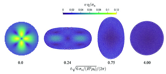
Figure 1. Oscillation of a free droplet with a divergence-free initial velocity field. The normalized velocity magnitude is color-coded. The time is normalized by the oscillation frequency (Equation (52)).

The lateral expansion $L_x$ of the droplet as a function of time is shown in Figure 2. The regular oscillation with decay in amplitude due to viscous dissipation is clearly perceptible.

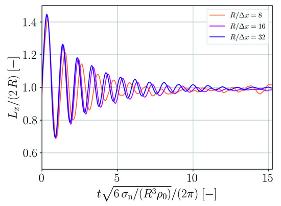
Figure 2. Normalized lateral expansion of the oscillating droplet as a function of normalized time for different spatial resolutions.

A Fourier analysis is carried out in order to assess the oscillation behavior in more detail. The Fourier transform of the droplet expansion, $\mathcal{F}\left(L_x\right)$, is shown in Figure 3 as a function of frequency $f_{\mathrm{sim}}$. For the coarsest spatial resolution, the oscillation is too slow. However, for the two finer resolutions the main frequency peak is in good agreement with the theoretical prediction given by Equation (52).

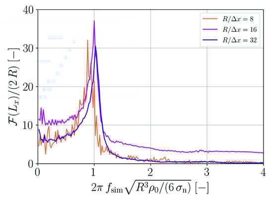
Figure 3. Fourier analysis of the droplet oscillation shown in Figure 2.

3.2. Droplet Formation

The second benchmark is the formation of a droplet from an initial square arrangement of SPH particles as proposed by Adami et al. [6]. The edge length of the square is $L=6\mathrm{m}\mathrm{m}$ and resolutions between 15 and 60 particles per edge length are used yielding a particle spacing between $\Delta x=400 \mathsf{\mu }\mathrm{m}$ and $\Delta x=100 \mathsf{\mu }\mathrm{m}$. Figure 4 shows a sequence of characteristic simulation snapshots using ${60}^2$ particles.

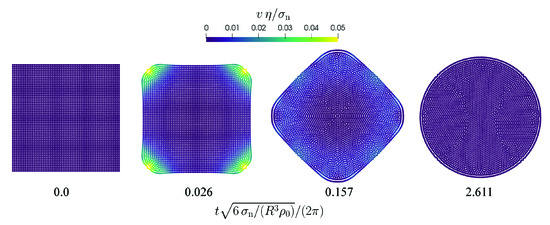
Figure 4. Formation of a droplet from a square under the influence of surface tension. The normalized velocity magnitude is color-coded. The time is normalized using a characteristic oscillation frequency according to Equation (52).

The temporal evolution of the two-dimensional kinetic energy of the droplet for the different spatial resolutions is shown in Figure 5. Following a sharp initial increase of kinetic energy, a decay can be observed for all cases. The decay amounts to about three orders of magnitude for the coarsest resolution while it amounts to more than five orders of magnitude for the finest resolution.

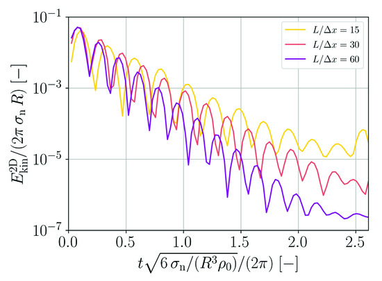
Figure 5. Normalized 2D kinetic energy as a function of normalized time for different spatial resolutions of droplets forming from an initial square patch.

The pressure profile in the eventually formed droplet is evaluated using the SPH approximation according to Equation (9). The results are shown in Figure 6. The finer the spatial resolution the better is the pressure jump at the droplet surface approximated. The agreement with the Young–Laplace equation,

$$P={\sigma }_{\mathrm{n}}/R={\sigma }_{\mathrm{n}}\sqrt{\pi }/L,$$

(53)

which relates the pressure P in the droplet to its radius R, also gets better for finer spatial resolutions.

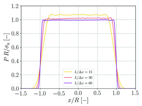
Figure 6. Pressure distribution in the formed droplet as a function of the lateral coordinate at $y=0$ for different spatial resolutions.

The convergence of the numerical solution $P_{\mathrm{sim}}$ with respect to the theoretical result $P_{\mathrm{theo}}$ for the pressure in the droplet is analyzed in Figure 7. It can be observed that the convergence behavior is significantly better than linear and only slightly worse than quadratic.

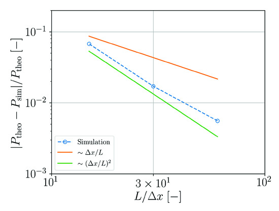
Figure 7. Relative error of the numerically predicted pressure in the droplet as a function of the spatial resolution.

As a final test, the Young–Laplace scaling with R or L, respectively, is tested. In this case, L is increased by a factor of 10 or decreased by a factor of $0.1$ but the particle number of ${30}^2$ is kept constant. The droplet radius of the reference case is referred to as $R_0$. Figure 8 shows that the Young–Laplace scaling is well reproduced.

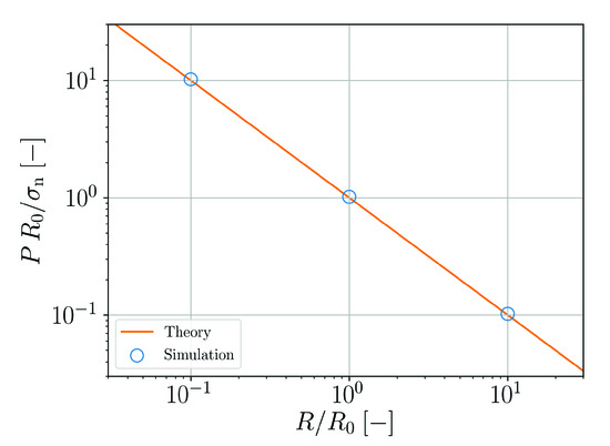
Figure 8. Young–Laplace scaling (Equation (53)) of the normalized droplet pressure as function of the normalized droplet radius.

3.3. Horizontal Substrate Wetting

The third benchmark assesses the wetting behavior of the model similarly to [8]. An initial circular droplet of particles with a radius of $R=3 \mathrm{m}\mathrm{m}$ is placed directly above a planar substrate. The contact angle parameter is varied between $\theta =20{}^{\circ }$ and $\theta =160{}^{\circ }$. No gravity is applied is order to compare the results with simple analytical solutions. Gravity, of course, would have an effect on a droplet of this size. The resulting droplet shapes on the substrate are shown in Figure 9 for a particle spacing of $\Delta x=100 \mathsf{\mu }\mathrm{m}$.

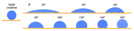
Figure 9. Initial setup and final states of wetting of a substrate for varied numerical contact angle parameter $\theta$.

The predictive quality of these simulations is analyzed by measuring the equilibrium height $H_{\mathrm{eq}}$ and base diameter $D_{\mathrm{eq}}$ of the resulting droplets and comparing them with the analytical results

$$H_{\mathrm{eq}}=(1-cos\theta )\sqrt{\frac{\pi R^2}{\theta -sin\theta cos\theta }}$$

(54)

and

$$D_{\mathrm{eq}}=2sin\theta \sqrt{\frac{\pi R^2}{\theta -sin\theta cos\theta }}.$$

(55)

Figure 10 shows the according simulation results in comparison to the theoretical predictions. The non-trivial shape of both analytical functions is well reproduced up to a contact angle of $\theta =100{}^{\circ }$. Noticeable deviations occur for larger contact angles and the error increases with increasing contact angle.

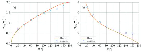
Figure 10. Comparison of simulation results and theory for the wetting of a planar substrate. (a) Normalized droplet height as a function of contact angle parameter. (b) Normalized droplet base diameter as a function of contact angle parameter.

3.4. Vertical Plate Wetting

As fourth benchmark, the wetting of a vertically oriented plate immersed into a fluid is studied. The system is $15 \mathrm{m}\mathrm{m}$ wide with periodic boundary conditions in lateral direction. The initial fluid filling height is $4 \mathrm{m}\mathrm{m}$. A vertical plate is immersed into the fluid down to a distance of $1.5 \mathrm{m}\mathrm{m}$ from the ground. The acceleration of gravity acts in downward direction and the contact angle is varied between $\theta =30{}^{\circ }$ and $\theta =150{}^{\circ }$. A particle spacing of $\Delta x=25 \mathsf{\mu }\mathrm{m}$ is used. Figure 11 shows simulation snapshots after the terminal height of capillary rise or depression, respectively, is reached.

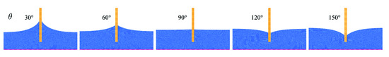
Figure 11. Final states of wetting of a vertical plate for varied numerical contact angle parameter $\theta$.

The accuracy of the simulations is evaluated by comparing the contact angle $\theta$ which enters the numerical model via Equations (39) and (42) with the effective, measured wetting angle with respect to the plate. Figure 12 shows that up to $\theta =90{}^{\circ }$ the agreement is very good. For larger contact angles deviations become more pronounced similarly to the horizontal substrate wetting case in Section 3.3.

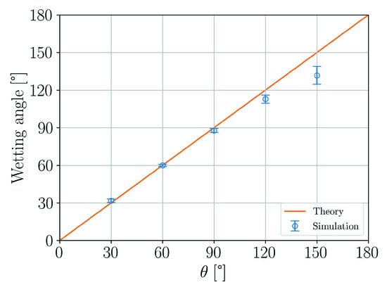
Figure 12. Comparison of simulation results and theory for the wetting of a vertical plate.

3.5. Flow between Parallel Plates

In the fifth benchmark the steady-state flow of a fluid column between parallel plates is analyzed [26]. The length of the column is $h_0=10 \mathrm{c}\mathrm{m}$ and distance of the plates is either $L=0.5 \mathrm{m}\mathrm{m}$ or $L=1 \mathrm{m}\mathrm{m}$. The spatial resolution is $\Delta x=25 \mathsf{\mu }\mathrm{m}$. Different pressure profiles and steady-state velocities of the fluid column are enforced by variation of the advancing contact angle ${\theta }_{\mathrm{adv}}$ and the receding contact angle ${\theta }_{\mathrm{rec}}$ shown in Figure 13.

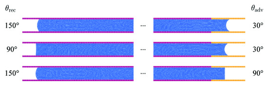
Figure 13. Variation of advancing and receding contact angle for flow between parallel plates.

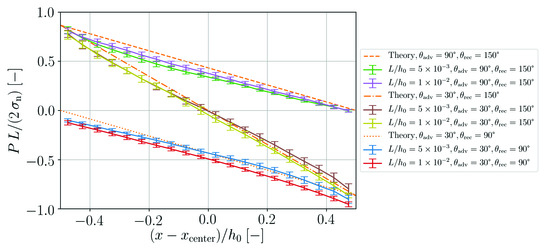
The pressure at the advancing end of the fluid column is given by

$$P_{\mathrm{adv}}=-\frac{2{\sigma }_{\mathrm{n}}cos{\theta }_{\mathrm{adv}}}{L}$$

(56)

and at the receding end of the fluid column by

$$P_{\mathrm{rec}}=-\frac{2{\sigma }_{\mathrm{n}}cos{\theta }_{\mathrm{rec}}}{L}.$$

(57)

An overview of the pressure drop along the fluid column for all simulated cases in comparison to the theory is presented in Figure 14. The obtained pressure profiles are generally in agreement with the analytical predictions. Yet, some finite curvature can be observed in the simulation results while the pressure gradient should be constant in theory.

Figure 14. Normalized pressure as a function of normalized position along the fluid column from numerical simulations and according to theory (Equations (56) and (57)).

The average steady-state velocity of the fluid in the channel is

$$⟨v⟩=\frac{L{\sigma }_{\mathrm{n}}}{6h_0\eta }(cos{\theta }_{\mathrm{adv}}-cos{\theta }_{\mathrm{rec}}).$$

(58)

This theoretical prediction is compared to the simulation results in Figure 15. Within the error bars of the simulation, which represent one standard deviation, agreement with the theory is obtained. Note that in order to obtain stable simulations for this benchmark case it is necessary to increase the numerical speed of sound to $s=30 \mathrm{m}\mathrm{s}{}^{-1}$. For smaller values of s, fragmentation of the particle arrangement in the vicinity of the concave surface is observed. This phenomenon is discussed in Section 4.

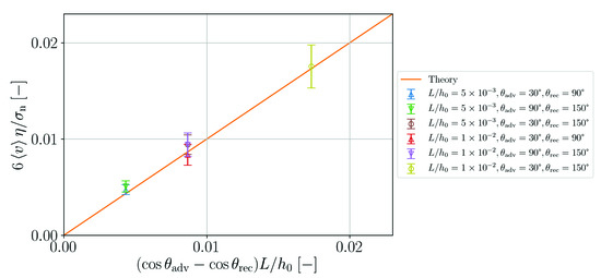
Figure 15. Normalized velocity as function of normalized pressure gradient in the simulations and according to theory (Equation (58)).

3.6. Flow into a Nozzle

The sixth benchmark is similar to the previous one with the difference that the parallel plates are attached to a fluid reservoir resulting in a nozzle geometry. The distance of the parallel plates is either $L=0.5 \mathrm{m}\mathrm{m}$ or $L=1 \mathrm{m}\mathrm{m}$ and the spatial resolution is $\Delta x=25 \mathsf{\mu }\mathrm{m}$. The capillary action of the surface tension with a contact angle $\theta =30{}^{\circ }$ causes the fluid from the reservoir to penetrate the space between the parallel plates. The rise velocity of the fluid decreases over time as shown in Figure 16.

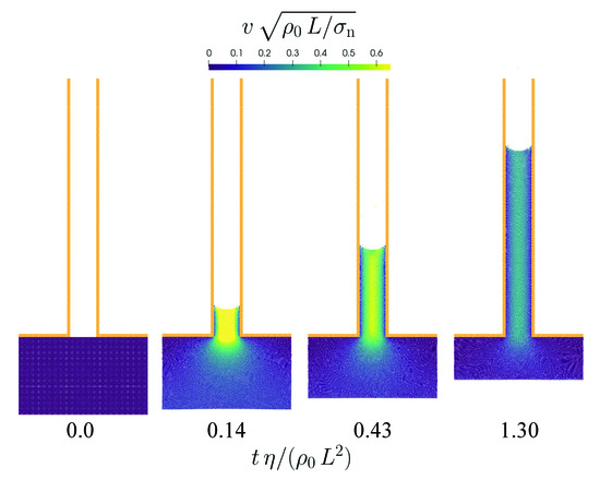
Figure 16. Flow from a reservoir into a nozzle formed by parallel plates. The normalized velocity magnitude is color-coded. The time is normalized using a Reynolds number.

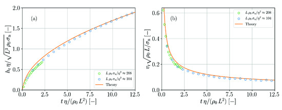
The rise height $h_{\mathrm{r}}$ of the fluid column between the plates and the average rise velocity $v_{\mathrm{r}}$ are obtained by solving the set of differential equations [44]

$$\begin{array}{ccc}\hfill \frac{\mathrm{d}}{\mathrm{d}t}\left(h_{\mathrm{r}}{v}_{\mathrm{r}}\right)& =& -h_{\mathrm{r}}{v}_{\mathrm{r}}\frac{12\eta }{{\rho }_0{L}^2}+\frac{2{\sigma }_{\mathrm{n}}cos\theta }{{\rho }_{0}L},\hfill \end{array}$$

(59)

$$\begin{array}{ccc}\hfill \frac{\mathrm{d}}{\mathrm{d}t}{h}_{\mathrm{r}}& =& v_{\mathrm{r}}.\hfill \end{array}$$

(60)

The according solutions are explicitly given by

$$h_{\mathrm{r}}\left(t\right)=\frac{\sqrt{L^3{\rho }_0{\sigma }_{\mathrm{n}}cos\theta }}{6\eta }\sqrt{\frac{12\eta t}{{\rho }_0{L}^2}+exp\left(-\frac{12\eta t}{{\rho }_0{L}^2}\right)-1}$$

(61)

and

$$v_{\mathrm{r}}\left(t\right)=\sqrt{\frac{{\sigma }_{\mathrm{n}}cos\theta }{{\rho }_{0}L}}\frac{1-exp\left(-\frac{12\eta t}{{\rho }_0{L}^2}\right)}{\sqrt{\frac{12\eta t}{{\rho }_0{L}^2}+exp\left(-\frac{12\eta t}{{\rho }_0{L}^2}\right)-1}}.$$

(62)

These theoretical predictions are compared with the data obtained from the numerical simulations in Figure 17. The transient behavior of both height and velocity are satisfactorily reproduced in the simulations although the actual values are systematically underestimated to a small extent. Note that in order to obtain stable simulations for this benchmark case it is necessary to increase the numerical speed of sound to $s=50 \mathrm{m}\mathrm{s}{}^{-1}$. The reason for this is the avoidance of fragmentation close to the surface similarly to the case in Section 3.5. The even higher speed of sound in this case is required because of the strong acceleration during the initial phase of the flow into the nozzle.

Figure 17. Flow into a nozzle. Normalized rise height (a) and normalized rise velocity (b) as functions of normalized time in simulations and according to theory (Equations (61) and (62)).

3.7. Marangoni Flow

The seventh benchmark focuses on the effect of a surface tension gradient caused by a temperature gradient [9]. A fluid initially rests in a basin of $L=10 \mathrm{m}\mathrm{m}$ width. The left wall of the basin has a constant temperature of $T_{\min }=300 \mathrm{K}$ and the right wall a constant temperature of $T_{\max }=T_{\min }+\Delta T=400 \mathrm{K}$. The fluid temperature initially describes a linear profile interpolating between the values of the walls. The basin bottom is adiabatic. The specific heat capacity of the fluid is $c=1000 \mathrm{J}\mathrm{k}\mathrm{g}{}^{-1}\mathrm{K}{}^{-1}$, the thermal conductivity is $k=10 \mathrm{W}\mathrm{m}{}^{-1}\mathrm{K}{}^{-1}$ and ${\sigma }_{\mathrm{t}}=-1 \mathrm{m}\mathrm{N}\mathrm{m}{}^{-1}\mathrm{K}{}^{-1}$. The particle spacing is varied between $\Delta x=100 \mathsf{\mu }\mathrm{m}$ and $\Delta x=400 \mathsf{\mu }\mathrm{m}$. The contact angle with respect to both side walls is $\theta =90{}^{\circ }$.

Images from the simulation using the spatial resolution $L/\Delta x=100$ are displayed in Figure 18. The fluid strongly rises on the left wall due to the Marangoni effect which drives the fluid at the surface from the warm region towards the cold region. The last snapshot shows the steady state where an eddy has formed below the surface.

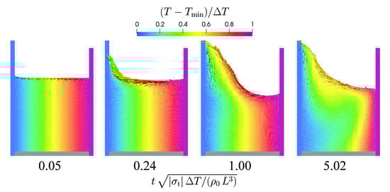
Figure 18. Flow in a basin driven by Marangoni surface current. The normalized temperature is color-coded and the size of the velocity vectors is proportional to the velocity magnitude. The time is normalized by a characteristic Marangoni time scale.

The model is quantitatively assessed by evaluating the Marangoni tension at the surface at the beginning of the simulation using different spatial resolutions as well as different ratios of smoothing length and particle spacing. For this purpose, the tangential volumetric surface force (Equation (6)) is evaluated using SPH interpolation and then integrated along a line perpendicular to the surface. The result $\tau$ should be equal to $|{\sigma }_{\mathrm{t}}{\nabla }_{\mathrm{S}}T|=10 \mathrm{Pa}$. Figure 19 shows that the theoretical result is met for all studied resolutions and smoothing length ratios.

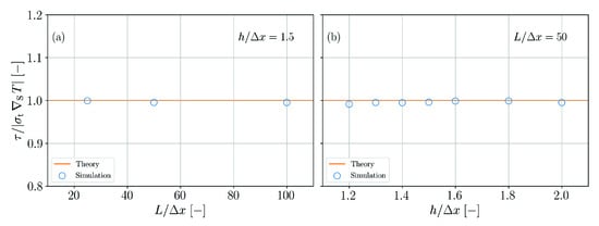
Figure 19. Tangential surface tension induced by temperature gradient. Normalized tension as a function of the spatial resolution (a) and as a function of the normalized smoothing length (b).

3.8. Plate with Double-Sided Heat Transfer

The eighth to eleventh benchmark case do not involve any fluid flow but assess the predictive quality of the thermal boundary conditions at the surface as introduced in Section 2.2.4. A convenient parameter for these cases is the thermal diffusivity, $a=k/\left({\rho }_{0}c\right)$, as it allows to normalize the time and a characteristic length scale in terms of a Fourier number. In all of these four cases the thermal conductivity is $k=1 \mathrm{W}\mathrm{m}{}^{-1}\mathrm{K}{}^{-1}$, the specific heat capacity is $c=100 \mathrm{J}\mathrm{k}\mathrm{g}{}^{-1}\mathrm{K}{}^{-1}$ and the density is ${\rho }_0=7800 \mathrm{k}\mathrm{g}{\mathrm{m}}^{-3}$.

As eighth benchmark an infinite plate with heat transfer on both surfaces is analyzed. The plate thickness is $2L=2 \mathrm{m}\mathrm{m}$ and its initial temperature is $T_0=300 \mathrm{K}$. The heat transfer coefficient is $f=1\times {10}^4 \mathrm{W}{\mathrm{m}}^{-2}\mathrm{K}{}^{-1}$ and the ambient temperature is $T_{\mathrm{a}}=400 \mathrm{K}$.

The analytical solution for this case is given by the series

$$\frac{T(x,t)-T_0}{T_{\mathrm{a}}-T_0}=1-2\sum _{n=1}^{\infty }\frac{sin\left({\gamma }_n\right)cos({\gamma }_{n}x/L)exp(-{\gamma }_n^{2}at/L^2)}{{\gamma }_n+sin\left({\gamma }_n\right)cos\left({\gamma }_n\right)},$$

(63)

where ${\gamma }_n$ is the nth root of the implicit equation

$$\frac{fL}{k}={\gamma }_{n}tan\left({\gamma }_n\right).$$

(64)

The solution is calculated up to $n_{\max }=500$ and compared with the simulation results for different spatial resolutions in Figure 20. While for the lowest spatial resolution the transient temperature is overestimated, differences between theory and simulation vanish for a sufficiently fine resolution.

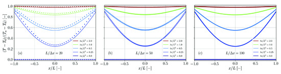
Figure 20. Comparison of simulation results (dots) and analytical solution (solid lines, Equation (63)) for the temperature distribution in a plate with double-sided heat transfer. The spatial resolution is varied between $L/\Delta x=20$ (a), $L/\Delta x=50$ (b) and $L/\Delta x=100$ (c).

3.9. Plate with Double-Sided Heat Flux

The ninth benchmark is similar to the eighth one with the difference that instead of heat transfer a heat flux $q=1\times {10}^4 \mathrm{W}{\mathrm{m}}^{-2}$ is prescribed at both surfaces of the plate.

The solution for this situation is given by

$$\frac{(T(x,t)-T_0)k}{qL}=\frac{at}{L^2}+\frac{x^2}{2L^2}-\frac{1}{6}-2\sum _{n=1}^{\infty }\frac{{(-1)}^n}{{\gamma }_n^2}cos({\gamma }_{n}x/L)exp(-{\gamma }_n^{2}at/L^2),$$

(65)

with ${\gamma }_n$ defined by

$${\gamma }_n=n\pi .$$

(66)

Again, the series is evaluated up to $n_{\max }=500$ and simulation and theory are compared in Figure 21 for different spatial resolutions. Perfect agreement is found independent of the actual resolution.

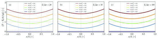
Figure 21. Comparison of simulation results (dots) and analytical solution (solid lines, Equation (65)) for the temperature distribution in a plate with double-sided heat flux. The spatial resolution is varied between $L/\Delta x=20$ (a), $L/\Delta x=50$ (b) and $L/\Delta x=100$ (c).

3.10. Plate with Heat Transfer and Heat Flux

The tenth benchmark is a combination of the two previous ones. An infinite plate of thickness $L=1\mathrm{m}\mathrm{m}$ experiences heat transfer with $f=1\times {10}^4 \mathrm{W}{\mathrm{m}}^{-2}\mathrm{K}{}^{-1}$ and $T_{\mathrm{a}}=300 \mathrm{K}$ at $x/L=0$ and heat flux with $q=1\times {10}^4 \mathrm{W}{\mathrm{m}}^{-2}$ at $x/L=1$. The initial temperature of the plate is $T_0=T_{\mathrm{a}}$.

The analytical series solution is given by

$$\frac{(T(x,t)-T_0)f}{q}=1+\frac{fx}{k}-\sum _{n=1}^{\infty }\left(cos({\gamma }_{n}x/L)+\frac{fL}{k{\gamma }_n}sin({\gamma }_{n}x/L)\right)\frac{2sin\left({\gamma }_n\right)exp(-{\gamma }_n^{2}at/L^2)}{{\gamma }_n+sin\left({\gamma }_n\right)cos\left({\gamma }_n\right)},$$

(67)

with the roots ${\gamma }_n$ given by

$$\frac{fL}{k}={\gamma }_{n}tan\left({\gamma }_n\right).$$

(68)

A comparison between simulation and theory ($n_{\max }=500$) for different spatial resolutions is provided in Figure 22. For too coarse resolutions and Fourier numbers $ta/L^2\gtrsim 1$ the temperature is underestimated by the simulation. Yet, similarly to the benchmark case with double-sided heat transfer (Section 3.8), the analytical solution gets better approximated with finer spatial resolution.

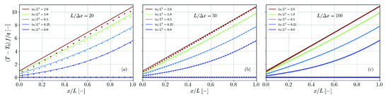
Figure 22. Comparison of simulation results (dots) and analytical solution (solid lines, Equation (67)) for the temperature distribution in a plate with heat transfer and heat flux. The spatial resolution is varied between $L/\Delta x=20$ (a), $L/\Delta x=50$ (b) and $L/\Delta x=100$ (c).

3.11. Rod with Heat Flux

In the eleventh benchmark an infinite rod of radius $R=1 \mathrm{m}\mathrm{m}$ and initial temperature $T_0=300 \mathrm{K}$ is heated by the surface heat flux $q=1\times {10}^4 \mathrm{W}{\mathrm{m}}^{-2}$.

The according analytical solution for the temperature distribution along the radial coordinate r is given by

$$\frac{(T(r,t)-T_0)k}{qR}=\frac{2at}{R^2}+\frac{r^2}{2R^2}-\frac{1}{4}-2\sum _{n=1}^{\infty }\frac{J_0({\gamma }_{n}r/R)exp(-{\gamma }_n^{2}at/R^2)}{{\gamma }_n^2{J}_0\left({\gamma }_n\right)},$$

(69)

with the nth root ${\gamma }_n$ given by

$$J_1\left({\gamma }_n\right)=0.$$

(70)

Due to the rotational symmetry of this benchmark case, the Bessel functions of the first kind $J_0$ and $J_1$ appear in the solution. The comparison between the simulation results and the analytical solution in Figure 23 reveals that the temperature is underestimated for too coarse spatial resolutions. However, for finer resolution the analytical result is well predicted.

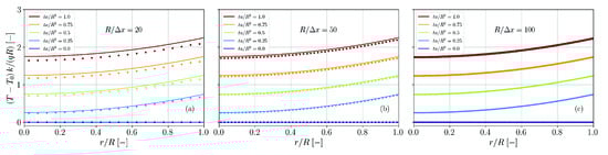
Figure 23. Comparison of simulation results (dots) and analytical solution (solid lines, Equation (69)) for the temperature distribution in a rod with surface heat flux. The spatial resolution is varied between $R/\Delta x=20$ (a), $R/\Delta x=50$ (b) and $R/\Delta x=100$ (c).

For this case, the accuracy of the surface heat transfer in the simulation is assessed by evaluating the rate of change of thermal energy in the simulation. As heat transfer is the only active heating mechanism, the rate of thermal energy change should be directly proportional to the applied heat flux. An according convergence analysis is plotted in Figure 24. The effective heat flux in the simulation converges approximately linear with the spatial resolution.

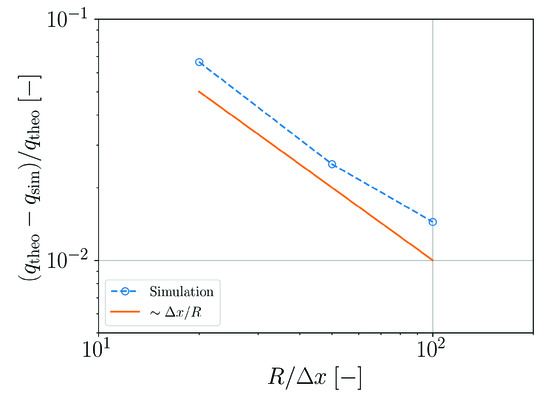
Figure 24. Relative error of the numerically predicted heat flux in a rod as a function of the spatial resolution.

3.12. Droplet Deformation and Splitting

The twelfth case is intended to study the usage of the presented model in a more complex three-dimensional situation. A droplet of fluid with a diameter of $1 \mathrm{m}\mathrm{m}$ is discretized using $\Delta x=20 \mathsf{\mu }\mathrm{m}$. The droplet floats above a substrate initially. Gravity pushes the droplet onto the substrate which consists of hydrophilic regions with a contact angle of $\theta =45{}^{\circ }$ and hydrophobic regions with a contact angle of $\theta =135{}^{\circ }$. Two different substrates are used. One is composed of square regions having a certain contact angle. The other substrate consists of striped regions with a width of $400 \mathsf{\mu }\mathrm{m}$. The numerical speed of sound in the simulation is $s=3 \mathrm{m}\mathrm{s}{}^{-1}$. Figure 25 shows the temporal evolution of the fluid droplet on both substrates. For the square regions, the wetting and de-wetting behavior leads eventually to a splitting of the droplet into two. For the striped regions, the droplet does not split up but ends up with a very peculiar shape of its perimeter.

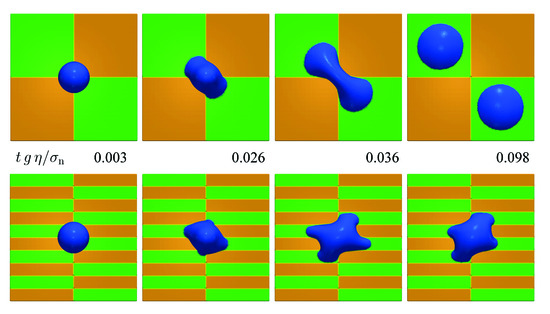
Figure 25. Wetting behavior of a droplet on substrates composed of hydrophilic regions (green, $\theta =45{}^{\circ }$) and hydrophobic regions (orange, $\theta =135{}^{\circ }$).

3.13. Thermo-Visco-Capillary Droplet Coalescence

The thirteenth and final case contains the most complex simulation setup. Two droplets of fluid with diameters of $1 \mathrm{m}\mathrm{m}$ are discretized using $\Delta x=20 \mathsf{\mu }\mathrm{m}$. The droplets touch a substrate below as well as each other initially. Gravity acts normal to the substrate surface. The fluid has an initial temperature of $T_{\min }=300 \mathrm{K}$ and the substrate a constant temperature of $T_{\max }=T_{\min }+\Delta T=500 \mathrm{K}$. The specific heat capacity of the fluid is $c=1000 \mathrm{J}\mathrm{k}\mathrm{g}{}^{-1}\mathrm{K}{}^{-1}$ and the thermal conductivity of both fluid and substrate is $k=10 \mathrm{W}\mathrm{m}{}^{-1}\mathrm{K}{}^{-1}$. The surface tension of the fluid is

$${\sigma }_{\mathrm{n}}\left(T\right)={\tilde{\sigma }}_{\mathrm{n}}+{\sigma }_{\mathrm{t}}(T-T_{\min })$$

(71)

with ${\tilde{\sigma }}_{\mathrm{n}}=48.4 \mathrm{m}\mathrm{N}\mathrm{m}{}^{-1}$ and ${\sigma }_{\mathrm{t}}=-0.2 \mathrm{m}\mathrm{N}\mathrm{m}{}^{-1}\mathrm{K}{}^{-1}$. The contact angle with respect to the substrate is $\theta =45{}^{\circ }$. The ambient temperature is $T_{\mathrm{a}}=T_{\min }$ and the fluid is cooled by surface heat transfer with $f=1\times {10}^2 \mathrm{W}\mathrm{m}{}^{-2}\mathrm{K}{}^{-1}$ and by radiation with $\epsilon =0.5$. The viscosity of the fluid is temperature-dependent in the form of an Arrhenius relation,

$$\eta \left(T\right)=\tilde{\eta }exp\left(\frac{E_{\mathrm{a}}}{R}\left(\frac{1}{T}-\frac{1}{T_{\min }}\right)\right),$$

(72)

with $\tilde{\eta }=16.1 \mathrm{m}\mathrm{Pa}\mathrm{s}$, the activation energy $E_{\mathrm{a}}=1\times {10}^4 \mathrm{J}\mathrm{mol}{}^{-1}$ and the universal gas constant $R=8.314 \mathrm{J}\mathrm{mol}{}^{-1}\mathrm{K}{}^{-1}$. The numerical speed of sound is $s=3 \mathrm{m}\mathrm{s}{}^{-1}$. The thermo-visco-capillary coalescence behavior of the droplets is shown from different perspectives in Figure 26.

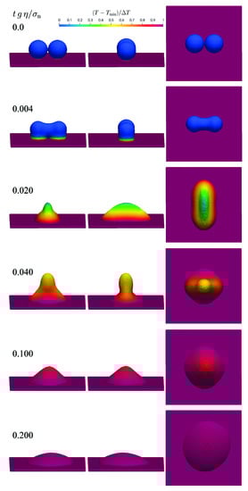
Figure 26. Coalescence of two droplets under the influences of temperature-dependent viscosity and surface tension.

4. Discussion

The presented consistent modeling of thermo-capillary effects and thermal boundary conditions within the SPH method could be verified and validated by the extensive analyses in Section 3. In the following, we would like to address some details which could be highlighted by the analyses.

For free droplets, the visco-capillary oscillation frequency and the Laplace pressure are adequately reproduced by the simulations with sufficient spatial resolution. For the Laplace pressure, a near quadratic convergence with spatial resolution has been found. At the finest resolution used, the relative error is less than ${10}^{-2}$, which is typically an acceptable tolerance for SPH simulations [2].

The investigations on static wetting have shown that contact angles up to $\theta \approx 100{}^{\circ }$ are well reproduced in the simulation. Larger contact angles are increasingly poorly reproduced. A comparable observation was made by Breinlinger et al. [8]. This is apparently a systematic weakness of the submodel for imprinting the desired contact angle in Section 2.2.11. The reason for this is that in the approach used to determine the free surface and the quantities derived from it, the fluid and the substrate are initially considered as a common phase. As a result, it is not possible to identify free surfaces that are only separated by small gaps. However, precisely this situation exists in the case of large contact angles. Alternatively, the fluid and the substrate could be considered as distinct phases from the beginning. In that case, however, the reproduction of small contact angles would become increasingly inaccurate, which has been observed in corresponding tests.

In the dynamic wetting scenarios, a satisfactory overall agreement of the simulation with theoretical predictions for the pressure and velocity has been observed. A slight, systematic deviation in the dynamic wetting case in Section 3.6 can be explained by the fact that the momentum of the reservoir is not considered in the respective balance equation (Equation (59)). The strong tensile stresses caused by the surface tension in the dynamic wetting scenarios are seen as the reason why it is necessary to slightly increase the numerical speed of sound in these cases. Without such an increase, fragmentation of the particles near the surface has been observed. In this context, the used approach of a surface delta function based on the minimum eigenvalue $\lambda$ of the inverse renormalization tensor has proved to be helpful. As shown in the Appendix A, the surface delta function is more evenly distributed among the particle layers on the surface than when using a delta function which is based only on the kernel gradient. This attenuates the tensile forces acting on the individual particles, which helps to stabilize the simulation. The use of a weak artificial viscosity and the viscosity formulation of Sigalotti et al. [38] have also proved to stabilize the dynamic wetting scenarios.

A fundamental strength of the presented model is that only one phase has to be modeled. This saves computational time, since especially for systems consisting of a fluid and a gas, the low density of the gas requires a very small time step, as shown by Colagrossi and Landrini [45]. However, even the presented model may require a relatively small time step due to a high numerical speed of sound, as described in the previous paragraph. For such a situation, the use of an implicit SPH formulation can be useful, such as the ones used by Nair and Pöschel [31] or Fürstenau et al. [20] in the context of capillary phenomena.

The investigations on the heat transfer boundary condition have shown that agreements with analytical results are obtained by simulations with sufficiently fine spatial resolution. In the case of a pure heat flux boundary condition on a flat surface, excellent accuracy of the numerical simulations has been found regardless of the spatial resolution. This can probably be attributed to the fact that the heat input is independent of the temperature computed in the numerical simulation. In the case of a curved surface, a linear convergence of the relative error of the heat flux with the spatial discretization could be determined. This convergence behavior can be considered a measure of how well the surface delta function describes a curved surface.

The two cases in Section 3.12 and Section 3.13 are not intended to validate the model but to provide ideas for application in more complex scenarios. Use cases for thermo-capillary SPH simulations offer, for example, welding processes (Hu and Eberhard [46]) or additive manufacturing processes (Russell et al. [47], Fürstenau et al. [48], Meier et al. [49]). The presented method has already been applied by the author and coworkers to derive universal process maps for laser powder bed fusion of polymers [50].

Based on the identified weakness of the presented model, a more accurate description of large contact angles is considered as a future field of development. In addition, the modeling of dynamic wetting phenomena can be improved by considering the dynamic contact angle as in Huber et al. [11]. A fundamental problem for single-phase models based on the CSF approach is the lack of possibility to formulate the surface tension forces in a momentum-preserving way. As a consequence, sooner or later a non-physical drift of free-floating droplets or of droplets on flat substrates occurs in the simulations. A solution to this problem would be highly desirable in terms of a more universal applicability of the method.

5. Conclusions

The main contributions of the present work are summarized in the following list:

• The surface delta function, surface normal and surface curvature are derived in a consistent manner from the renormalization tensor in single-phase SPH simulations.
• Thermo-capillarity, wetting and thermal boundary conditions are formulated in a uniform way based on these surface properties.
• The quantitative agreement of corresponding simulations with a large number of analytical test cases demonstrates the validity of the presented approach.

References

- Monaghan, J.J. Smoothed Particle Hydrodynamics. Annu. Rev. Astron. Astrophys. 1992, 30, 543–574. [Google Scholar] [CrossRef]
- Monaghan, J.J. Smoothed particle hydrodynamics. Rep. Prog. Phys. 2005, 68, 1703–1759. [Google Scholar] [CrossRef]
- Brackbill, J.U.; Kothe, D.B.; Zemach, C. A continuum method for modeling surface tension. J. Comput. Phys. 1992, 100, 335–354. [Google Scholar] [CrossRef]
- Morris, J.P. Simulating surface tension with smoothed particle hydrodynamics. Int. J. Numer. Methods Fluids 2000, 33, 333–353. [Google Scholar] [CrossRef]
- Hu, X.Y.; Adams, N.A. A multi-phase SPH method for macroscopic and mesoscopic flows. J. Comput. Phys. 2006, 213, 844–861. [Google Scholar] [CrossRef]
- Adami, S.; Hu, X.Y.; Adams, N.A. A new surface-tension formulation for multi-phase SPH using a reproducing divergence approximation. J. Comput. Phys. 2010, 229, 5011–5021. [Google Scholar] [CrossRef]
- Zhang, M. Simulation of surface tension in 2D and 3D with smoothed particle hydrodynamics method. J. Comput. Phys. 2010, 229, 7238–7259. [Google Scholar] [CrossRef]
- Breinlinger, T.; Polfer, P.; Hashibon, A.; Kraft, T. Surface tension and wetting effects with smoothed particle hydrodynamics. J. Comput. Phys. 2013, 243, 14–27. [Google Scholar] [CrossRef]
- Tong, M.; Browne, D.J. An incompressible multi-phase smoothed particle hydrodynamics (SPH) method for modelling thermocapillary flow. Int. J. Heat Mass Transf. 2014, 73, 284–292. [Google Scholar] [CrossRef]
- Yeganehdoust, F.; Yaghoubi, M.; Emdad, H.; Ordoubadi, M. Numerical study of multiphase droplet dynamics and contact angles by smoothed particle hydrodynamics. Appl. Math. Model. 2016, 40, 8493–8512. [Google Scholar] [CrossRef]
- Huber, M.; Keller, F.; Säckel, W.; Hirschler, M.; Kunz, P.; Hassanizadeh, S.M.; Nieken, U. On the physically based modeling of surface tension and moving contact lines with dynamic contact angles on the continuum scale. J. Comput. Phys. 2016, 310, 459–477. [Google Scholar] [CrossRef]
- Ordoubadi, M.; Yaghoubi, M.; Yeganehdoust, F. Surface tension simulation of free surface flows using smoothed particle hydrodynamics. Sci. Iran. 2017, 24, 2019–2033. [Google Scholar] [CrossRef][Green Version]
- Lee, E.S.; Moulinec, C.; Xu, R.; Violeau, D.; Laurence, D.; Stansby, P. Comparisons of weakly compressible and truly incompressible algorithms for the SPH mesh free particle method. J. Comput. Phys. 2008, 227, 8417–8436. [Google Scholar] [CrossRef]
- Hirschler, M.; Oger, G.; Nieken, U.; Le Touzé, D. Modeling of droplet collisions using Smoothed Particle Hydrodynamics. Int. J. Multiph. Flow 2017, 95, 175–187. [Google Scholar] [CrossRef]
- Bonet, J.; Lok, T.S.L. Variational and momentum preservation aspects of Smooth Particle Hydrodynamic formulations. Comput. Methods Appl. Mech. Eng. 1999, 180, 97–115. [Google Scholar] [CrossRef]
- Krimi, A.; Rezoug, M.; Khelladi, S.; Nogueira, X.; Deligant, M.; Ramírez, L. Smoothed Particle Hydrodynamics: A consistent model for interfacial multiphase fluid flow simulations. J. Comput. Phys. 2018, 358, 53–87. [Google Scholar] [CrossRef]
- Hopp-Hirschler, M.; Shadloo, M.S.; Nieken, U. A Smoothed Particle Hydrodynamics approach for thermo-capillary flows. Comput. Fluids 2018, 176, 1–19. [Google Scholar] [CrossRef]
- Xu, R.; Stansby, P.; Laurence, D. Accuracy and stability in incompressible SPH (ISPH) based on the projection method and a new approach. J. Comput. Phys. 2009, 228, 6703–6725. [Google Scholar] [CrossRef]
- Lin, Y.; Liu, G.R.; Wang, G. A particle-based free surface detection method and its application to the surface tension effects simulation in smoothed particle hydrodynamics (SPH). J. Comput. Phys. 2019, 383, 196–206. [Google Scholar] [CrossRef]
- Fürstenau, J.P.; Weißenfels, C.; Wriggers, P. Free surface tension in incompressible smoothed particle hydrodynamcis (ISPH). Comput. Mech. 2020, 65, 487–502. [Google Scholar] [CrossRef]
- Liu, X.; Morita, K.; Zhang, S. Machine-learning-based surface tension model for multiphase flow simulation using particle method. Int. J. Numer. Methods Fluids 2021, 93, 356–368. [Google Scholar] [CrossRef]
- Härdi, S.; Schreiner, M.; Janoske, U. On a new algorithm for incorporating the contact angle forces in a simulation using the shallow water equation and smoothed particle hydrodynamics. Comput. Fluids 2021, 215, 104793. [Google Scholar] [CrossRef]
- Liu, W.B.; Ma, D.J.; Zhang, M.Y.; He, A.M.; Liu, N.S.; Wang, P. A new surface tension formulation in smoothed particle hydrodynamics for free-surface flows. J. Comput. Phys. 2021, 439, 110203. [Google Scholar] [CrossRef]
- Sun, P.N.; Colagrossi, A.; Marrone, S.; Zhang, A.M. The δplus-SPH model: Simple procedures for a further improvement of the SPH scheme. Comput. Methods Appl. Mech. Eng. 2017, 315, 25–49. [Google Scholar] [CrossRef]
- Nugent, S.; Posch, H.A. Liquid drops and surface tension with smoothed particle applied mechanics. Phys. Rev. E 2000, 62, 4968–4975. [Google Scholar] [CrossRef] [PubMed]
- Tartakovsky, A.; Meakin, P. Modeling of surface tension and contact angles with smoothed particle hydrodynamics. Phys. Rev. E 2005, 72, 026301. [Google Scholar] [CrossRef]
- Akinci, N.; Akinci, G.; Teschner, M. Versatile surface tension and adhesion for SPH fluids. ACM Trans. Graph. 2013, 32, 1–8. [Google Scholar] [CrossRef]
- Kirkwood, J.G.; Buff, F.P. The Statistical Mechanical Theory of Surface Tension. J. Chem. Phys. 1949, 17, 338–343. [Google Scholar] [CrossRef]
- Marchand, A.; Weijs, J.H.; Snoeijer, J.H.; Andreotti, B. Why is surface tension a force parallel to the interface? Am. J. Phys. 2011, 79, 999–1008. [Google Scholar] [CrossRef]
- Tartakovsky, A.M.; Panchenko, A. Pairwise Force Smoothed Particle Hydrodynamics model for multiphase flow: Surface tension and contact line dynamics. J. Comput. Phys. 2016, 305, 1119–1146. [Google Scholar] [CrossRef]
- Nair, P.; Pöschel, T. Dynamic capillary phenomena using Incompressible SPH. Chem. Eng. Sci. 2018, 176, 192–204. [Google Scholar] [CrossRef]
- Bao, Y.; Li, L.; Shen, L. Modified smoothed particle hydrodynamics approach for modelling dynamic contact angle hysteresis. Acta Mech. Sin. 2019, 35, 472–485. [Google Scholar] [CrossRef]
- Bierwisch, C. A surface tension and wetting model for the δ+-SPH scheme. In Proceedings of the 13th SPHERIC International Workshop, Galway, Ireland, 26–28 June 2018; National University of Ireland Galway: Galway, Ireland, 2018; pp. 95–102. [Google Scholar]
- Marrone, S.; Colagrossi, A.; Le Touzé, D.; Graziani, G. Fast free-surface detection and level-set function definition in SPH solvers. J. Comput. Phys. 2010, 229, 3652–3663. [Google Scholar] [CrossRef]
- Wendland, H. Piecewise polynomial, positive definite and compactly supported radial functions of minimal degree. Adv. Comput. Math. 1995, 4, 389–396. [Google Scholar] [CrossRef]
- Price, D.J. Smoothed particle hydrodynamics and magnetohydrodynamics. J. Comput. Phys. 2012, 231, 759–794. [Google Scholar] [CrossRef]
- Cleary, P.W. Modelling confined multi-material heat and mass flows using SPH. Appl. Math. Model. 1998, 22, 981–993. [Google Scholar] [CrossRef]
- Sigalotti, L.D.G.; Klapp, J.; Sira, E.; Meleán, Y.; Hasmy, A. SPH simulations of time-dependent Poiseuille flow at low Reynolds numbers. J. Comput. Phys. 2003, 191, 622–638. [Google Scholar] [CrossRef]
- Courant, R.; Friedrichs, K.; Lewy, H. Über die partiellen Differenzengleichungen der mathematischen Physik. Math. Ann. 1928, 100, 32–74. [Google Scholar] [CrossRef]
- Morris, J.P.; Fox, P.J.; Zhu, Y. Modeling Low Reynolds Number Incompressible Flows Using SPH. J. Comput. Phys. 1997, 136, 214–226. [Google Scholar] [CrossRef]
- Cleary, P.W.; Monaghan, J.J. Conduction Modelling Using Smoothed Particle Hydrodynamics. J. Comput. Phys. 1999, 148, 227–264. [Google Scholar] [CrossRef]
- Swope, W.C.; Andersen, H.C.; Berens, P.H.; Wilson, K.R. A computer simulation method for the calculation of equilibrium constants for the formation of physical clusters of molecules: Application to small water clusters. J. Chem. Phys. 1982, 76, 637–649. [Google Scholar] [CrossRef]
- SimPARTIX. Available online: https://www.simpartix.com. (accessed on 23 July 2021).
- Zhmud, B.V.; Tiberg, F.; Hallstensson, K. Dynamics of Capillary Rise. J. Colloid Interface Sci. 2000, 228, 263–269. [Google Scholar] [CrossRef] [PubMed]
- Colagrossi, A.; Landrini, M. Numerical simulation of interfacial flows by smoothed particle hydrodynamics. J. Comput. Phys. 2003, 191, 448–475. [Google Scholar] [CrossRef]
- Hu, H.; Eberhard, P. Thermomechanically coupled conduction mode laser welding simulations using smoothed particle hydrodynamics. Comput. Part. Mech. 2017, 4, 473–486. [Google Scholar] [CrossRef]
- Russell, M.A.; Souto-Iglesias, A.; Zohdi, T.I. Numerical simulation of Laser Fusion Additive Manufacturing processes using the SPH method. Comput. Methods Appl. Mech. Eng. 2018, 341, 163–187. [Google Scholar] [CrossRef]
- Fürstenau, J.P.; Wessels, H.; Weißenfels, C.; Wriggers, P. Generating virtual process maps of SLM using powder-scale SPH simulations. Comput. Part. Mech. 2020, 7, 655–677. [Google Scholar] [CrossRef]
- Meier, C.; Fuchs, S.L.; Hart, A.J.; Wall, W.A. A novel smoothed particle hydrodynamics formulation for thermo-capillary phase change problems with focus on metal additive manufacturing melt pool modeling. Comput. Methods Appl. Mech. Eng. 2021, 381, 113812. [Google Scholar] [CrossRef]
- Bierwisch, C.; Mohseni-Mofidi, S.; Dietemann, B.; Grünewald, M.; Rudloff, J.; Lang, M. Universal process diagrams for laser sintering of polymers. Mater. Des. 2021, 199, 109432. [Google Scholar] [CrossRef]
Publisher’s Note: MDPI stays neutral with regard to jurisdictional claims in published maps and institutional affiliations. |
© 2021 by the author. Licensee MDPI, Basel, Switzerland. This article is an open access article distributed under the terms and conditions of the Creative Commons Attribution (CC BY) license (https://creativecommons.org/licenses/by/4.0/).