Comparative Study and Limits of Different Level-Set Formulations for the Modeling of Anisotropic Grain Growth

Abstract

In this study, four different finite element level-set (FE-LS) formulations are compared for the modeling of grain growth in the context of polycrystalline structures and, moreover, two of them are presented for the first time using anisotropic grain boundary (GB) energy and mobility. Mean values and distributions are compared using the four formulations. First, we present the strong and weak formulations for the different models and the crystallographic parameters used at the mesoscopic scale. Second, some Grim Reaper analytical cases are presented and compared with the simulation results, and the evolutions of individual multiple junctions are followed. Additionally, large-scale simulations are presented. Anisotropic GB energy and mobility are respectively defined as functions of the mis-orientation/inclination and disorientation. The evolution of the disorientation distribution function (DDF) is computed, and its evolution is in accordance with prior works. We found that the formulation called “Anisotropic” is the more physical one, but it could be replaced at the mesoscopic scale by an isotropic formulation for simple microstructures presenting an initial Mackenzie-type DDF.

1. Introduction

The study of GB Thermodynamics and Kinetics are two fundamental topics in materials science. The study of thermodynamics provides information about a system at equilibrium; its extrapolation, under the assumption of local equilibrium, provides the basis for kinetic theories. Additionally, kinetics approaches study the evolution of systems out of equilibrium, involving changes in the microstructure. Determining the kinetics of recovery, grain growth (GG), recrystallization, solidification and other metallurgical mechanisms is necessary to predict and optimize material properties [1]. The need for high-performance materials demands a better knowledge and control of the behavior of GBs under thermomechanical loads. This topic became a strong issue of materials science and gave rise to a branch called GB engineering [2].

In the context of GG, the evolution of GB is driven by the reduction of interfacial energy, and its velocity is classically described, at the mesoscopic scale, by the well-known equation ${\displaystyle v=\mu P}$, where ${\displaystyle \mu }$ is the GB mobility and ${\displaystyle P=-\gamma \kappa }$ is the curvature flow driving pressure with ${\displaystyle \gamma }$, the GB energy, and ${\displaystyle \kappa }$, the mean curvature (i.e., the trace of the curvature tensor in 3D). This kinetic equation is a simplification of lower scale phenomena in constant discussions [3,4]. In this case, it constitutes the polycrystalline scale, and in metal forms a state-of-the-art kinematically accepted physical framework. In the discussion of whether this kinetic equation is a reasonable approximation [5] and whether the reduced mobility (${\displaystyle \mu \gamma }$ product) can really be considered as defined by the temperature and macroscopic properties of the interface as mis-orientation and inclination, a clear and univocal answer seems complicated today. First of all, the answer at the few interfaces scale and at the homogenized polycrystal scale can be contradictory as to the statistical effects. Moreover, a bias in the reduced mobility field discussion today lies in the real capacity of full-field methods to take into account a reduced mobility appropriately defined in the 5D space, defined by the mis-orientation and inclination in representative 2D or 3D simulations. As detailed below, such a capacity is typically unclear in the current state-of-the-art. Thus, the discussion between experimental data and anisotropic full-field simulations is to be treated with extreme caution.

If numerical modeling by considering heterogeneous values of GB mobility and GB energy remains a complex discussion, it has in fact been widely studied at the polycrystalline scale with a large variety of numerical approaches: multi phase-field [6,7,8], Monte Carlo [9,10], molecular dynamics [11], orientated tessellation updating method [12], vertex [13], front-tracking Lagrangian or Eulerian formulations in a finite element (FE) context [14,15,16], and level-set (LS) [17,18,19], to cite some examples. During annealing, two properties have been widely studied: the GB energy and mobility. The first models proposed in the literature define the GB mobility and energy as constants, carrying the name of isotropic, [6,9,17,20,21], and this category shows good agreement in terms of mean quantities and distributions; nevertheless, they are restrictive in terms of the grains’ morphology and texture predictions. GB energy and mobility were earlier reported as anisotropic by Smith [22] and Kohara [23]. Hence, the models have evolved in order to reproduce more complex microstructures or local heterogeneities, such as twin boundaries. Heterogeneous models were proposed, in which each boundary has its own energy and mobility [10,18,19,24,25,26,27,28,29,30,31]. For instance, every grain could be related with an orientation, thus the mobility and energy can be computed in terms of the disorientation [7,19], but the mis-orientation axis and inclination dependence are frequently not taken into account. Finally, general frameworks in which the five parameters, mis-orientation, and inclination are discussed have been proposed, and these models could be categorized as fully anisotropic [32,33,34].

However, it must be highlighted that the distinction between 3-parameter and 5-parameter full-field frameworks is not straightforward because of unclear terminology. In the literature, heterogeneous values of GB properties have often been categorized as anisotropic. For instance, in [7,12,29,31,35], heterogeneous GB energy and a constant GB mobility to model polycrystal evolution during GG are considered, and the models are categorized as anisotropic even if it is assumed that the GB energy does not depend on the GB normal direction and the GB mobility is not heterogeneous. In [34], the proposed LS formulation in the context of regular grids includes the effect of anisotropic GB energy into the driving force term (${\displaystyle P}$) using both the effect of the mis-orientation and the inclination in a GB energy gradient. However, the GB energy dependence on the normal direction is defined without inquiring if additional torque terms in the solved equations are negligible or not.

Due to the wide variety of formulations, this paper aims to compare four different formulations within an FE-LS approach. The first is an isotropic formulation frequently used in different contexts, such as GG, recrystallization, and GG with second-phase particles [17,36,37,38,39], referred to as the isotropic model in the following. The second one is a simple extension of the isotropic formulation by considering non-homogeneous values of the reduced mobility. The third formulation was firstly proposed in [26] and extended to polycrystals using different models of GB energy in [19]. The last formulation is based on a more robust thermodynamics and differential geometry framework, but was only applied, as yet, to a bicrystal-like geometry [33]. Another particularity of the discussed approaches is to be usable on unstructured finite element mesh and in the context of large deformations and displacements. The goals of this work are to criticize these existing formulations but also to consider the enrichment of GB mobility in the FE-LS framework. First, some crystallographic definitions, LS treatments, and formulations are introduced in Section 2. In Section 3, simulation results are compared with analytical solutions in the context of simple triple junction geometries. In Section 4, polycrystalline simulations are studied. Mean values and statistical quantities are compared with two different initial textures and using heterogeneous GB energy and mobility. Finally, the last section is dedicated to the inclination dependence discussions.

2. The Numerical Framework

Before formulating the equations related to GG, the constituents of polycrystalline materials and especially GB structures must be defined.

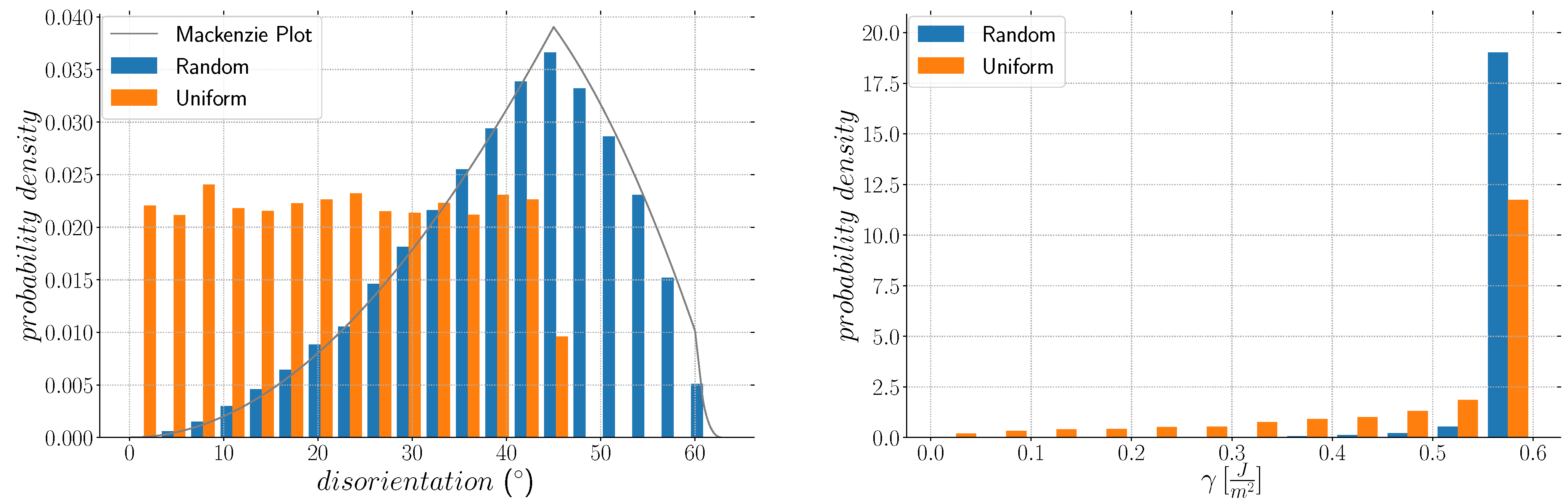
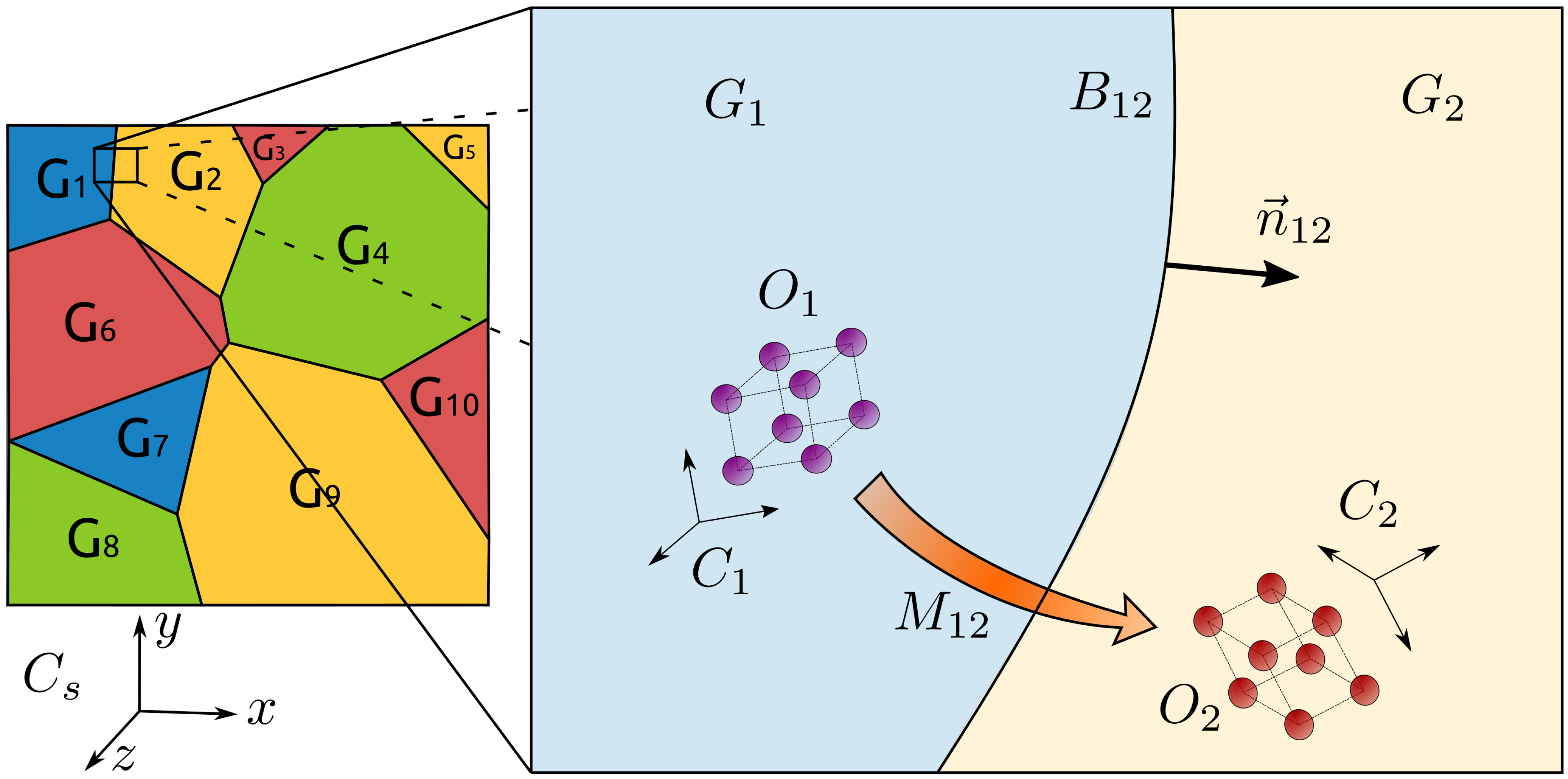
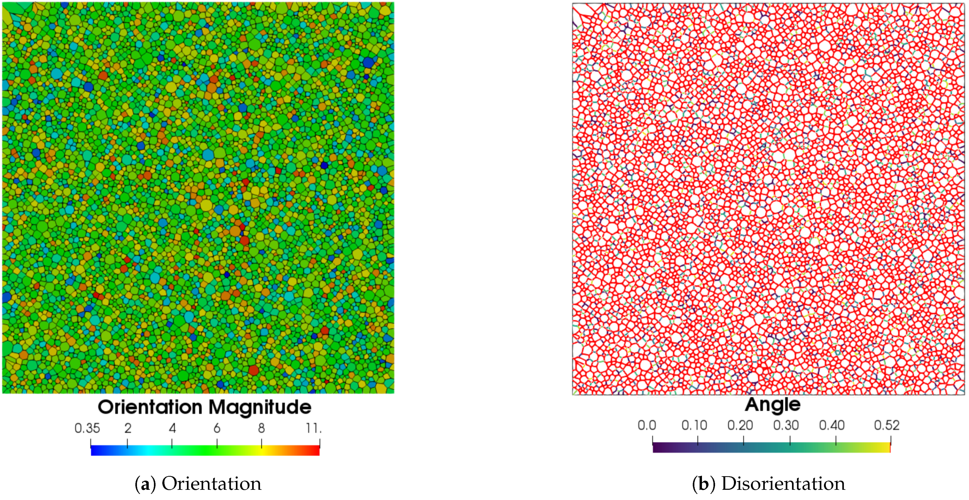
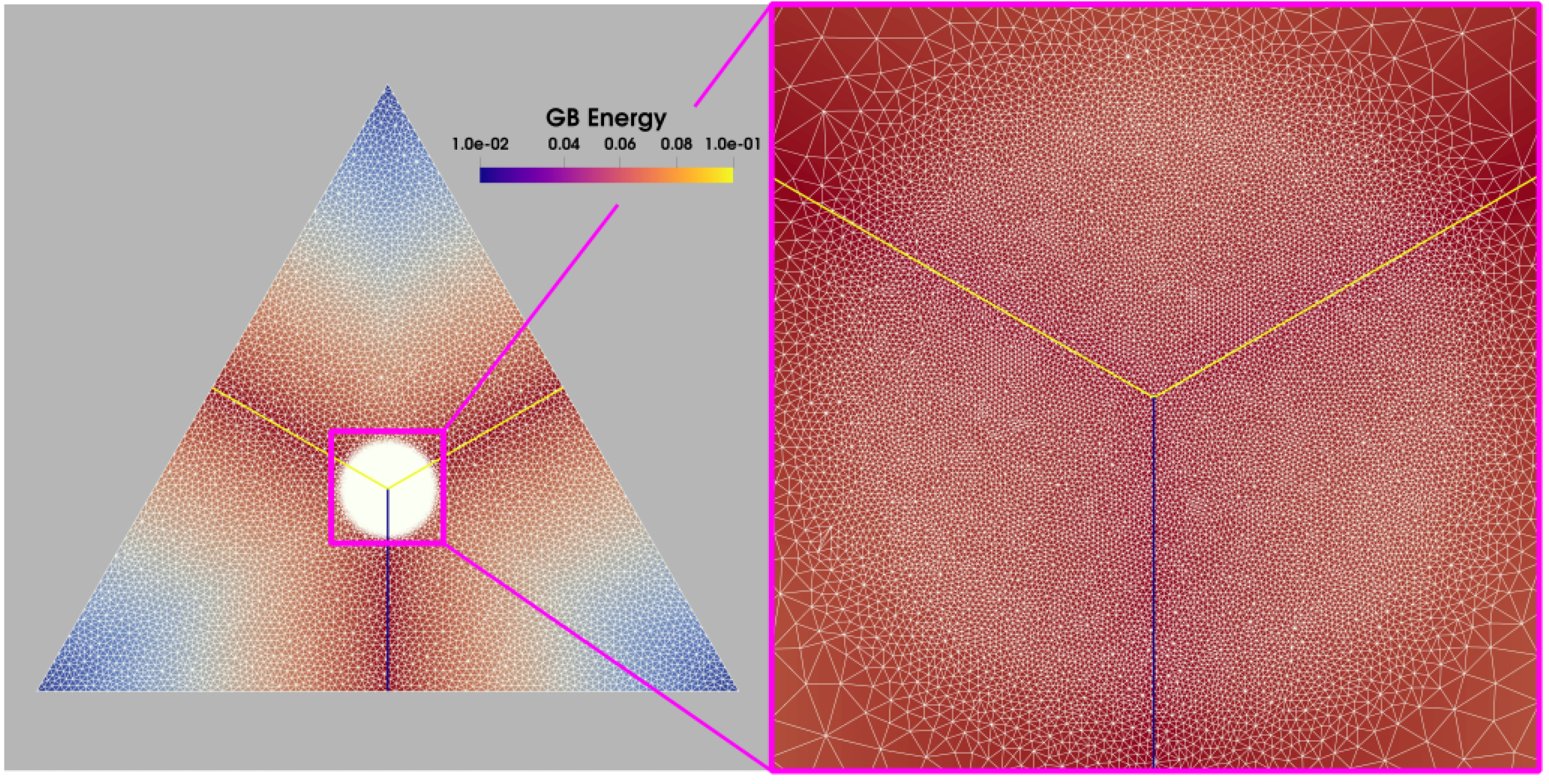
2.1. Crystallographic Definitions

Let us consider a domain ${\displaystyle \Omega }$ of dimension ${\displaystyle d}$ filled by ${\displaystyle n}$ grains ${\displaystyle G_i\in \Omega }$, being open spaces of ${\displaystyle \Omega }$ and defining the set of grains ${\displaystyle \mathcal{G}=\{G_i,i=1,\cdots ,N_G\}}$. The interface between two neighboring grains ${\displaystyle G_i}$ and ${\displaystyle G_j}$ constitutes a GB ${\displaystyle B_{ij}}$, and the whole set of boundaries form the GB network ${\displaystyle \Gamma }$. A boundary ${\displaystyle B_{ij}}$ is characterized by its morphology and its crystallographic properties, which are described using five variables: ${\displaystyle 2}$ shape properties, describing the interfaces by the unitary-outward normal direction ${\displaystyle n_{ij}}$, and ${\displaystyle 3}$ crystallographic properties describing the orientation relationship between the two adjacent grains, ${\displaystyle O_i}$ and ${\displaystyle O_j}$, known as the mis-orientation ${\displaystyle M_{ij}}$. As such, at the mesoscopic scale, each boundary may be characterized by a tuple:

$$\begin{array}{c}\hfill B_{ij}=(M_{ij},n_{ij}).\end{array}$$

The GB space, ${\displaystyle \mathcal{B}}$, parameterized by the mis-orientation and the normal direction is illustrated in Figure 1. The two quantities of interest, the GB energy ${\displaystyle \gamma }$ and the mobility ${\displaystyle \mu }$, are mapped from ${\displaystyle \mathcal{B}}$ to ${\displaystyle {\mathbb{R}}^{+}}$.

2.2. FE-LS Formulation

The LS method is a powerful tool firstly proposed by Osher and Sethian [40] to describe curvature flow of interfaces, enhanced later for evolving multiple junctions [41,42], and considered in recrystallization and grain growth problems in [17,36]. The principle for modeling polycrystals is as follows: the grain interfaces are defined through scalar fields called LS functions ${\displaystyle \varphi }$ in the space ${\displaystyle \Omega }$, and more precisely by the zero-isovalue of the ${\displaystyle \varphi }$ functions. LS functions to the interfaces are classically initialized as the sign Euclidean distance functions to these interfaces:

$$\begin{array}{c}\hfill \left\{\begin{array}{c}\varphi \left(X\right)=\pm d(X,\Gamma ),X\in \Omega ,\Gamma =\partial G\hfill \\ \varphi (X\in \Omega )=0\rightleftharpoons X\in \Gamma .\hfill \end{array}\right.\end{array}$$

(1)

with ${\displaystyle d}$ representing the Euclidean distance and ${\displaystyle \varphi }$ generally being defined as positive inside the grain and negative outside. The dynamics of the interface is studied by following the evolution of the LS field. The interface may be subjected to an arbitrary velocity field, ${\displaystyle \overrightarrow{v}}$, and its movement is described by solving the transport equation:

$$\begin{array}{c}\hfill {\displaystyle \frac{\partial \varphi }{\partial t}}+\overrightarrow{v}·\overrightarrow{\nabla }\varphi =0.\end{array}$$

(2)

The flexibility of this method lies in the ability to define different physical phenomena encapsulated in the velocity field. This equation is solved to describe the movement of every grain. When the number of grains increases, one may use a graph coloring/recoloring strategy [38] in order to drastically limit the number of involved LS functions: ${\displaystyle \Phi =\{{\varphi }_i,i=1,\cdots ,N\}}$, with ${\displaystyle N\ll N_G}$ being ${\displaystyle N_G}$, the number of grains. Additionally, two more treatments are necessary. Firstly, the LS functions are reinitialized at each time step to keep the metric property of a distance function:

$$\begin{array}{c}\hfill \parallel \nabla \varphi \parallel =1.\end{array}$$

(3)

Secondly, the evolution may not preserve the impenetrability constraints of the LS functions, leading to overlaps and voids between grain interfaces. These events are corrected after solving the transport equation by resolving Equation (4), as proposed in [41] and classically used in the LS framework [17,43]:

$$\begin{array}{c}\hfill {\varphi }_i\left(X\right)={\displaystyle \frac{1}{2}}\left[{\varphi }_i\left(X\right)-\underset{j\ne i}{max}{\varphi }_j\left(X\right)\right],\forall i=\{1,\cdots ,N\}.\end{array}$$

(4)

Several formulations using the LS framework exist in the literature. The initial GG formulation uses a homogeneous grain boundary energy and mobility, i.e., ${\displaystyle \gamma (\cancel{M},\cancel{n})}$ and ${\displaystyle \mu (\cancel{M},\cancel{n})}$ [17], and the velocity field is thus defined as:

$$\begin{array}{c}\hfill \overrightarrow{v}=\mu P\overrightarrow{n}=-\mu \gamma \kappa \overrightarrow{n},\end{array}$$

(5)

where ${\displaystyle P=-\gamma \kappa }$ is the capillarity pressure and ${\displaystyle n}$ is the outward unitary normal to the interface. When dealing with recrystallization, supplemental terms could be added to the velocity, as proposed in [17]. If ${\displaystyle \varphi }$ is defined as positive inside the grain and remains a distance function, the mean curvature and the normal may be defined as:

$$\begin{array}{c}\hfill \kappa =-\Delta \varphi ,\overrightarrow{n}=-\overrightarrow{\nabla }\varphi ,\end{array}$$

(6)

then, the velocity in Equation (5) may also be defined as:

$$\begin{array}{c}\hfill \overrightarrow{v}=-\mu \gamma \Delta \varphi \overrightarrow{\nabla }\varphi .\end{array}$$

(7)

Four different formulations will be studied. In the first one, an isotropic formulation is considered by introducing Equation (7) into Equation (2), thus the isotropic transport equation may be defined as a pure diffusive problem:

$$\begin{array}{c}\hfill {\displaystyle \frac{\partial \varphi }{\partial t}}-\mu \gamma \Delta \varphi =0.\end{array}$$

(8)

This formulation has shown good agreement with experimental data regarding GG predictions concerning the mean grain size and even the grain size distribution (GSD). However, this approach is limited when it comes to reproducing complex grain morphology (non-equiaxed ones), described as special grain boundaries, and with respect to textures. This formulation could be slightly modified in a second one with the introduction of heterogeneous GB properties, leading to a heterogeneous formulation:

$$\begin{array}{c}\hfill {\displaystyle \frac{\partial \varphi }{\partial t}}-\mu \left(M\right)\gamma \left(M\right)\Delta \varphi =0.\end{array}$$

(9)

With this formulation, it is expected to obtain more physical grain shapes. Indeed, some GBs can evolve faster thanks to higher grain boundary mobility values, and triple junctions may have different dihedral angles thanks to different GB energy values. This strategy, classically used in full-field formulations (not only in LS ones), can lead to confusion when it is named as “heterogeneous”. Indeed, stricto sensu, the heterogeneity shape of ${\displaystyle \mu }$ and ${\displaystyle \gamma }$ can lead to additional terms in the driving pressure of the kinetic equation, Equation (5), but also in the weak formulation derived to solve the GB motion. However, the term “heterogeneous” will be used in the following to distinguish this formulation from the purely isotropic model.

Such discussion is described in [26], where an additional term capturing the local heterogeneity of the multiple junctions is added to the velocity equation, such that:

$$\begin{array}{c}\hfill \overrightarrow{v}=\mu (\overrightarrow{\nabla }\gamma ·\overrightarrow{\nabla }\varphi -\gamma \Delta \varphi )\overrightarrow{\nabla }\varphi .\end{array}$$

(10)

Inserting this term into the transport equation, Equation (2), leads to the, hereafter called, “Heterogeneous with Gradient” formulation [26]:

$$\begin{array}{c}\hfill {\displaystyle \frac{\partial \varphi }{\partial t}}+\mu \overrightarrow{\nabla }\gamma ·\overrightarrow{\nabla }\varphi -\mu \gamma \Delta \varphi =0.\end{array}$$

(11)

The introduction of the term ${\displaystyle \overrightarrow{\nabla }\gamma ·\overrightarrow{n}}$ only acts at multiple junctions because these are the only places where this term does not vanish. This formulation is equivalent to the isotropic one if no heterogeneity is added.

Finally, in [33,44], a new relation for the velocity was developed using thermodynamics and differential geometry. The five crystalline parameters are taken into account with an intrinsic torque term, which leads to (see Equation (2.43) in [44]):

$$\begin{array}{c}\hfill {\displaystyle \frac{\partial \varphi }{\partial t}}-\mu \left({\displaystyle \frac{{\partial }^2\gamma }{\partial {\tilde{\nabla }}_{\alpha }\varphi \partial {\tilde{\nabla }}_{\beta }\varphi }}+\gamma m^{\alpha \beta }\right){\tilde{\nabla }}_{\alpha }{\tilde{\nabla }}_{\beta }\varphi +\mu P^{\alpha \beta }{\tilde{\nabla }}_{\beta }\gamma {\tilde{\nabla }}_{\alpha }\varphi =0,\end{array}$$

(12)

where ${\displaystyle m^{\alpha \beta }}$ is the metric with components ${\displaystyle \alpha }$ and ${\displaystyle \beta }$ of a Riemannian n-manifold, with ${\displaystyle n}$ the dimension of the space, and ${\displaystyle \tilde{\nabla }}$ the Levi-Civita connection. This equation may be redefined using a flat metric and tensor notations as:

$$\begin{array}{c}\hfill {\displaystyle \frac{\partial \varphi }{\partial t}}-\mu \left({\displaystyle \frac{{\partial }^2\gamma }{\partial \overrightarrow{n}\partial \overrightarrow{n}}}+\gamma \mathbb{I}\right):\mathbb{K}+\mu \mathbb{P}\overrightarrow{\nabla }\gamma ·\overrightarrow{\nabla }\varphi =0,\end{array}$$

(13)

and also written as:

$$\begin{array}{c}\hfill {\displaystyle \frac{\partial \varphi }{\partial t}}-\mu \left({\overrightarrow{\nabla }}_{\overrightarrow{n}}{\overrightarrow{\nabla }}_{\overrightarrow{n}}\gamma +\gamma \mathbb{I}\right):\mathbb{K}+\mu {\overrightarrow{\nabla }}_{\overrightarrow{n}}\gamma ·\overrightarrow{\nabla }\varphi =0,\end{array}$$

(14)

where ${\displaystyle \mathbb{I}}$ is the unitary matrix, ${\displaystyle \mathbb{P}=Id-\overrightarrow{n}\otimes \overrightarrow{n}}$ is the tangential projection tensor, and therefore, ${\displaystyle {\overrightarrow{\nabla }}_{\overrightarrow{n}}\gamma =\mathbb{P}\overrightarrow{\nabla }\gamma }$ with ${\displaystyle {\overrightarrow{\nabla }}_{\overrightarrow{n}}}$, the surface gradient on the unit sphere of interface normal ${\displaystyle \overrightarrow{n}}$, ${\displaystyle \mathbb{K}=\overrightarrow{\nabla }\overrightarrow{n}=\overrightarrow{\nabla }\overrightarrow{\nabla }\varphi }$, is the curvature tensor. In Equation (12), the term ${\displaystyle P^{\alpha \beta }{\tilde{\nabla }}_{\beta }\gamma {\tilde{\nabla }}_{\alpha }\varphi }$ and its equivalent ${\displaystyle \mathbb{P}\overrightarrow{\nabla }\gamma ·\overrightarrow{\nabla }\varphi }$ in Equation (13), i.e., ${\displaystyle {\overrightarrow{\nabla }}_n\gamma ·\overrightarrow{\nabla }\varphi }$, should be null in the grain interfaces. However, the front-capturing nature of the LS approach, which requires to solve Equation (13) not only at the GB network but also in its vicinity, needs to consider this term, which could be non-null around the GB interfaces. This stabilization term is then totally correlated to the front-capturing nature of the LS approach and not derived from the GG driving pressure. The resulting tensorial diffusion term, ${\displaystyle D={\overrightarrow{\nabla }}_{\overrightarrow{n}}{\overrightarrow{\nabla }}_{\overrightarrow{n}}\gamma +\gamma \mathbb{I}}$ [33,44], is also well-known as the GB stiffness tensor ${\displaystyle \Gamma \left(\overrightarrow{n}\right)}$ in [45,46]. With this formulation, the 5D-GB space ${\displaystyle \mathcal{B}}$ is fully described and is referred to as “Anisotropic-5”. If the torque term is neglected, the formulation used could be simplified as:

$$\begin{array}{c}\hfill {\displaystyle \frac{\partial \varphi }{\partial t}}+\mu \mathbb{P}\overrightarrow{\nabla }\gamma ·\overrightarrow{\nabla }\varphi -\mu \gamma \Delta \varphi =0.\end{array}$$

(15)

This equation is hereafter called “Anisotropic” and is not equivalent to the “Heterogeneous with Gradient” formulation Equation (11). The strong formulations used in this work are finally the ones defined by the Equations (8), (9), (11) and (15). Moreover, the effect of heterogeneous GB mobility is take into account in the weak formulations in the form of a GB mobility gradient in the Heterogeneous with Gradient and Anisotropic formulations. The weak formulations of Equations (8), (9), (11) and (15), with ${\displaystyle \phi \in H_0^1(\Omega )}$, can be summarized as:

$$\begin{array}{c}\hfill {\int }_{\Omega }{\displaystyle \frac{\partial \varphi }{\partial t}}\phi d\Omega +{\int }_{\Omega }\mu \gamma \overrightarrow{\nabla }\phi ·\overrightarrow{\nabla }\varphi d\Omega -{\int }_{\partial \Omega }\mu \gamma \phi \overrightarrow{\nabla }\varphi ·\overrightarrow{n}d(\partial \Omega )=0,\end{array}$$

(16)

$$\begin{array}{c}\hfill {\int }_{\Omega }{\displaystyle \frac{\partial \varphi }{\partial t}}\phi d\Omega +{\int }_{\Omega }\mu \left(M\right)\gamma \left(M\right)\overrightarrow{\nabla }\phi ·\overrightarrow{\nabla }\varphi d\Omega -{\int }_{\partial \Omega }\mu \left(M\right)\gamma \left(M\right)\phi \overrightarrow{\nabla }\varphi ·\overrightarrow{n}d(\partial \Omega )=0,\end{array}$$

(17)

$$\begin{array}{c}\hfill \begin{array}{c}\hfill {\int }_{\Omega }{\displaystyle \frac{\partial \varphi }{\partial t}}\phi d\Omega +{\int }_{\Omega }\mu \gamma \overrightarrow{\nabla }\phi ·\overrightarrow{\nabla }\varphi d\Omega -{\int }_{\partial \Omega }\mu \gamma \phi \overrightarrow{\nabla }\varphi ·\overrightarrow{n}d(\partial \Omega )+\\ \hfill +2{\int }_{\Omega }\mu \overrightarrow{\nabla }\gamma ·\overrightarrow{\nabla }\varphi \phi d\Omega +{\int }_{\Omega }\gamma \overrightarrow{\nabla }\mu ·\overrightarrow{\nabla }\varphi \phi d\Omega =0,\end{array}\end{array}$$

(18)

and

$$\begin{array}{c}\hfill \begin{array}{c}\hfill {\int }_{\Omega }{\displaystyle \frac{\partial \varphi }{\partial t}}\phi d\Omega +{\int }_{\Omega }\mu \gamma \overrightarrow{\nabla }\phi ·\overrightarrow{\nabla }\varphi d\Omega -{\int }_{\partial \Omega }\mu \gamma \phi \overrightarrow{\nabla }\varphi ·\overrightarrow{n}d(\partial \Omega )+\\ \hfill {\int }_{\Omega }\mu (\mathbb{P}·\overrightarrow{\nabla }\gamma +\overrightarrow{\nabla }\gamma )\phi \overrightarrow{\nabla }\varphi d\Omega +{\int }_{\Omega }\gamma \overrightarrow{\nabla }\mu ·\overrightarrow{\nabla }\varphi \phi d\Omega =0,\end{array}\end{array}$$

(19)

All the presented formulations are equivalent if the properties are homogeneous, but the main question remains as to the test of their capacity otherwise. In the next sections, a comparative study is presented. In the following, the “Isotropic”, “Heterogeneous”, “Heterogeneous with Gradient”, and “Anisotropic” formulations will be referred to as Iso, Het, HetGrad, and Aniso. It must be highlighted that the formulations proposed in Equations (18) and (19) are slightly more general than those proposed in [26,33] respectively, as here, ${\displaystyle \mu }$ is also considered as heterogeneous.

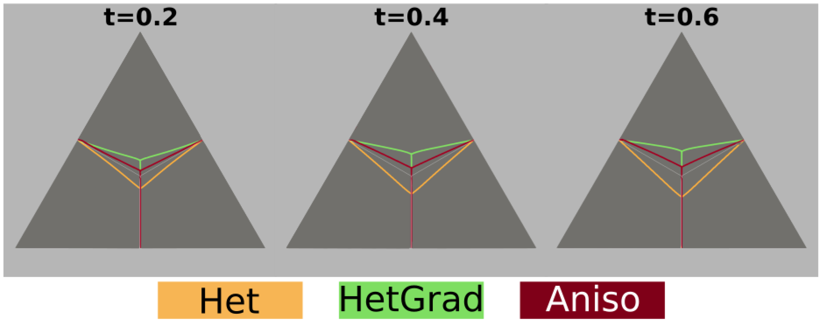
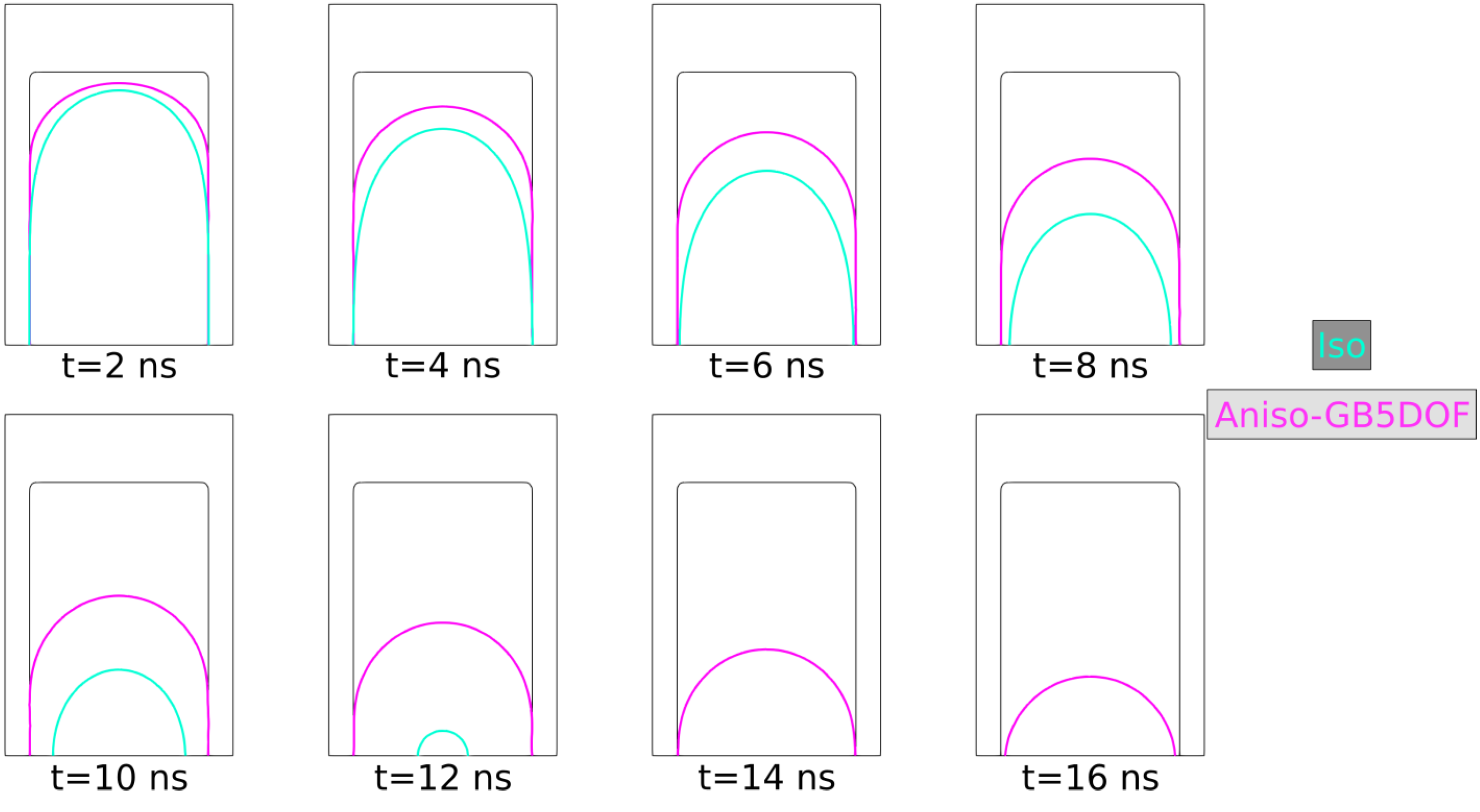
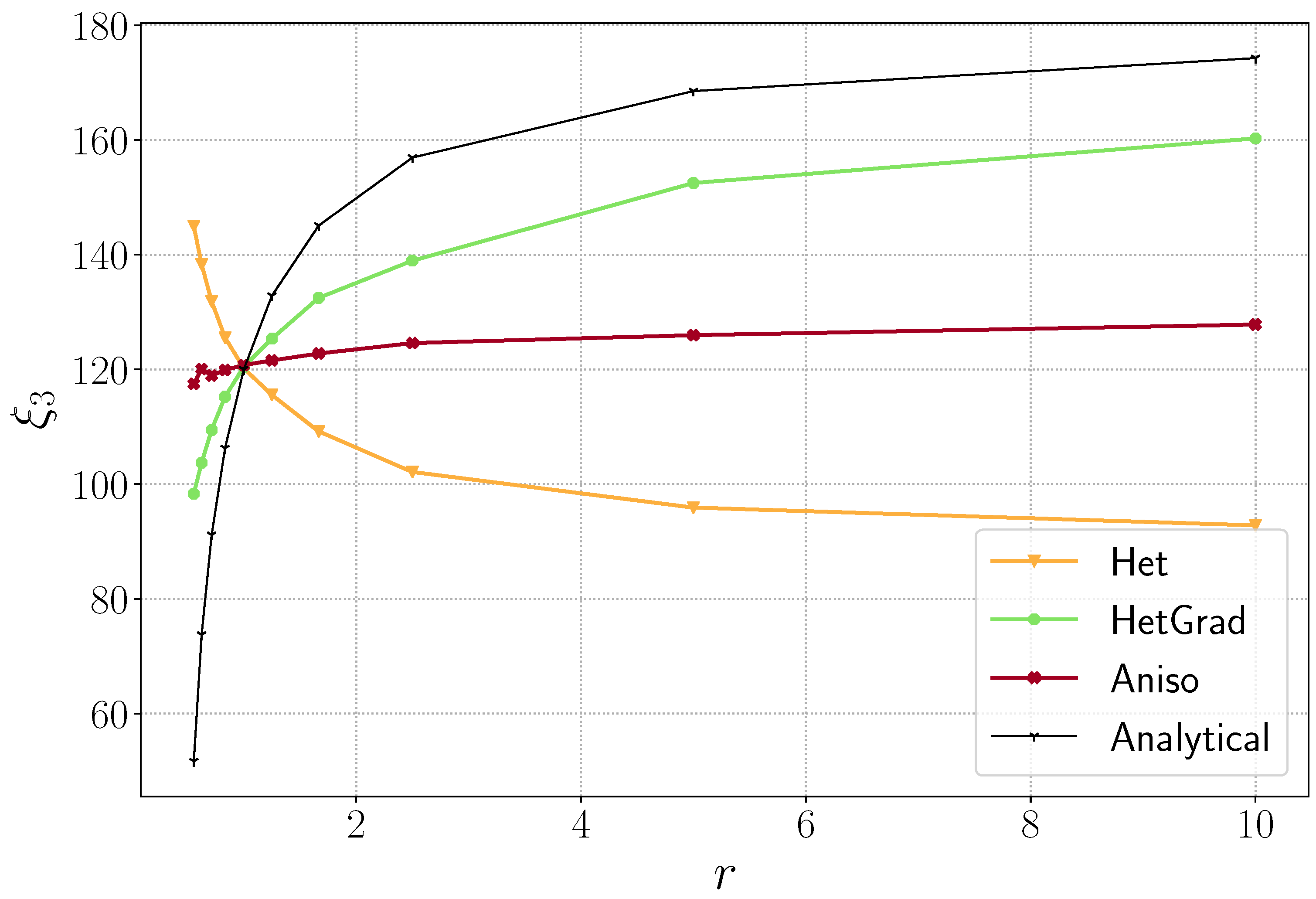
3. The Grim Reaper Case

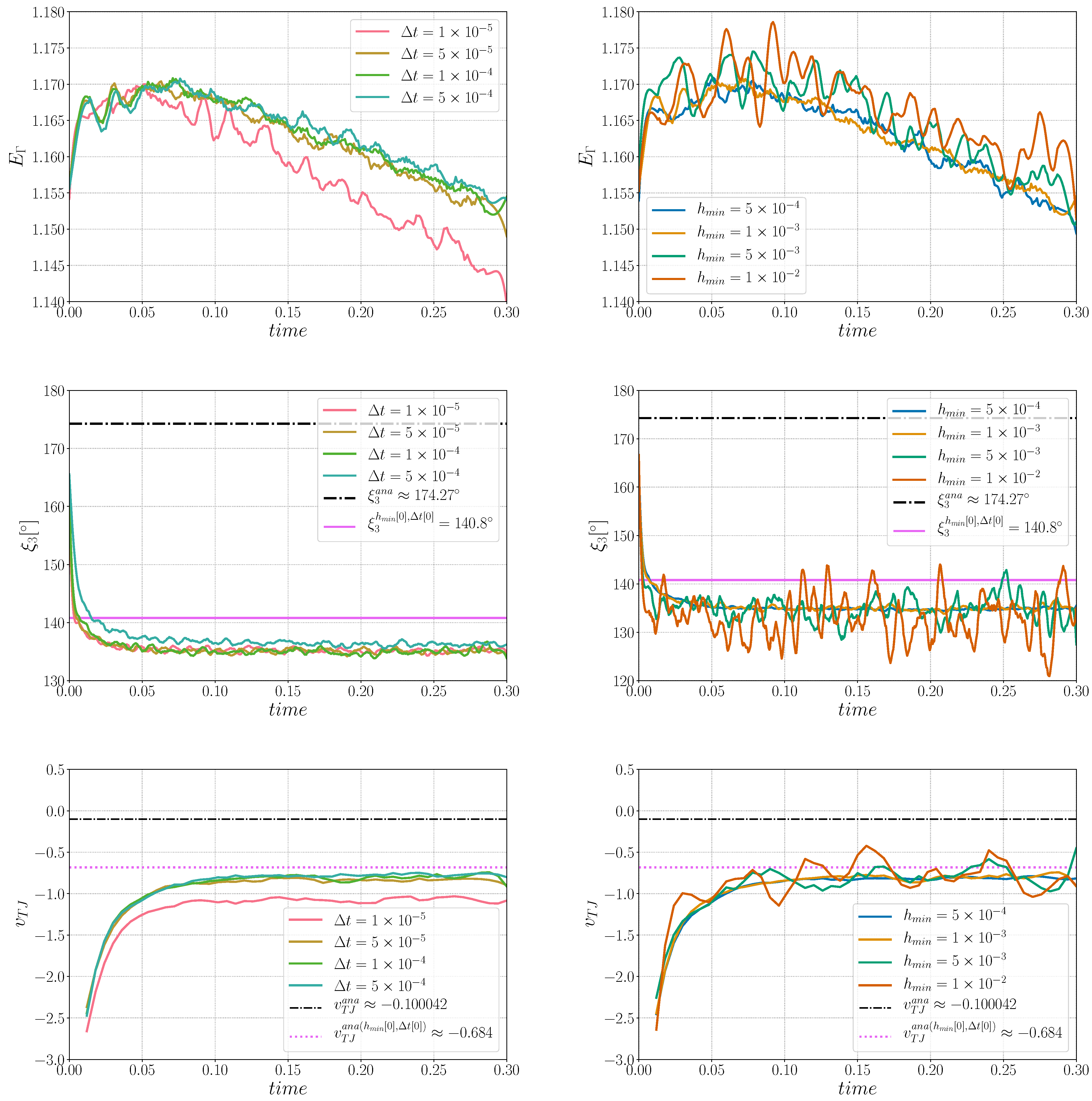
3.1. Description of the Test Case

In this section, simulation results obtained with the Het, HetGrad, and Aniso formulations are compared for a 2D-triple junction configuration proposed in [6] and described in Figure 2. The initial microstructure is a dimensionless T-shape triple junction with ${\displaystyle L_x=1}$ and ${\displaystyle L_y=3}$. This geometry was chosen because after a transient-state, a quasi-steady-state is reached, where analytical relations, depending on the reduced mobility, are available for the triple junction velocity and equilibrium angles.

When the quasi-steady-state is reached, the triple junction moves with a constant velocity towards the bottom of the domain, with a stable triple junction profile which respects the conditions imposed by the Herring’s equation [47]:

$$\sum _{j>i}{\gamma }_{ij}{\overrightarrow{\tau }}_{ij}+{\displaystyle \frac{\partial {\gamma }_{ij}}{\partial {\overrightarrow{\tau }}_{ij}}}=0,$$

(20)

where ${\displaystyle {\gamma }_{ij}}$ is the GB energy and ${\displaystyle {\overrightarrow{\tau }}_{ij}}$ are the inward pointing tangent vectors of the three boundaries at the triple junction. In the present example, the grain boundary energy is constant per interface (${\displaystyle \gamma \left(M\right)}$) and the above equation may as well be expressed by the Young’s law (no torque terms):

$$\sum _{j>i}{\gamma }_{ij}{\overrightarrow{\tau }}_{ij}=0,$$

(21)

which may be expressed in terms of the angles ${\displaystyle {\xi }_i}$ of the grain ${\displaystyle i}$, through the Young’s equilibrium (see Figure 2):

$${\displaystyle \frac{sin{\xi }_1}{{\gamma }_{23}}}={\displaystyle \frac{sin{\xi }_2}{{\gamma }_{13}}}={\displaystyle \frac{sin{\xi }_3}{{\gamma }_{12}}}.$$

(22)

By considering an axially symmetric configuration where ${\displaystyle {\gamma }_{13}={\gamma }_{23}={\gamma }_{top}}$ and ${\displaystyle {\gamma }_{12}={\gamma }_{bot}}$, and by defining the ratio of grain boundary energies as ${\displaystyle r=\frac{{\gamma }_{top}}{{\gamma }_{bot}}}$, an analytical value for the angle ${\displaystyle {\xi }_3}$ can be obtained:

$${\xi }_3^{ana}=2arccos\left({\displaystyle \frac{1}{2r}}\right).$$

(23)

Moreover, the stationary transported profile takes the form of the “Grim Reaper” profile, defined as:

$$\left\{\begin{array}{c}y(x,t)=g\left(x\right)+v_{TJ}^{ana}t\hfill \\ g\left(x\right)=-{\displaystyle \frac{\mu {\gamma }_{top}}{v_{TJ}^{ana}}}ln\left(cos\left({\displaystyle \frac{v_{TJ}^{ana}}{\mu {\gamma }_{top}}}x\right)\right)+y_0\hfill \end{array}\right.$$

(24)

where ${\displaystyle v_{TJ}^{ana}}$ is the magnitude of the stationary velocity, ${\displaystyle y_0}$ is the initial y-value, and ${\displaystyle (x,y)}$ are the Cartesian coordinates. By using Neumann boundary conditions, the stationary velocity could be related to the x-size of the domain:

$$v_{TJ}^{ana}=-{\displaystyle \frac{2\mu {\gamma }_{top}}{L_x}}\left({\displaystyle \frac{\pi }{2}}-{\displaystyle \frac{{\xi }_3^{ana}}{2}}\right).$$

(25)

In order to focus on a considerable level of heterogeneity in the system, ${\displaystyle r}$ is initially fixed as equal to 10 (${\displaystyle {\gamma }_{top}=1}$ and ${\displaystyle {\gamma }_{bot}=0.1}$), and ${\displaystyle \mu }$ is defined as unitary. Several simulations were carried out and compared with the analytical values of ${\displaystyle {\xi }_3^{ana}=174.{27}^{\circ }}$ and ${\displaystyle v_{TJ}^{ana}=-0.100042}$. These variables are computed as follows:

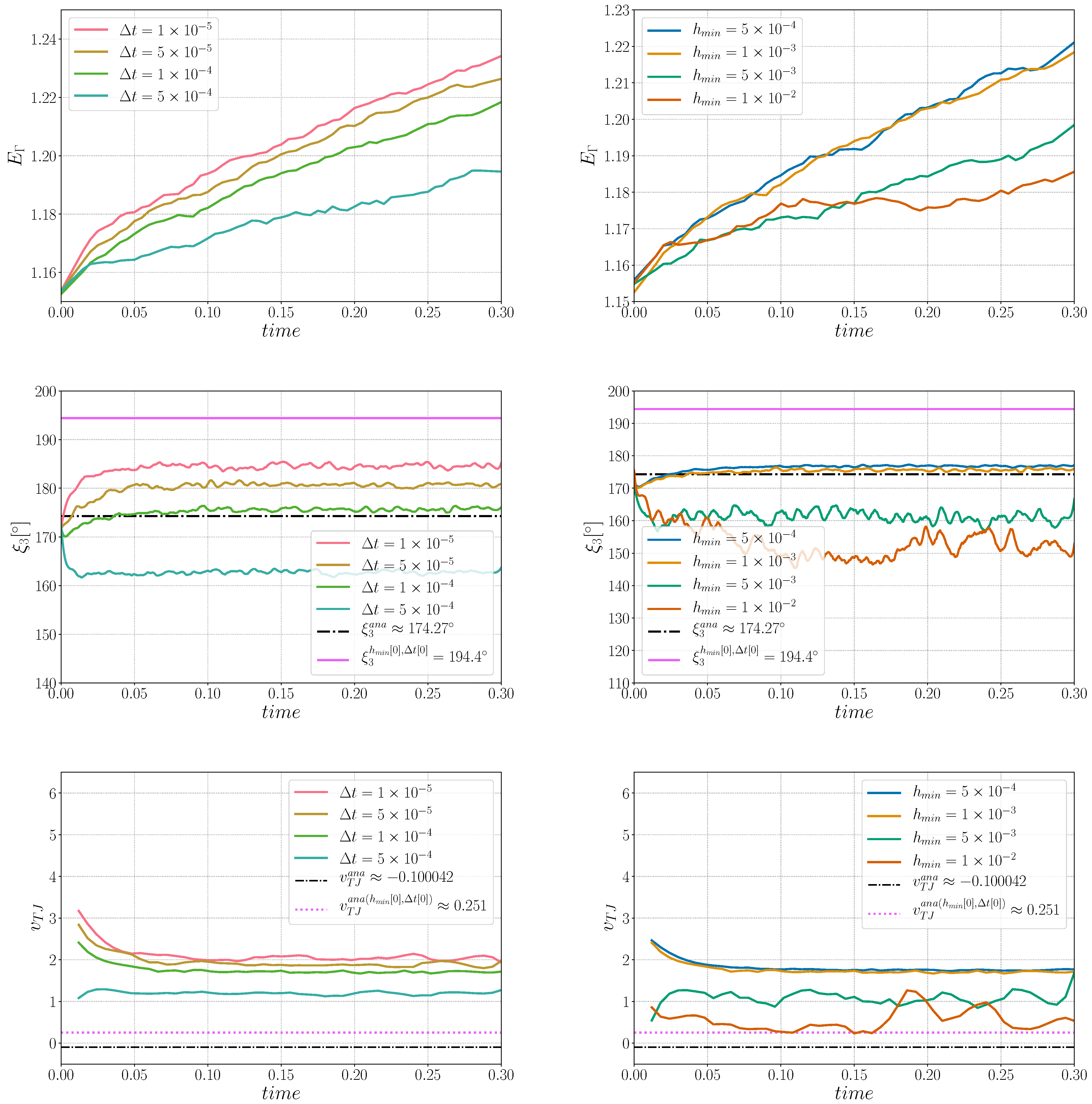
• The velocity of the triple junction is computed using the relation ${\displaystyle v_{TJ}=\left(y_{TJ}^{t+\Delta t}-y_{TJ}^t\right)/\Delta t}$, where ${\displaystyle y_{TJ}^t}$ is the y-position of the triple point at time ${\displaystyle t}$ and ${\displaystyle \Delta t}$ is the time step.
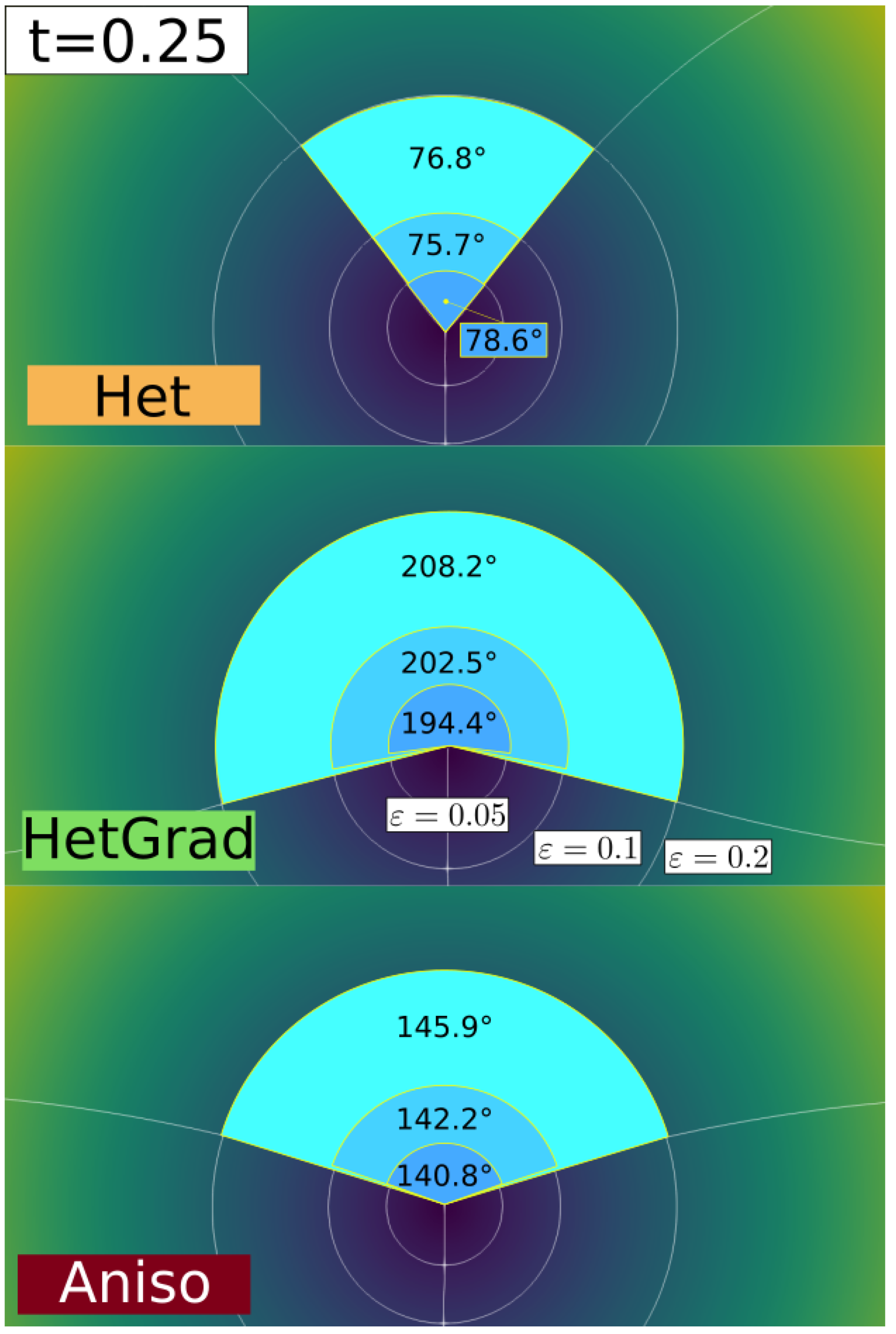
• The dihedral angles are computed using the methodology presented in [26]: one may define, at each time, a circle of radius ${\displaystyle \epsilon }$ with circumference ${\displaystyle {\mathcal{C}}_{\epsilon }}$, and divide it into arcs which pass through grain ${\displaystyle G_i}$ with length ${\displaystyle {\mathcal{L}}_{\epsilon }^i}$. The angle of the arc, ${\displaystyle {\xi }_i}$, could be approximated thanks to the relation ${\displaystyle {\xi }_i=2\pi {\mathcal{L}}_{\epsilon }^i/{\mathcal{C}}_{\epsilon }}$.

Hence, these variables are affected by the spatial discretization of the domain and the choice of ${\displaystyle \epsilon }$, which must be close enough to the multiple junction while containing a sufficient number of finite elements, as illustrated in Figure 3, where different values of ${\displaystyle ϵ}$ are tested. Here, the value ${\displaystyle \epsilon =0.05}$ is adopted. ${\displaystyle v_{TJ}}$ and ${\displaystyle {\xi }_i}$ are compared using relative errors which are defined as:

$$e_X=\left|{\displaystyle \frac{X^{ana}-X}{X^{ana}}}\right|,$$

where ${\displaystyle X^{ana}}$ is the analytical value of the variable to be compared. Another discussed quantity is the interfacial energy, calculated using:

$$E_{\Gamma }=\sum _i\sum _{e\in \mathcal{T}}{\displaystyle \frac{1}{2}}\gamma l_e\left({\varphi }_i\right),$$

(26)

where ${\displaystyle \mathcal{T}}$ is the set of all elements in the FE mesh, ${\displaystyle l_e}$ is the length of the zero iso-value existing in the element ${\displaystyle e}$, and ${\displaystyle i}$ refers to the number of LS functions, and the ${\displaystyle {\displaystyle \frac{1}{2}}}$ is necessary due to the duplicity of the LS functions in the interfaces defining a grain boundary. This variable is frequently studied and it may be seen as an energetic measure of how quickly the system reaches equilibrium.

3.2. Numerical Strategy

The simulations presented here were carried out with unstructured triangular meshes, a P1 interpolation, and using an implicit backward Euler time scheme for the time discretization. The system is assembled using typical P1 FE elements with a Streamline Upwind Petrov–Galerkin (SUPG) stabilization for the convective term [48]. The boundary conditions (BCs) are classical null-von Neumann BCs applied to all of the LS functions. This choice imposes the orthogonality between the LS functions and the boundary domain (each plane of the boundary domain can be seen as a symmetric plane). By considering a minimal and maximal mesh size (respectively ${\displaystyle h_{min}}$ and ${\displaystyle h_{max}}$), an optimized anisotropic re-meshing strategy developed by Bernacki et al. [37,49], used in the DIGIMU${\displaystyle {}^{\circledR }}$ software [50] and illustrated in Figure 4, is adopted here. The mesh is finely and anisotropically refined close to the interfaces (${\displaystyle \varphi <{\varphi }_{min}}$) and becomes isotropic when ${\displaystyle \varphi >{\varphi }_{max}}$, with a linear evolution of the normal mesh size between ${\displaystyle {\varphi }_{min}}$ and ${\displaystyle {\varphi }_{max}}$. A homogeneous tangential mesh size (${\displaystyle h_t=h_{max}}$) is considered everywhere and the normal mesh size is then defined as:

$$\left\{\begin{array}{c}{h}_n=h_{min},\varphi <{\varphi }_{min},\hfill \\ h_n=m(\varphi -{\varphi }_{min})+h_{min},m={\displaystyle \frac{h_{max}-h_{min}}{{\varphi }_{max}-{\varphi }_{min}}}{\varphi }_{min}\le \varphi \le {\varphi }_{max},\hfill \\ h_n=h_t=h_{max},\varphi >{\varphi }_{max}.\hfill \end{array}\right.$$

(27)

By generalizing this approach at the multiple junctions, a fine isotropic (${\displaystyle h_n=h_t=h_{min}}$) re-meshing is automatically performed (see [37] for more details). During grain boundary migration, thanks to a topological mesher/re-mesher, anisotropic re-meshing operations are performed periodically to follow the grain interfaces. Typically, a re-meshing operation is considered each time a LS is about to leave the fine mesh area set by ${\displaystyle {\varphi }_{min}}$.

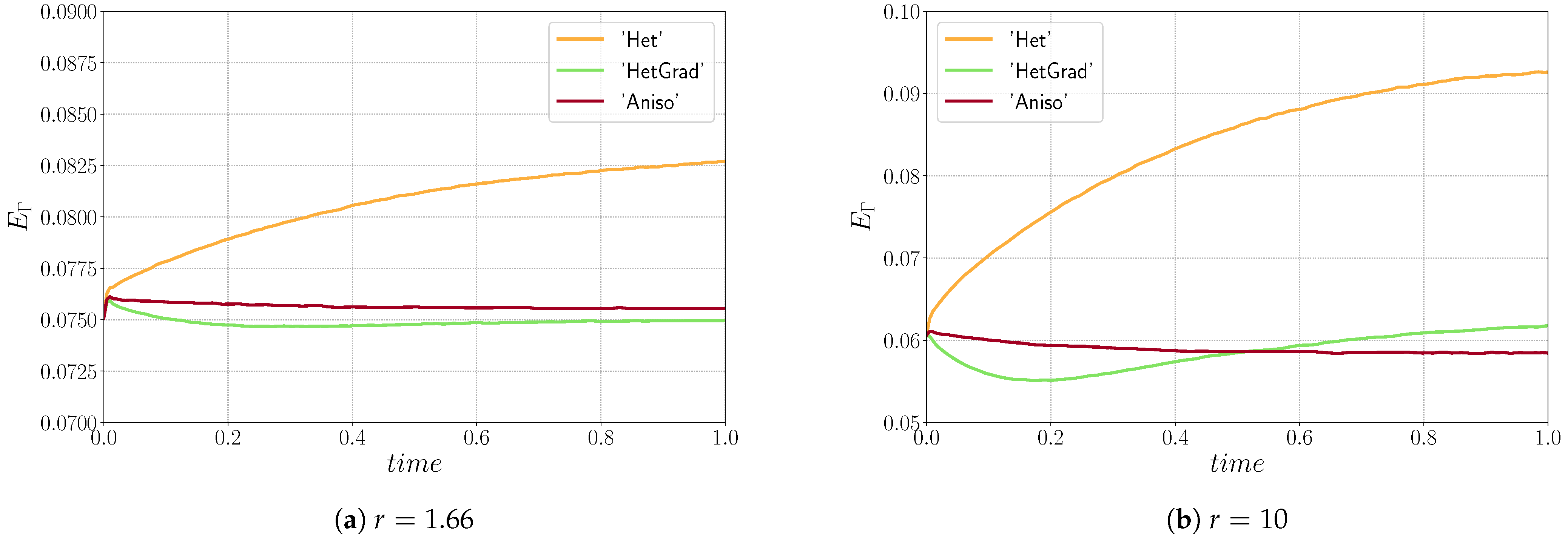
3.3. Results and Analysis

First, a sensibility analysis for the three formulations was carried out. The values of mesh size and time step used here are: ${\displaystyle h_{max}=h_t=1\times {10}^{-2}}$, ${\displaystyle h_{min}=\{5\times {10}^{-4},1\times {10}^{-3},5\times {10}^{-3},1\times {10}^{-2}\}}$ and ${\displaystyle \Delta t=\{1\times {10}^{-5},5\times {10}^{-5},1\times {10}^{-4},5\times {10}^{-4}\}}$. For all the cases, ${\displaystyle {\Phi }_{min}}$ and ${\displaystyle {\Phi }_{max}}$ are fixed respectively to ${\displaystyle 1\times {10}^{-2}}$ and ${\displaystyle 2\times {10}^{-2}}$. Figure 3 shows, for the different formulations, the triple junctions at ${\displaystyle t=0.25}$ using ${\displaystyle h_{min}=5\times {10}^{-4}}$ and ${\displaystyle \Delta t=1\times {10}^{-5}}$. One dihedral angle is depicted for different values of ${\displaystyle \epsilon }$. In the following, ${\displaystyle {\xi }_3^{h_{min}\left[k\right],\Delta t\left[k\right]}}$ is used to define the converged value of the ${\displaystyle {\xi }_3}$ angle for the ${\displaystyle k}$-th value of the ${\displaystyle h_{min}}$ and ${\displaystyle \Delta t}$ datasets. Indeed, if the results described in Figure 5, Figure 6 and Figure 7 principally aim to compare the simulations with the quasi-steady-state analytical values, it is also interesting to discuss the obtained converged value of ${\displaystyle v_{TJ}}$ as a function of the converged value of ${\displaystyle {\xi }_3}$ (i.e., if Equation (25) is respected for these values).

Figure 5 illustrates the evolution of ${\displaystyle E_{\Gamma }}$, ${\displaystyle {\xi }_3}$, and ${\displaystyle v_{TJ}}$ using the Het formulation. Two stages appear in ${\displaystyle E_{\Gamma }}$, whereby it initially increases before decreasing. The results illustrate the fact that the approach seems not to converge, in time and space, towards the analytical solutions. However, in terms of the dihedral angle, the results converge towards ${\displaystyle {\xi }_3^{h_{min}\left[0\right],\Delta t\left[0\right]}}$, and the triple junction velocity converges toward the corresponding velocity ${\displaystyle v_{TJ}^{ana(h_{min}\left[0\right],\Delta t\left[0\right])}}$ (following Equation (25)). The movement of the Het formulation is mostly influenced by the curvature of the interface, as exposed in Section 2, and one has to keep in mind that there are no additional terms that could influence the movement of the interfaces. These results illustrate that the Het formulation, by considering heterogenous values of reduced mobility and the multiple junction treatment defined by Equation (3), without re-discussing the capillarity driving pressure used in the kinetic equations, is definitively not a good option when a convective/diffusive formulation is solved to model the GG mechanism.

The evolution of the HetGrad formulation is quite different, the interface evolves in the opposite direction (see Figure 8) which explains that ${\displaystyle E_{\Gamma }}$ increases during the simulation (see Figure 6). An explanation of this evolution comes from the presence of the grain boundary energy gradient, ${\displaystyle \nabla \gamma }$, in the triple junction. The main purpose of this gradient is the correction of the triple junction dihedral angles and velocity. In Figure 6, one can see that ${\displaystyle {\xi }_3}$ is closer to its analytical value and it also converges towards ${\displaystyle {\xi }_3^{h_{min}\left[0\right],\Delta t\left[0\right]}}$. Nevertheless, ${\displaystyle \nabla \gamma }$ also changes the kinetics of the interface because it is present along the interface and exerts a force that overcomes the effect of the curvature and generates a movement in the opposite direction. Regarding the velocity, it does not converge towards the analytical value ${\displaystyle v_{TJ}^{ana}}$, nor the correlated value ${\displaystyle v_{TJ}^{ana(h_{min}\left[0\right],\Delta t\left[0\right])}}$.

The Aniso formulation has an additional term, the projection tensor ${\displaystyle \mathbb{P}}$, which takes into account the tangential changes of ${\displaystyle \nabla \gamma }$. Thanks to this term, the interface evolves in the right direction, with a minimization of the boundary energy. From the evolution of ${\displaystyle {\xi }_3}$ and ${\displaystyle v_{TJ}}$, one can see that the simulation converges in time and space. Even if the values of ${\displaystyle {\xi }_3}$ do not precisely fit the analytical value, they converge towards ${\displaystyle {\xi }_3^{h_{min}\left[0\right],\Delta t\left[0\right]}}$. Moreover, the converged value of velocity is around ${\displaystyle v_{TJ}^{ana(h_{min}\left[0\right],\Delta t\left[0\right])}}$, meaning that the kinetics and topology of the triple junction are well-correlated through Equation (25).

The evolution of the triple junction profile using the Het, HetGrad, and Aniso formulations is illustrated in Figure 8. Both the Het and Aniso formulations produced the Grim Reaper profile, while the profile produced by the HetGrad formulation evolves in the opposite direction. This is reflected in the values of the triple junction velocity shown in Figure 9c. From the comparison of the interfacial energy evolution (Figure 9a) and of the velocities (Figure 9c), one can see that the Aniso formulation has the best energetic behavior and a better approximation of the triple junction velocity. However, the best approximation of dihedral angles is obtained with the HetGrad formulation (Figure 9b).

The level of anisotropy defined here is high (${\displaystyle r=10}$), and this order of value has also been discussed in the literature [26,30,51] and remains necessary to discuss realistic polycrystal aggregates (coherent twin energy, for example). In Figure 10, the effect of the anisotropy level (${\displaystyle r}$ value) on the top dihedral angle and the triple junction velocity is illustrated. We have carried out simulations using ${\displaystyle h=1\times {10}^{-3}}$, ${\displaystyle \Delta t=1\times {10}^{-4}}$ and ${\displaystyle r\in \{0.55,0.625,0.714,0.833,1.0,1.25,1.66,2.5,5,10\}}$, which are equivalent to ${\displaystyle {\gamma }_{bot}\in \{1.8,1.6,1.4,1.2,1.0,0.8,0.6,0.4,0.2,0.1\}}$. These results allow us to conclude that the Het methodology is not adapted whatever the ${\displaystyle r}$ value. Interestingly, the HetGrad formulation seems very good for ${\displaystyle {\xi }_3}$ and ${\displaystyle v_{TJ}}$ for ${\displaystyle r<1.5}$, but the migration direction ends up being reversed for higher r values, while keeping an excellent profile for the equilibrium angles. Finally, if the angle respect is slightly worse for the Aniso formulation, the respect of the triple junction speed is much better as soon as ${\displaystyle r>1}$. In Figure 10b, the three additional dashed lines represent the expected velocity for the ${\displaystyle {\xi }_3}$ values obtained after reaching equilibrium, as illustrated in Figure 10a using Equation (25). One can see that the Het and HetGrad formulations correlate ${\displaystyle {\xi }_3}$ and ${\displaystyle v_{TJ}}$ for ${\displaystyle r<1}$. On the other hand, the Aniso formulation correlates ${\displaystyle {\xi }_3}$ and ${\displaystyle v_{TJ}}$ for every ${\displaystyle r}$ value. A good correlation could be advantageous if one wants to perform more realistic simulations where correct kinetics and topology of the microstructure are of significant importance. An additional analysis is presented in the Appendix A, where a modified Grim Reaper case with Dirichlet boundary conditions is detailed. The obtained results have similar trends to those presented in Figure 10a.

3.4. Conclusions

These results highlight that the Aniso formulation seems to be the most physically acceptable approach regarding the velocity of the triple junction and the interfacial energy evolution. Additionally, it also correctly represents the dihedral angles for a wide range of anisotropy levels. Nevertheless, these results must be reinforced with large-scale simulations of polycrystals, which is the subject of the next section.

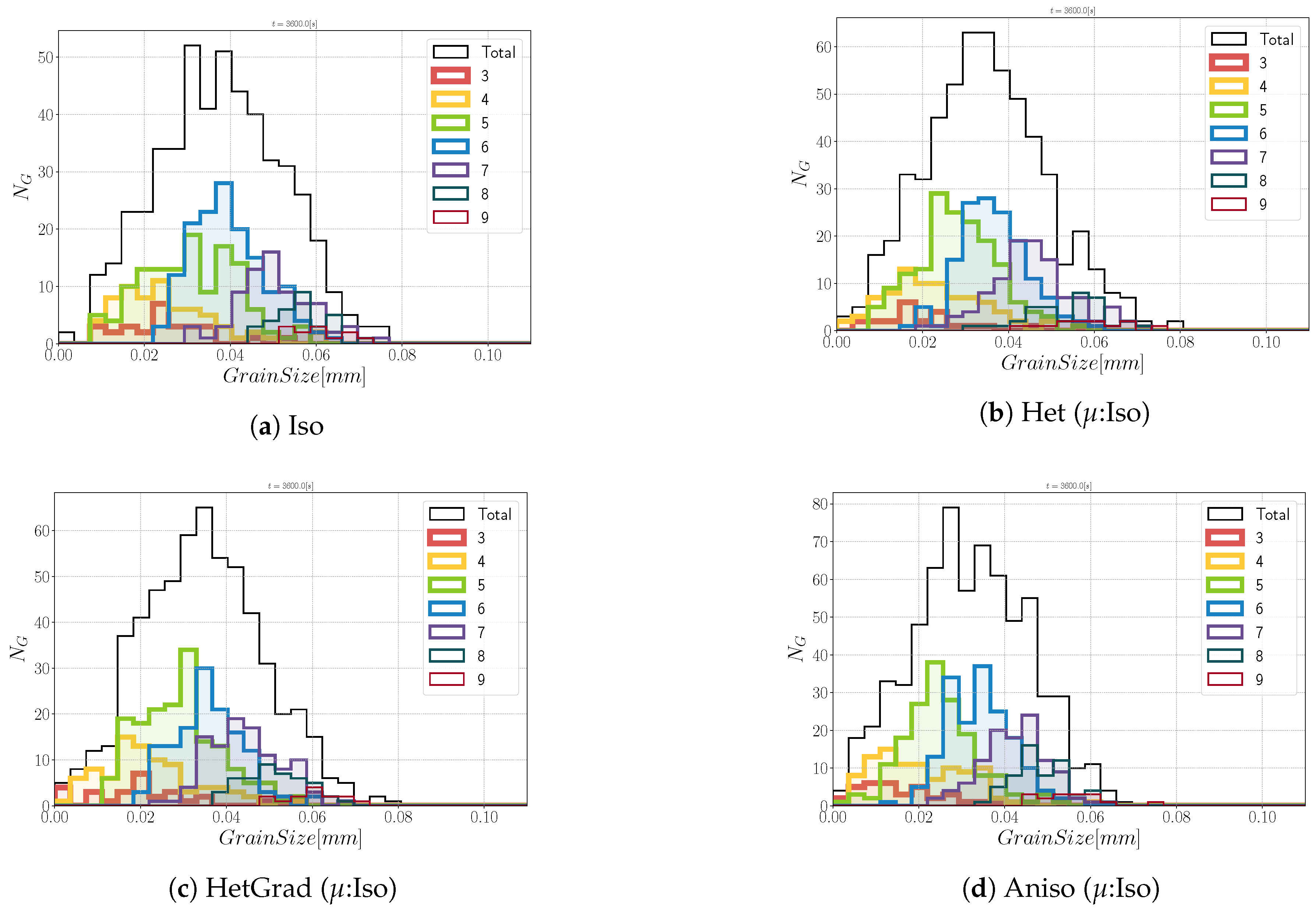
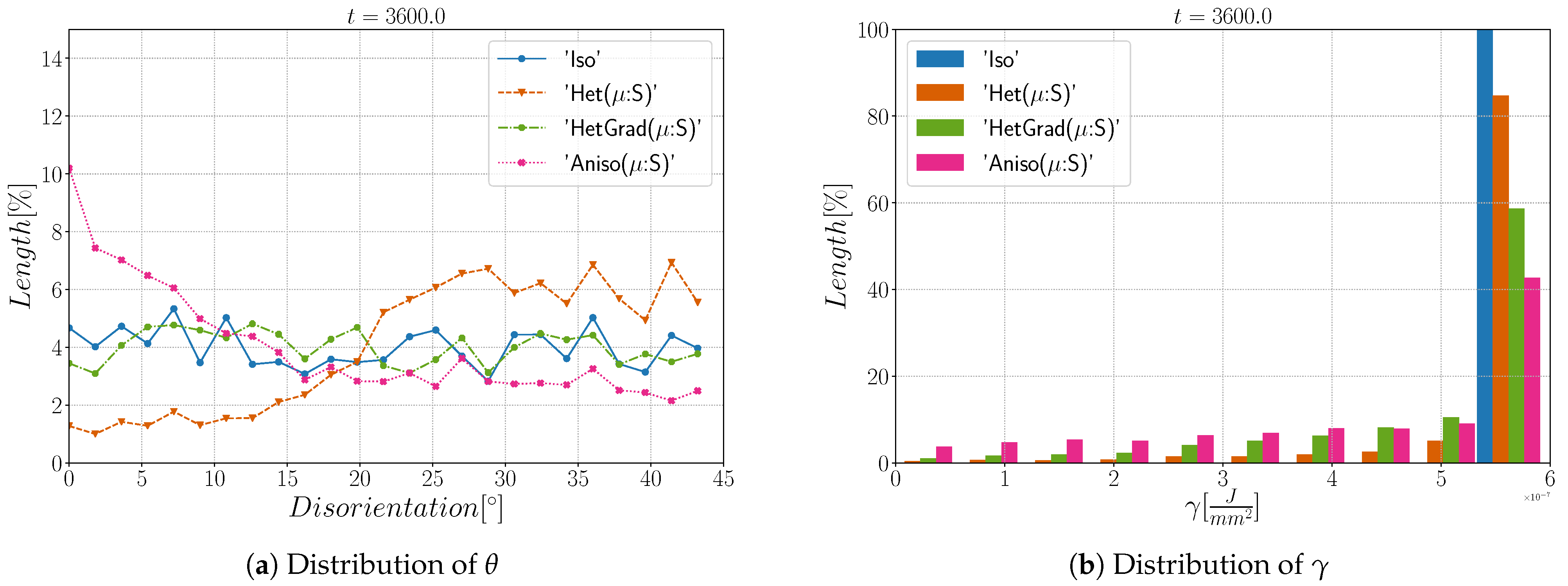
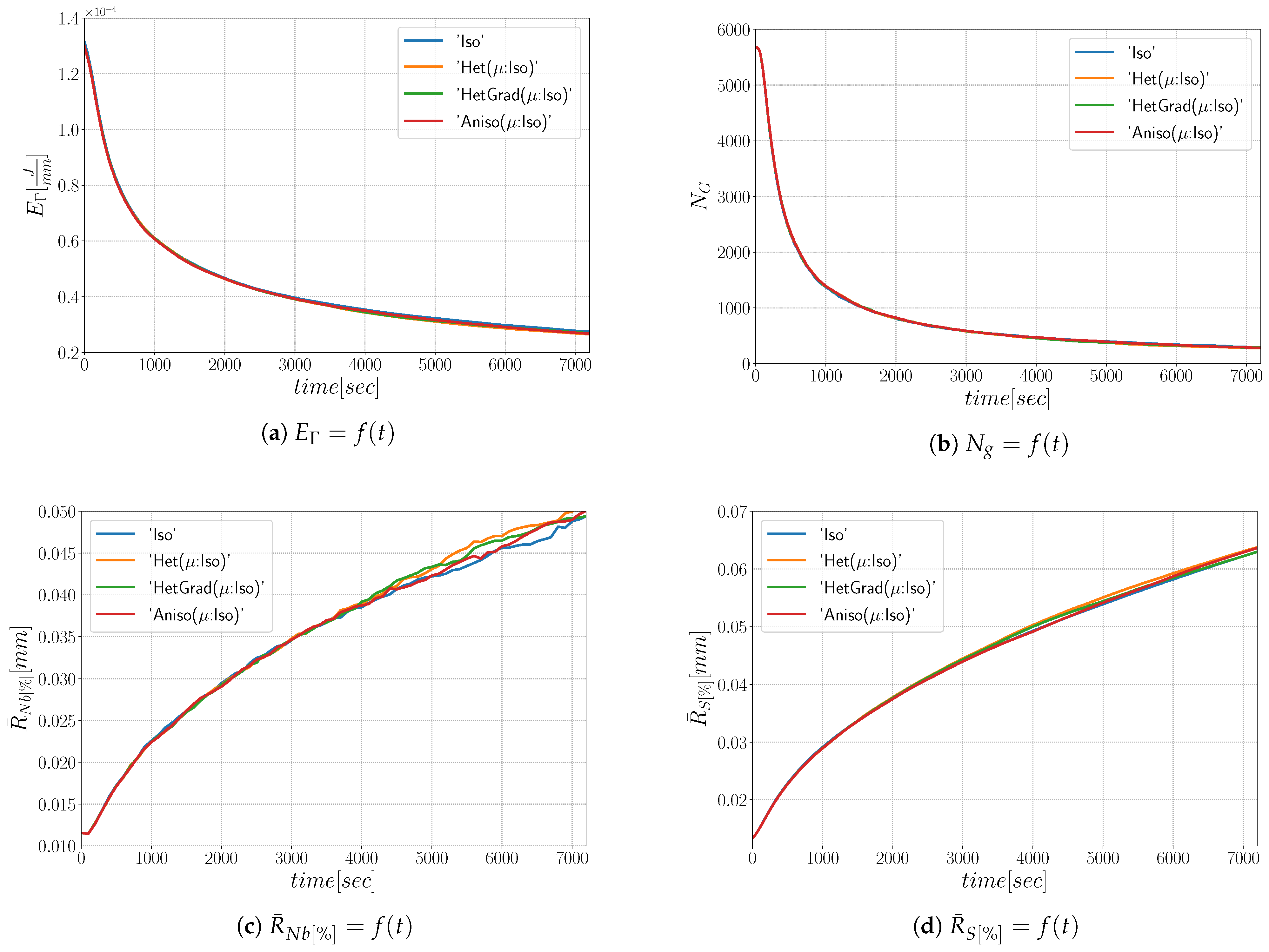
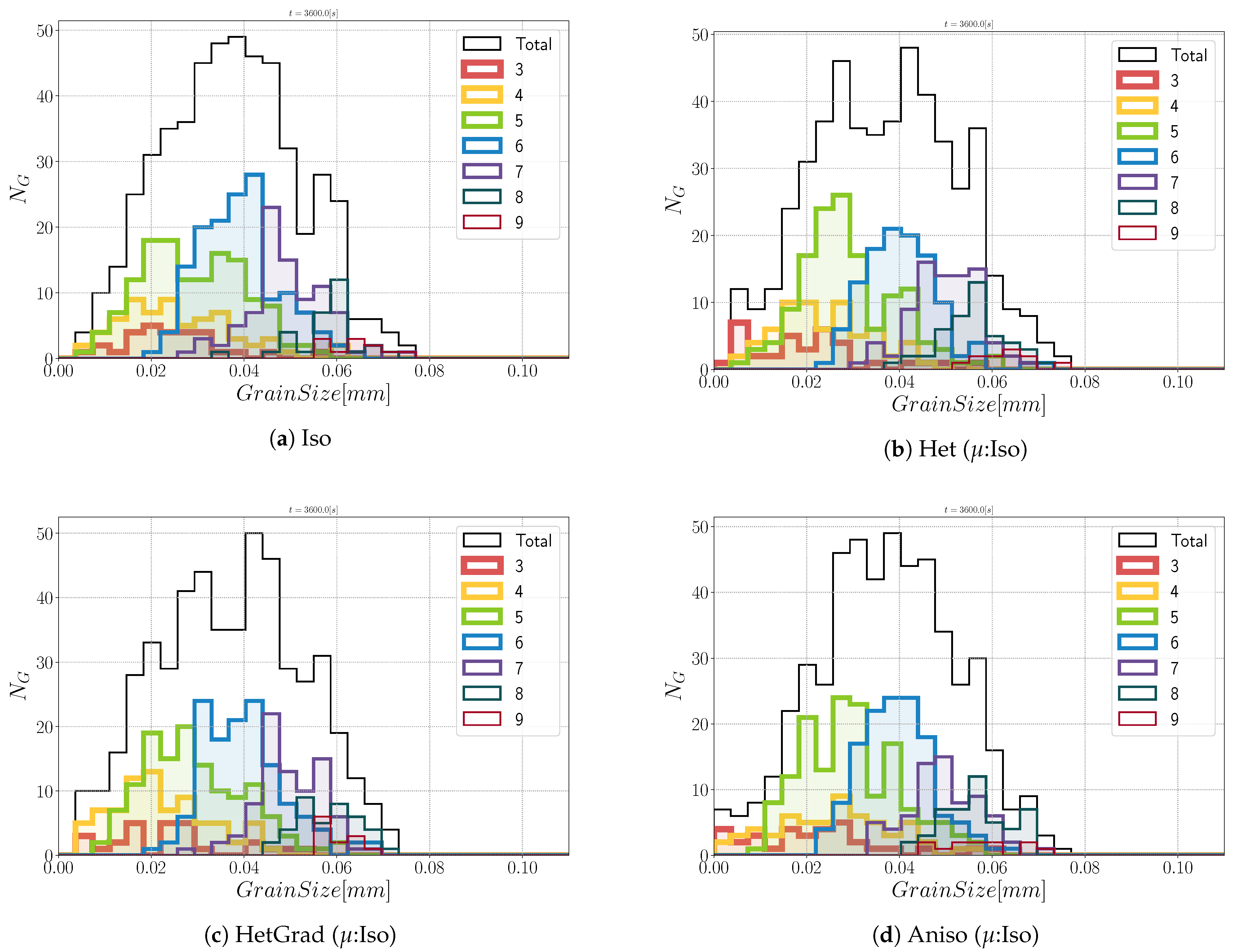
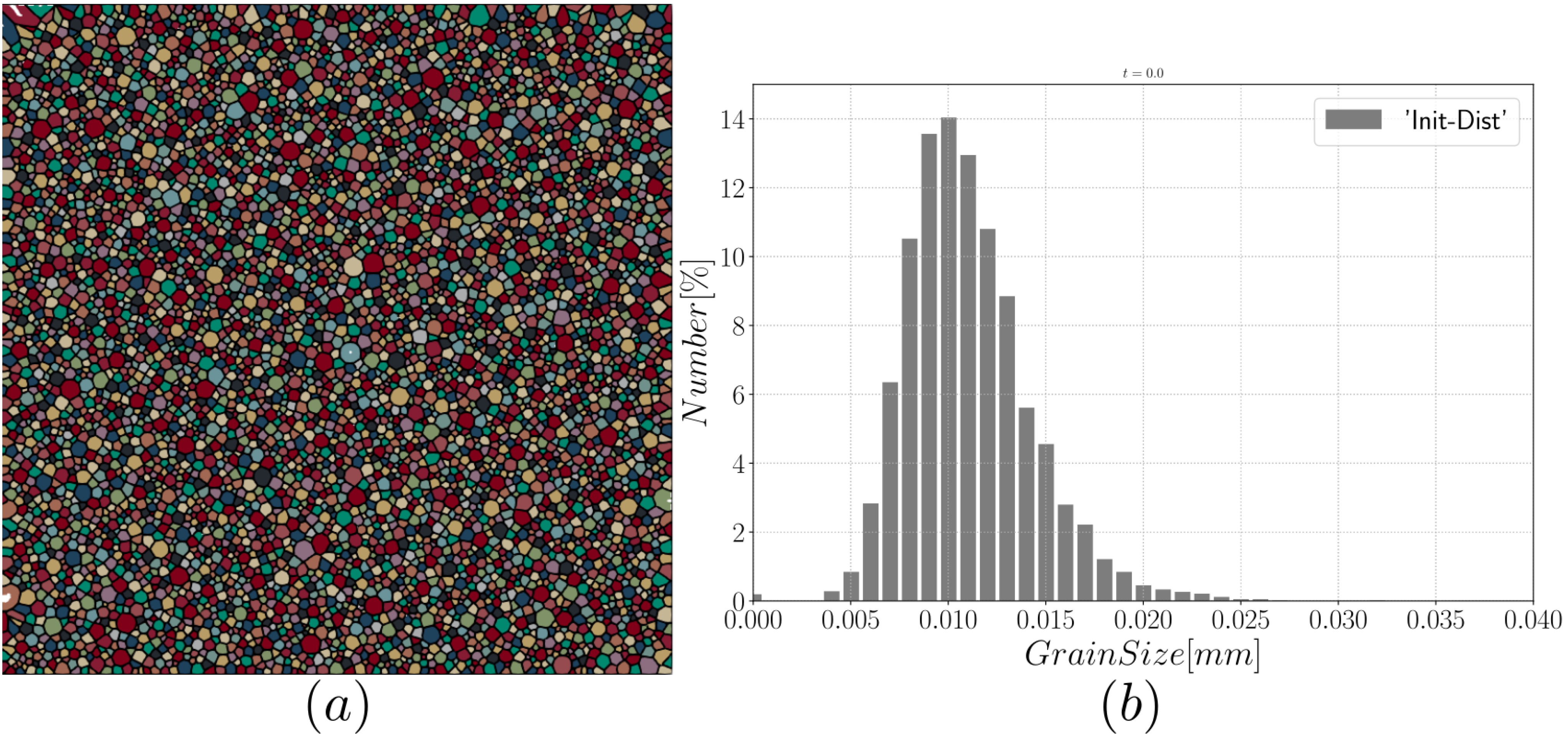
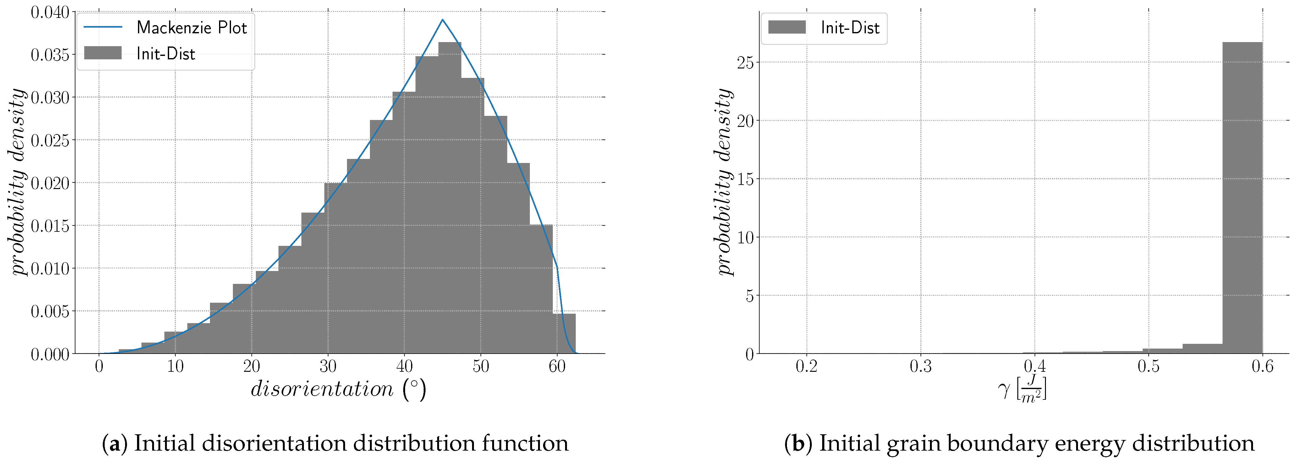
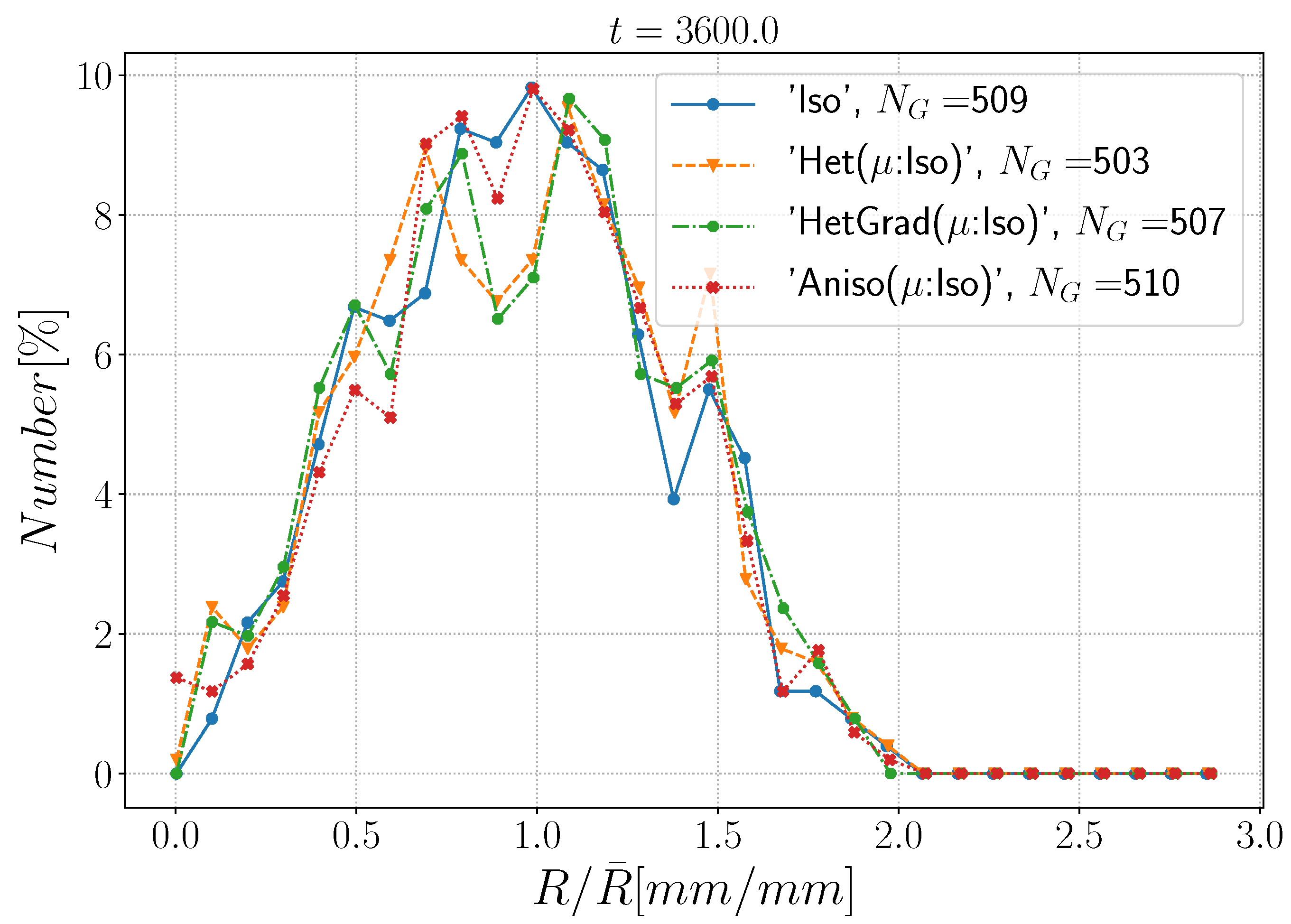
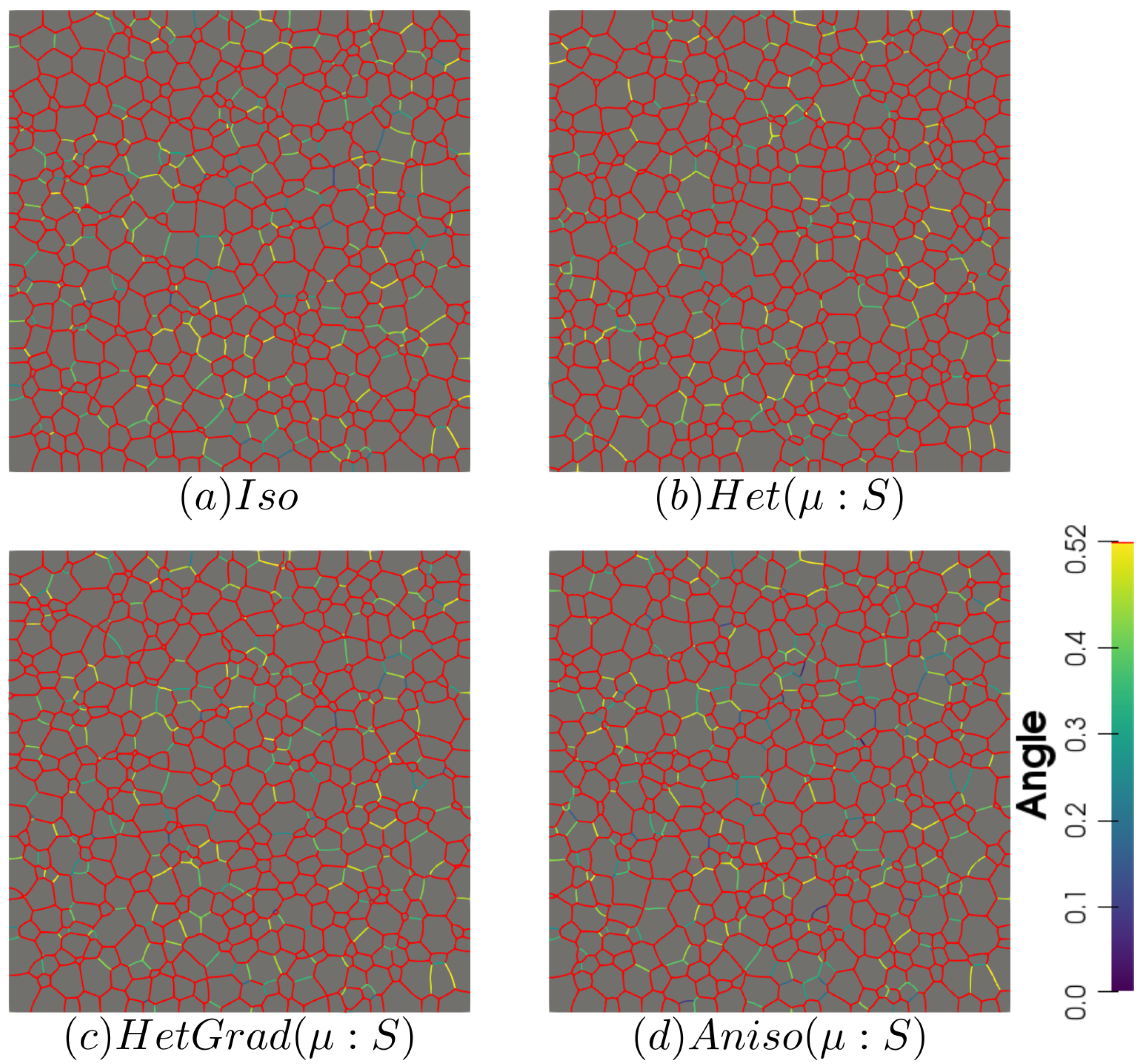
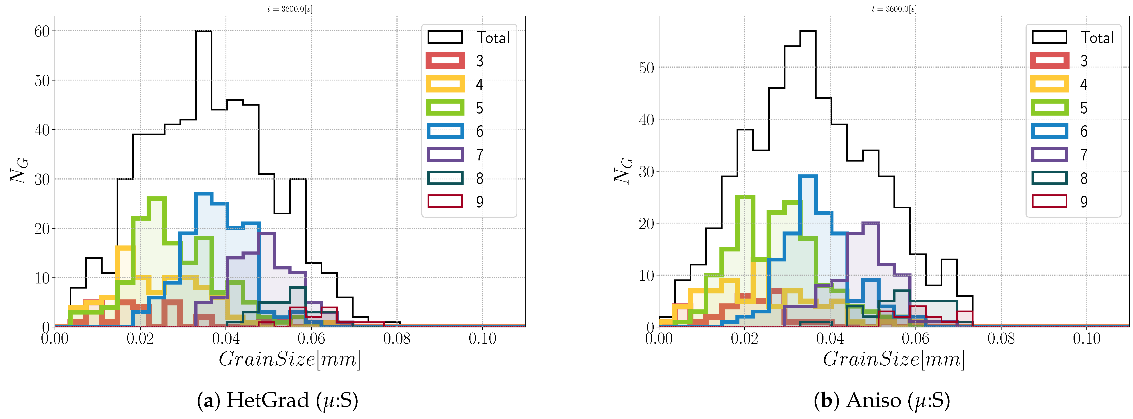
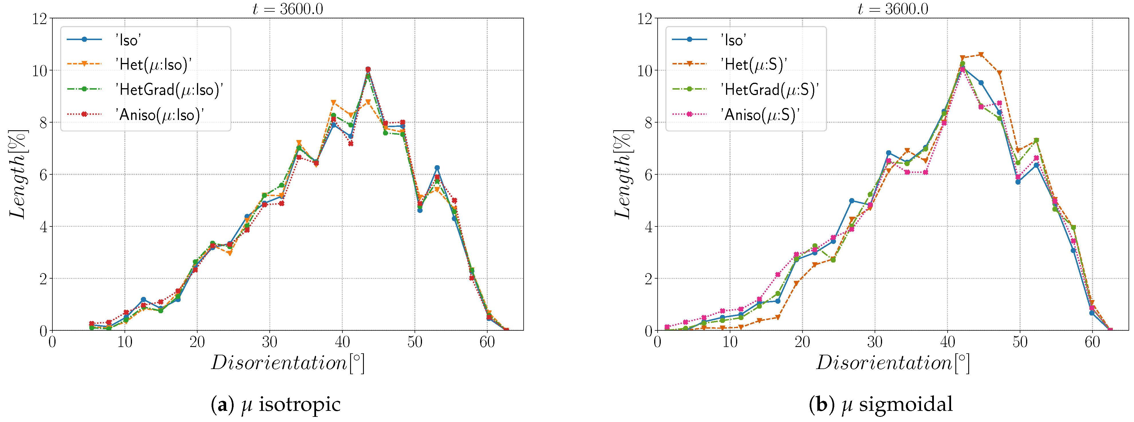
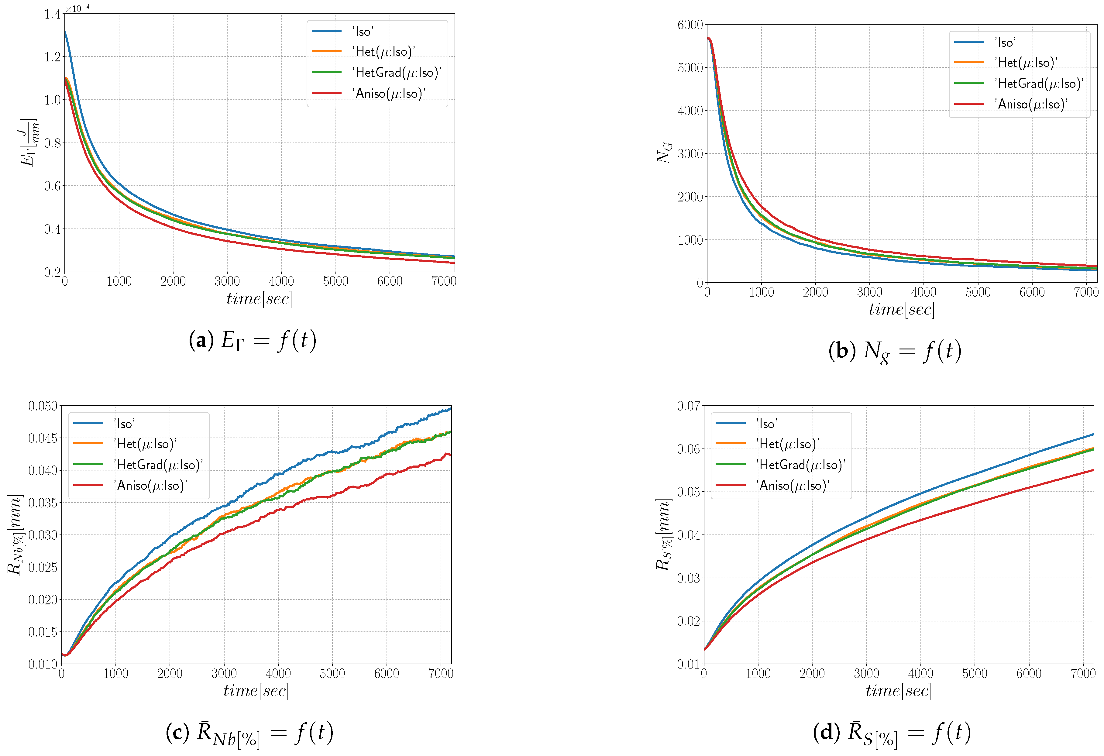
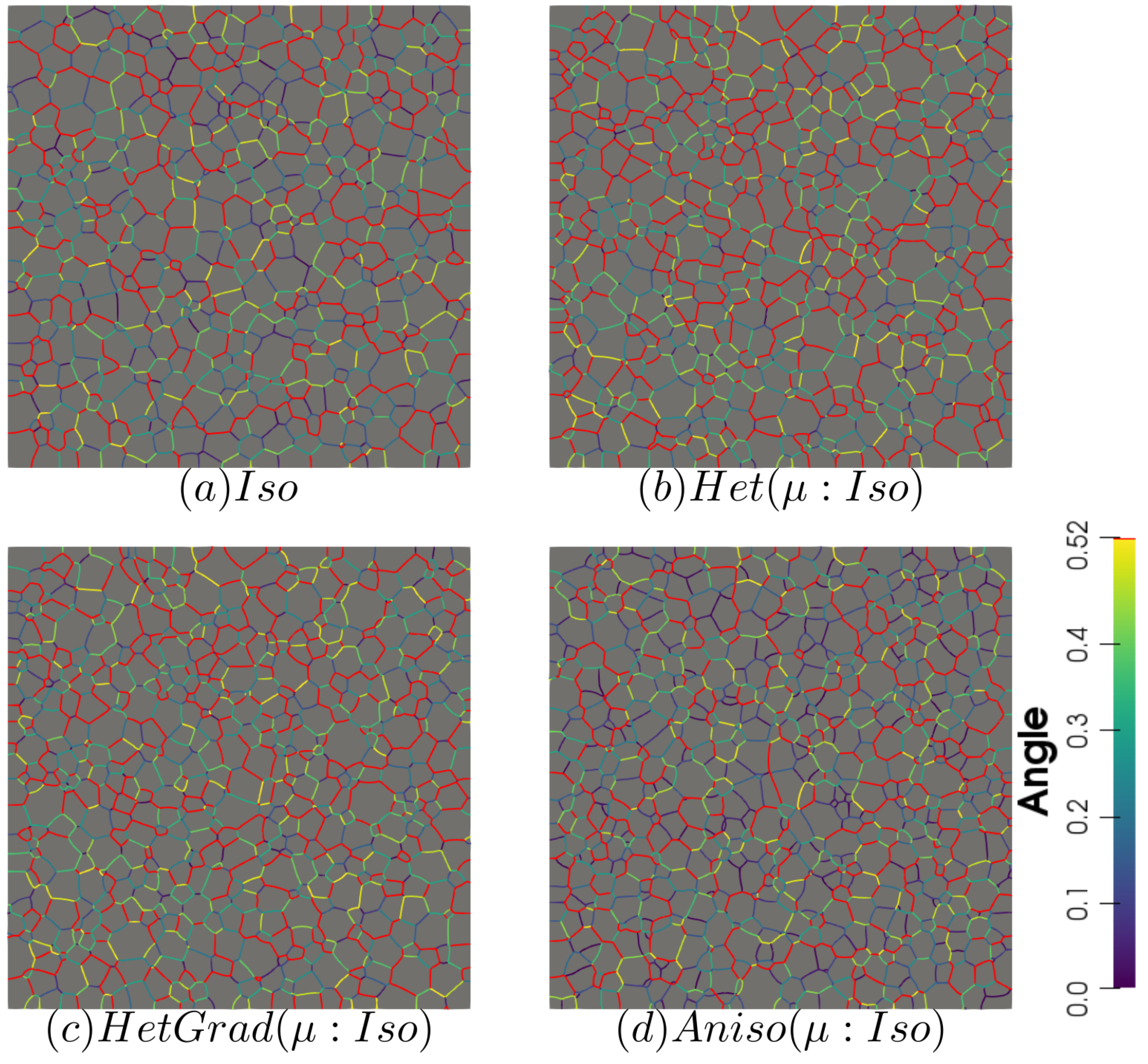
4. Effect of the Texture and Heterogeneous GB Properties during GG Simulations for a Polycrystalline Microstructure

In this section, we study a representative GB network in 2D. Figure 11 exhibits the initial characteristics of the microstructure, it consists of a square domain with length ${\displaystyle L=1.6}$ mm and 5000 grains generated using a Laguerre-Voronoi tessellation [52] based on an optimized sphere packing algorithm [53] with a log-normal distribution for the arithmetic mean grain size. The grain size, ${\displaystyle R}$, of each grain is defined as ${\displaystyle \sqrt{S/\pi }}$, with ${\displaystyle S}$ as its surface (i.e., defined as the radius of the equivalent circular grain of the same surface). Anisotropic re-meshing is used following Equation (27), with a refinement close to the interface, the mesh size in the tangential direction (as well as far from the interface) is fixed at ${\displaystyle h_t=5\mathsf{\mu }}$m and at ${\displaystyle h_n=1\mathsf{\mu }}$m in the normal direction. The time step is fixed at ${\displaystyle \Delta t=10}$s. This section is mainly devoted to studying the heterogeneity of both GB energy and mobility using the four introduced grain growth formulations. Finally, the same study is performed using a different texture in Appendix B.1.

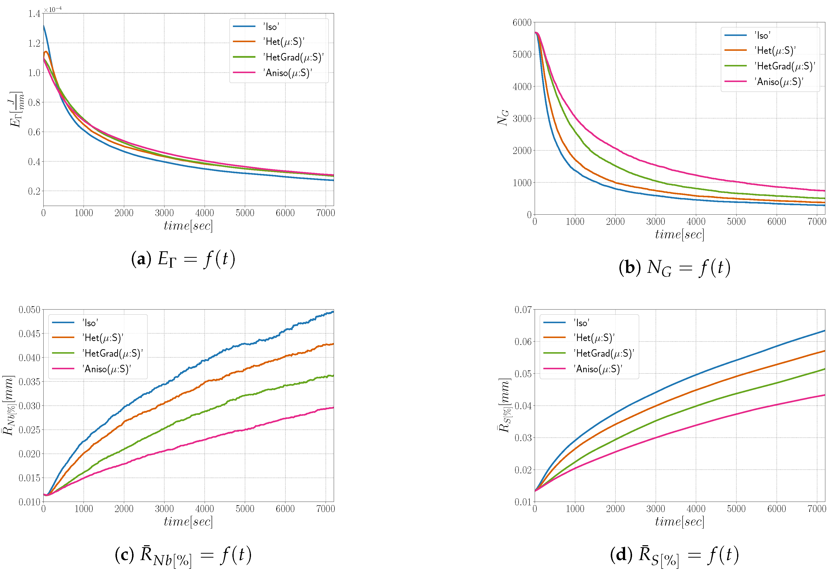
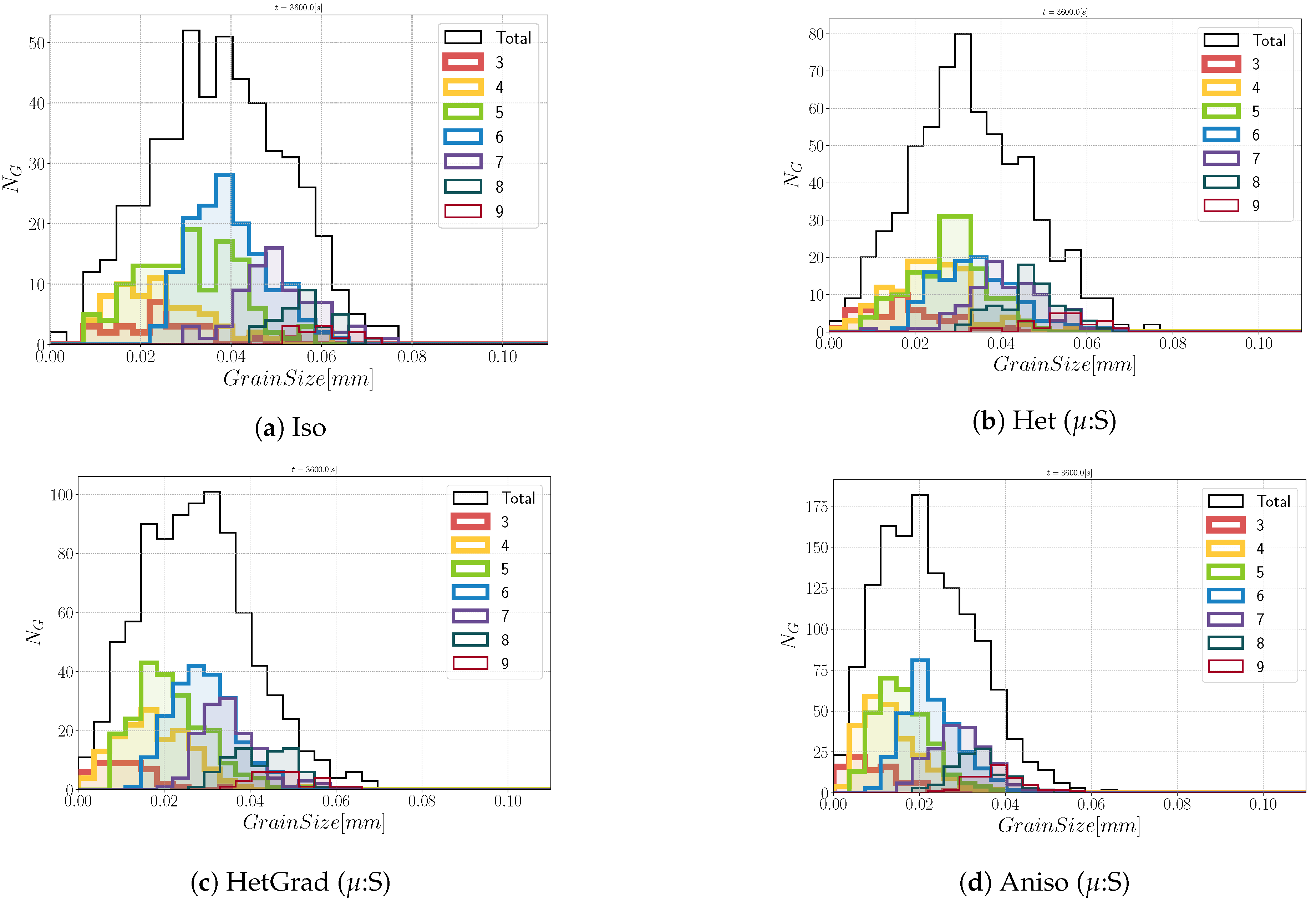
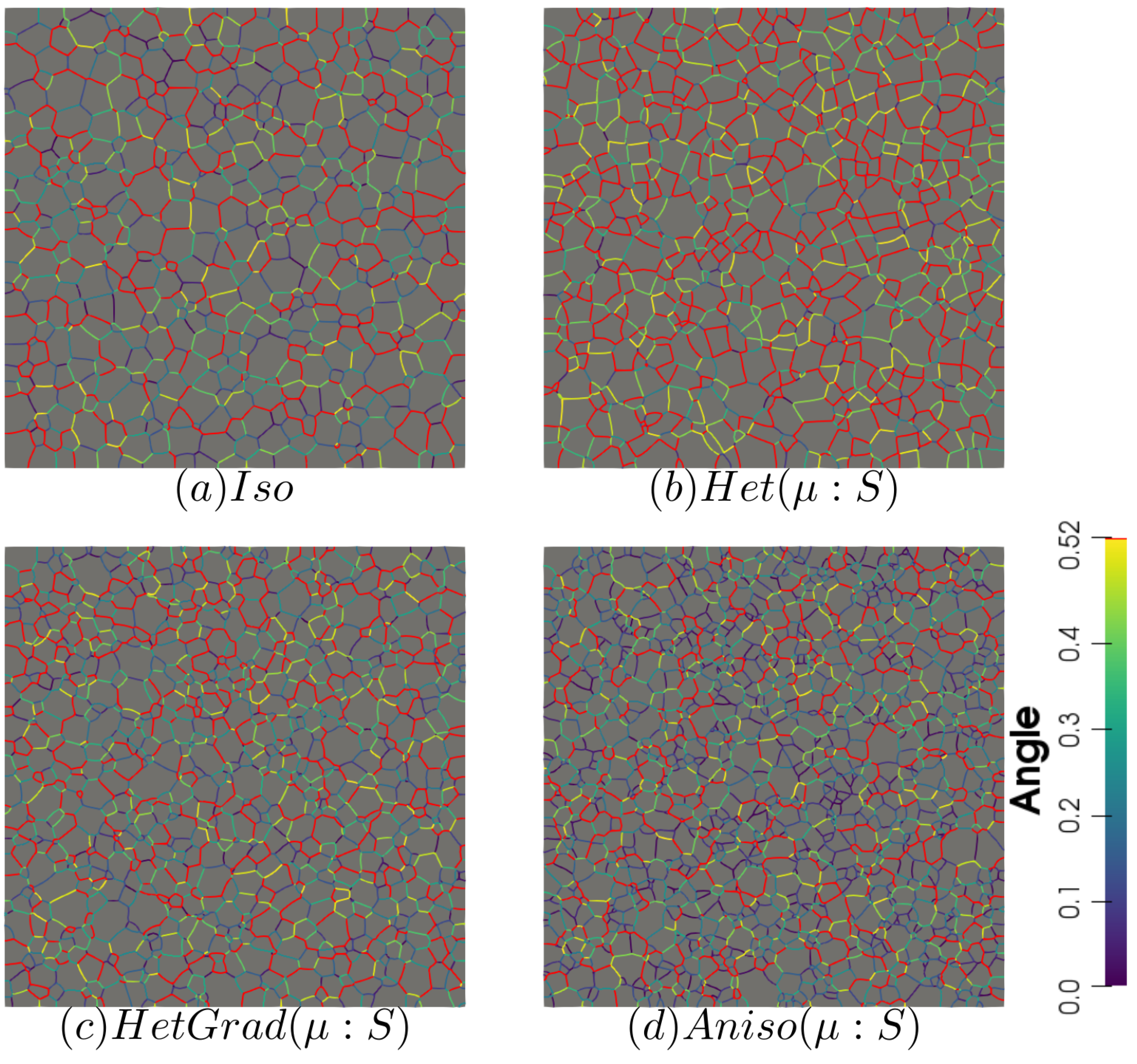
4.1. Effect of the Heterogeneity

Here, we use a mis-orientation-dependent GB energy and mobility, defined respectively with a Read–Shockley (RS) function [54] and a Sigmoidal (S) function, proposed by Humphreys in [55]:

$$\begin{array}{c}\hfill \left\{\begin{array}{c}\gamma \left(\theta \right)={\gamma }_{max}\frac{\theta }{{\theta }_0}\left(1-ln\left(\frac{\theta }{{\theta }_0}\right)\right),\theta <{\theta }_0\hfill \\ {\gamma }_{max},\theta \ge {\theta }_0\hfill \end{array}\right.\end{array}$$

(28)

$$\begin{array}{c}\hfill \mu \left(\theta \right)={\mu }_{max}\left(1-exp\left(-5{\left(\frac{\theta }{{\theta }_0}\right)}^4\right)\right),\end{array}$$

(29)

where ${\displaystyle \theta }$ is the disorientation, ${\displaystyle {\mu }_{max}}$ and ${\displaystyle {\gamma }_{max}}$ are the maximal GB mobility and energy respectively, and ${\displaystyle {\theta }_0={30}^{\circ }}$ is the disorientation defining the transition from a low-angle grain boundary (LAGB) to a high-angle grain boundary (HAGB). ${\displaystyle {\theta }_0}$ is normally considered to be between 15 and 20${\displaystyle {}^{\circ }}$, but here, this parameter is exaggerated to exacerbate the heterogeneity of the system. The maximal values for the GB properties are ${\displaystyle {\mu }_{max}=1.379}$ mm${\displaystyle {}^4}$ J${\displaystyle {}^{-1}}$ s${\displaystyle {}^{-1}}$, and ${\displaystyle {\gamma }_{max}}$ = 6 ${\displaystyle \times }$ 10${\displaystyle {}^{-7}}$ J mm${\displaystyle {}^{-2}}$, and are typical for a stainless steel [56].

Figure 12 shows the orientation field using the vector magnitude ${\displaystyle O_G=\sqrt{{\phi }_1^2+{\varphi }^2+{\phi }_2^2}}$, where ${\displaystyle ({\phi }_1,\varphi ,{\phi }_2)}$ are the three Euler angles. The Euler angles defining the crystallographic orientations generated in this case are generated randomly, leading to a Mackenzie-like disorientation distribution function [57]. As the Read–Shockley model is used to define ${\displaystyle \gamma }$, the GB energy is concentrated at high values, as illustrated in Figure 13.

4.1.1. Heterogeneous Grain Boundary Energy

In this section, GB energy is defined using Equation (28) and GB mobility is assumed isotropic. Hence, the Het, HetGrad, and Aniso formulations are presented as “Het(${\displaystyle \mu }$:Iso)”, “HetGrad(${\displaystyle \mu }$:Iso)”, and “Aniso(${\displaystyle \mu }$:Iso)”. The results are summarized in Figure 14, Figure 15 and Figure 16. First, it is noticeable that all the formulations have a similar evolution concerning the total grain boundary energy ${\displaystyle E_{\Gamma }}$, the number of grains ${\displaystyle N_g}$, and the mean grain size weighted by number ${\displaystyle {\overline{R}}_{Nb[\%]}}$ or by surface ${\displaystyle {\overline{R}}_{S[\%]}}$. Additionally, if the grain size distribution weighted by number is normalized (Figure 15), one can recognize that all the formulations have similar distributions and the minima have similar values with respect to the mean radius. Similar results for the “Iso” and “HetGrad” formulations with heterogeneous GB energy defined by the Read–Shockley model were already reported [19].

The slow evolution of the mean values has been reported as a consequence of little local-heterogeneity produced by a Mackenzie-like DDF and/or a low value of ${\displaystyle {\theta }_0}$ [31,35,58,59]. If the DDF starts as a Mackenzie distribution, the value of GB mobility and energy is focused at higher values, thus the microstructure cannot easily find a path to minimize its energy faster and the DDF changes slightly from its initial Mackenzie form. In other words, the initial configuration is almost isotropic. Slight differences can be observed after ${\displaystyle t=1}$ h for the different formulations, which may be due to the low final number of grains (${\displaystyle N_G\approx 500}$).

Regarding the morphology of the microstructures at ${\displaystyle t=1}$ h, the grains are equiaxed. If we divide the total group of grains in classes divided by the number of neighbors (defined as the coordination number in the following), ${\displaystyle n}$, an interesting analysis regarding the morphology of grains could be performed. In Figure 16, the contribution of every class is depicted, and at ${\displaystyle t=0}$ s, most of the grains verify ${\displaystyle n=5}$. After one hour, one can directly appreciate that the class with ${\displaystyle n=6}$ is the main class using the four formulations. This agrees with theoretical predictions of grain boundary motion with isotropic GB energy, which promotes triple junctions with dihedral angles near ${\displaystyle {120}^{\circ }}$ [60]. This aspect again illustrates the limited impact of the considered anisotropy in this configuration.

4.1.2. Heterogeneous Grain Boundary Energy and Mobility

In this section, both GB energy and mobility are heterogeneous, respectively defined with Equations (28) and (29), and for that reason, the names introduced above are replaced by “Het (${\displaystyle \mu }$:S)”, “HetGrad (${\displaystyle \mu }$:S)”, and “Aniso (${\displaystyle \mu }$:S)”. In order to compare the results presented above, the same initial microstructure and crystallographic orientations are used. The mean values’ evolution and distributions remain similar among the four formulations and retain similar values as presented before. The heterogeneous GB mobility may affect the morphology of the microstructure due to a retarding effect from boundaries with disorientation lower than ${\displaystyle {\theta }_0}$. There is similarity between the four microstructures shown in Figure 17, showing mostly equiaxed grains. Two important aspects of these microstructures are that the microstructure obtained by the “Het” formulation is the most dissimilar, with a lower number of boundaries with disorientation inferior to ${\displaystyle {\theta }_0}$. Second, the presence of low-angle boundaries (${\displaystyle \theta <{30}^{\circ }}$) looks higher using the Anisotropic formulation. Nevertheless, this is not reflected in the interfacial energy evolution nor the DDF (see Figure 18).

Finally, Figure 19 shows the disorientation distribution function using both an isotropic and heterogeneous mobility at ${\displaystyle t=1}$ h. As stated before, the initial Mackenzie-type distribution evolves slowly, and a slow preference of low-angle boundaries is found. Using heterogeneous mobility slightly affects the DDF, and one can see that the Anisotropic formulation (Aniso (${\displaystyle \mu }$:S)) exacerbates low values of disorientation reflected in higher values in the distribution at ${\displaystyle 0<\theta <{10}^{\circ }}$. Due to the Mackenzie-like DDF, the GB energy distribution is concentrated around ${\displaystyle {\gamma }_{max}}$, leading to microstructures with triple junction angles around ${\displaystyle {120}^{\circ }}$ (see Figure 17). These results are in accordance with prior works [58,60,61].

At this point, one can see that for a non-textured polycrystal with an initial Mackenzie-like DDF, the evolution of the GB network and of the GB energy and mobility fields are similar to an isotropic case. That is the fundamental reason explaining the weak differences among the results of the different formulations. The results exhibit similar evolution of mean values, distributions, and grains’ morphology. In order to study the behavior of the different formulations for a wider spectrum of GB properties, Appendix B.1 is devoted to studying the effect of a strong texture using the four formulations with isotropic and heterogeneous mobility. Under the effect of a textured microstructure, the Anisotropic formulation seems to be the more physical by promoting a higher percentage of boundaries with lower values of disorientation.

4.2. CPU Time

All the performed polycrystalline simulations were considered on 20 cores with the same mesh size, ${\displaystyle h_n=1\mathsf{\mu }}$m, in the normal direction of the interface, and ${\displaystyle h_t=5\mathsf{\mu }}$m in the tangential direction of the interface and far from the interface. As expressed earlier, both heterogeneous formulations and the Anisotropic formulation have additional terms which can be synonymous of more complex resolutions. This aspect, if not significant when moderated by anisotropy, is considered, as illustrated in the first line of

Table 1. CPU time in hours of the four formulations with heterogeneous GB energy and mobility.

Case	Iso	Het	HetGrad	Aniso
Random	5.4	5.5	5.5	5.6
Textured	5.4	5.5	7.3	9.4

.

However, the CPU time changes significantly for the textured case presented in Appendix B.1. The HetGrad and Aniso formulations present, respectively, an increase of 35% and of 74% of the calculation time, in comparison to the Isotropic formulation.

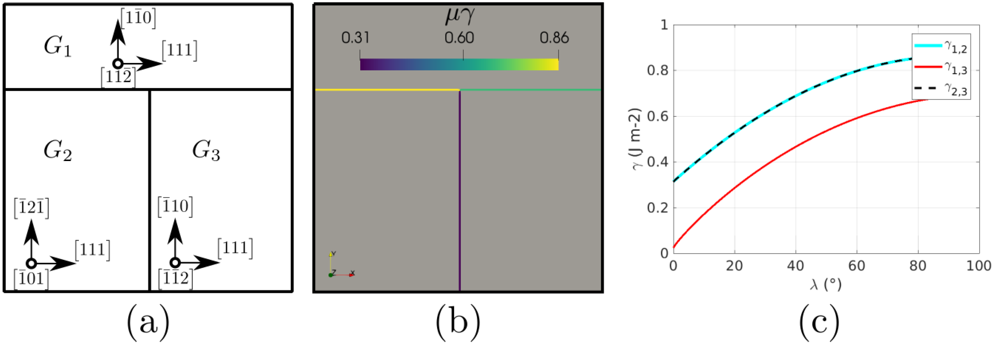
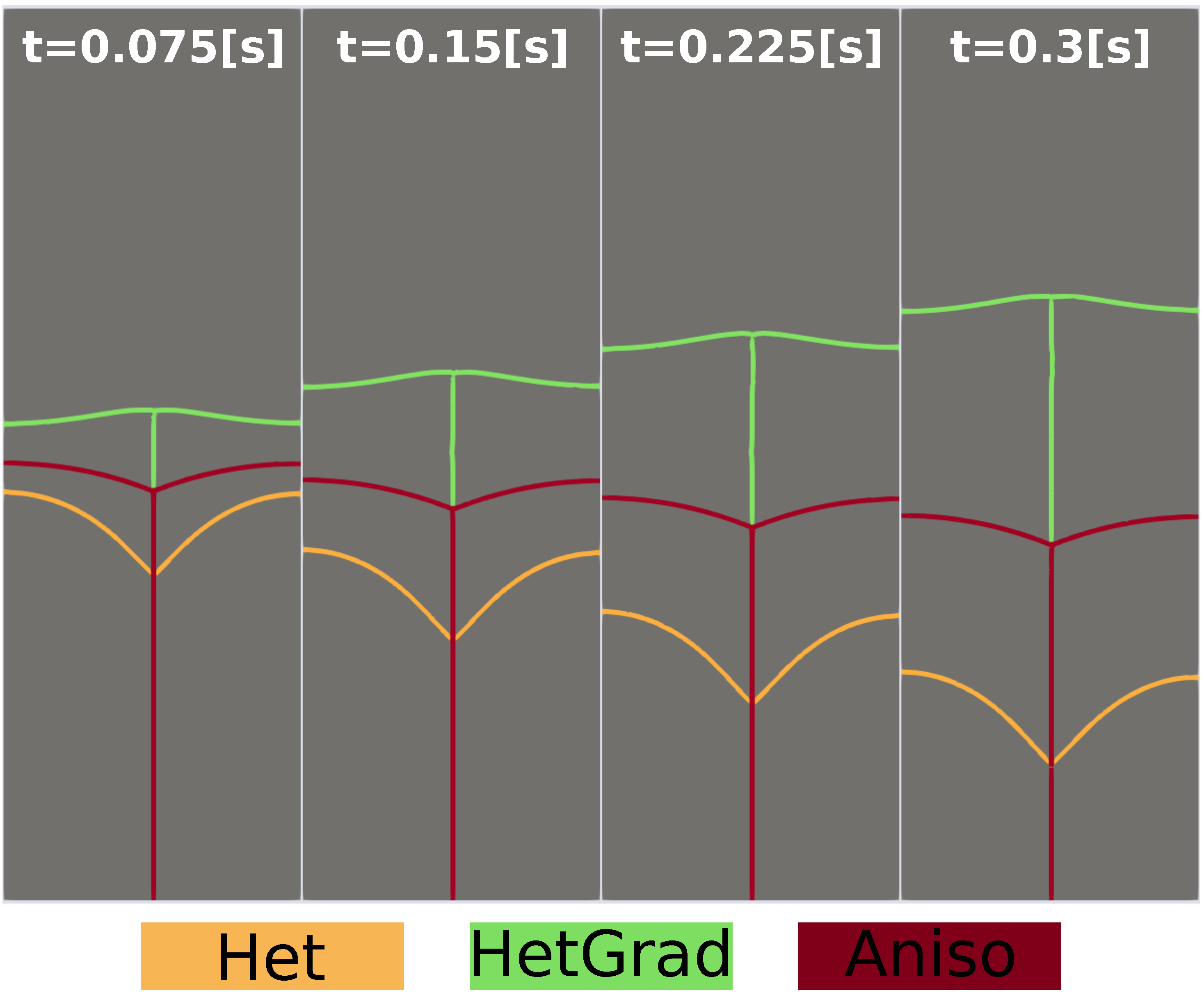
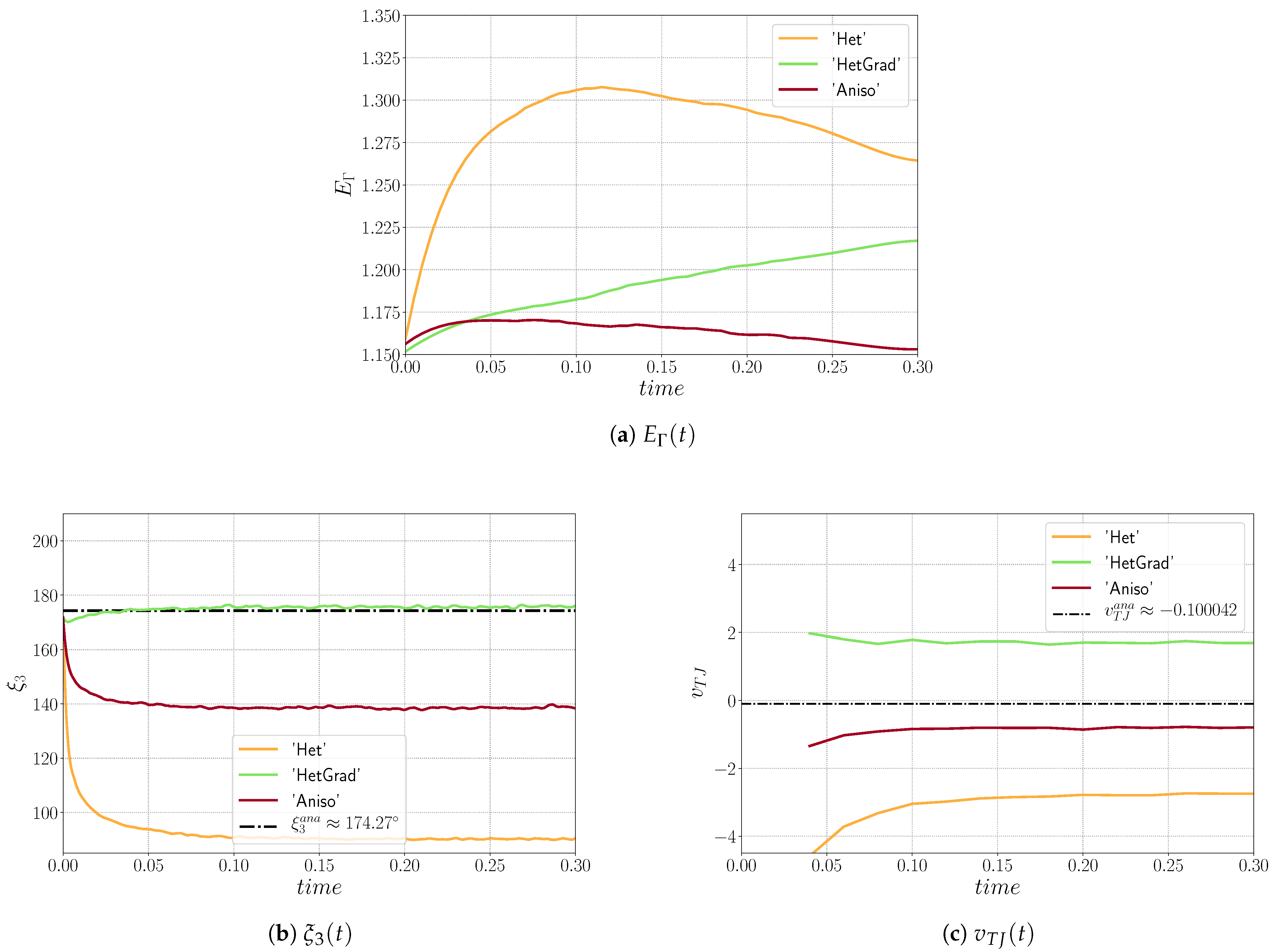
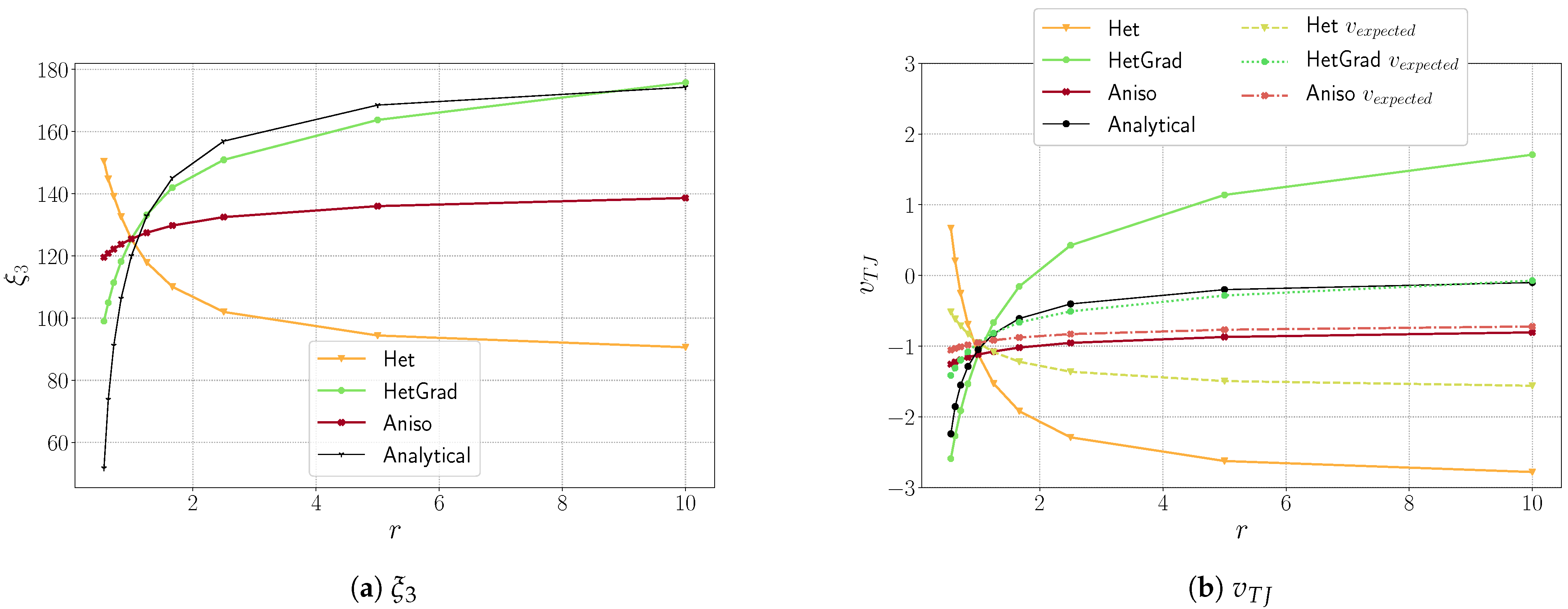
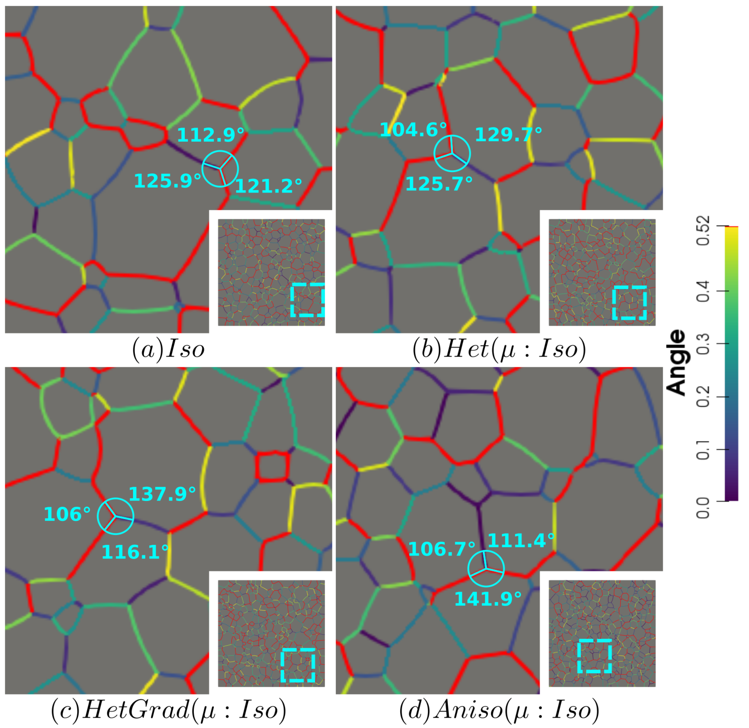
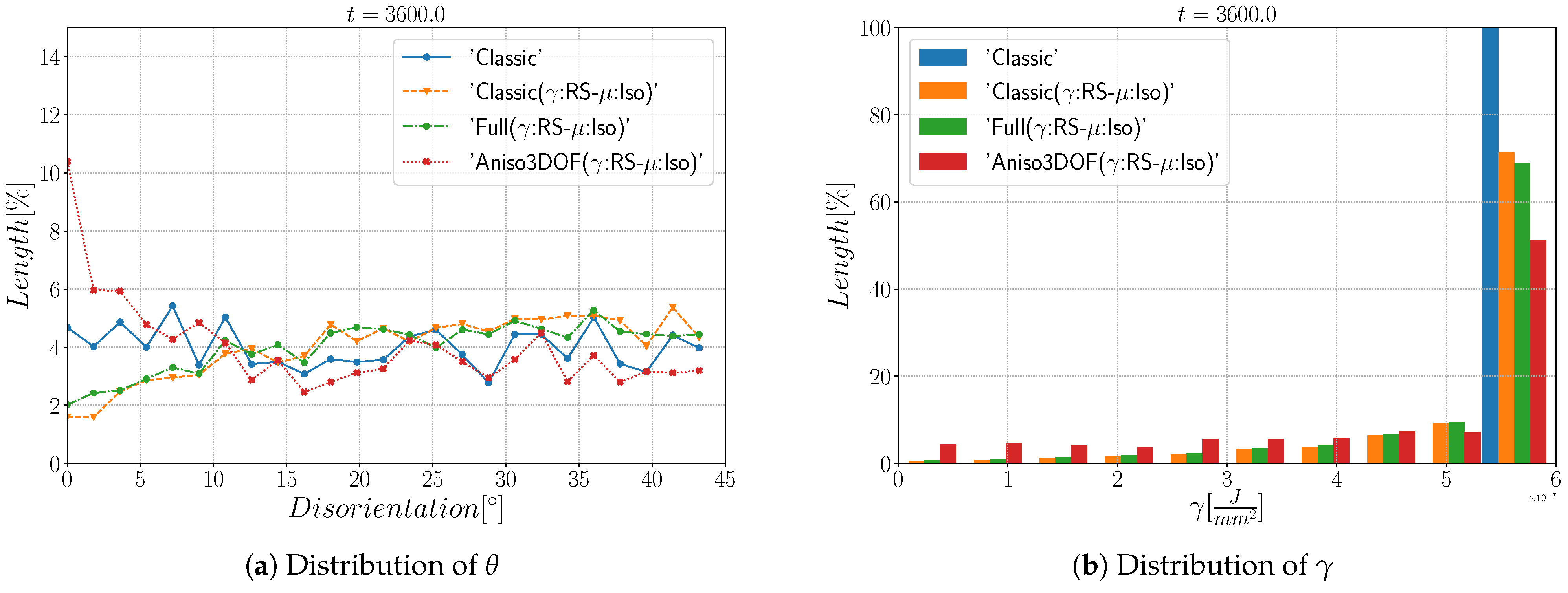
5. Accounting for Mis-Orientation and Inclination Dependence

The formulations presented above have dealt with heterogeneous GB properties. However, we know that the nature of the GB is described in a 5D space generated by the inclination and the mis-orientation. The effect of the normal direction has been described by Herring in [62] as a torque term. Hence, a triple junction should respect a condition frequently known as Herring’s equation, Equation (20).

Due to the high dimensional space of GBs, many researchers have attempted to propose metrics that properly represent symmetries [63,64,65,66,67,68,69]. With these metrics, one can compare and compute the shortest paths (geodesics) between GBs. As the mis-orientation and the normal orientation can change during the microstructure evolution due to grain rotation or grain disappearance/appearance, the evolution of the metric could reveal important information about the structure–property relationship. Recent works by Chesser et al. and Francis et al. have proposed new metrics using octonions [70,71], revealing good predictions of GB energy of the data published by Olmsted in [72]. To the authors’ knowledge, the effect of the GB normal orientation is not clear, and more experimental, numerical, and theoretical works are needed. Here, we define the effect of the normal orientation using a model of GB energy proposed for fcc metals by Bulatov et al. [73] and available in the GB5DOF code. When ${\displaystyle \gamma }$ is defined using the GB5DOF code, both the effect of the mis-orientation and inclination are taken into account using the crystallographic orientations of the two adjacent grains and the local coordinate system of the corresponding GB [73].

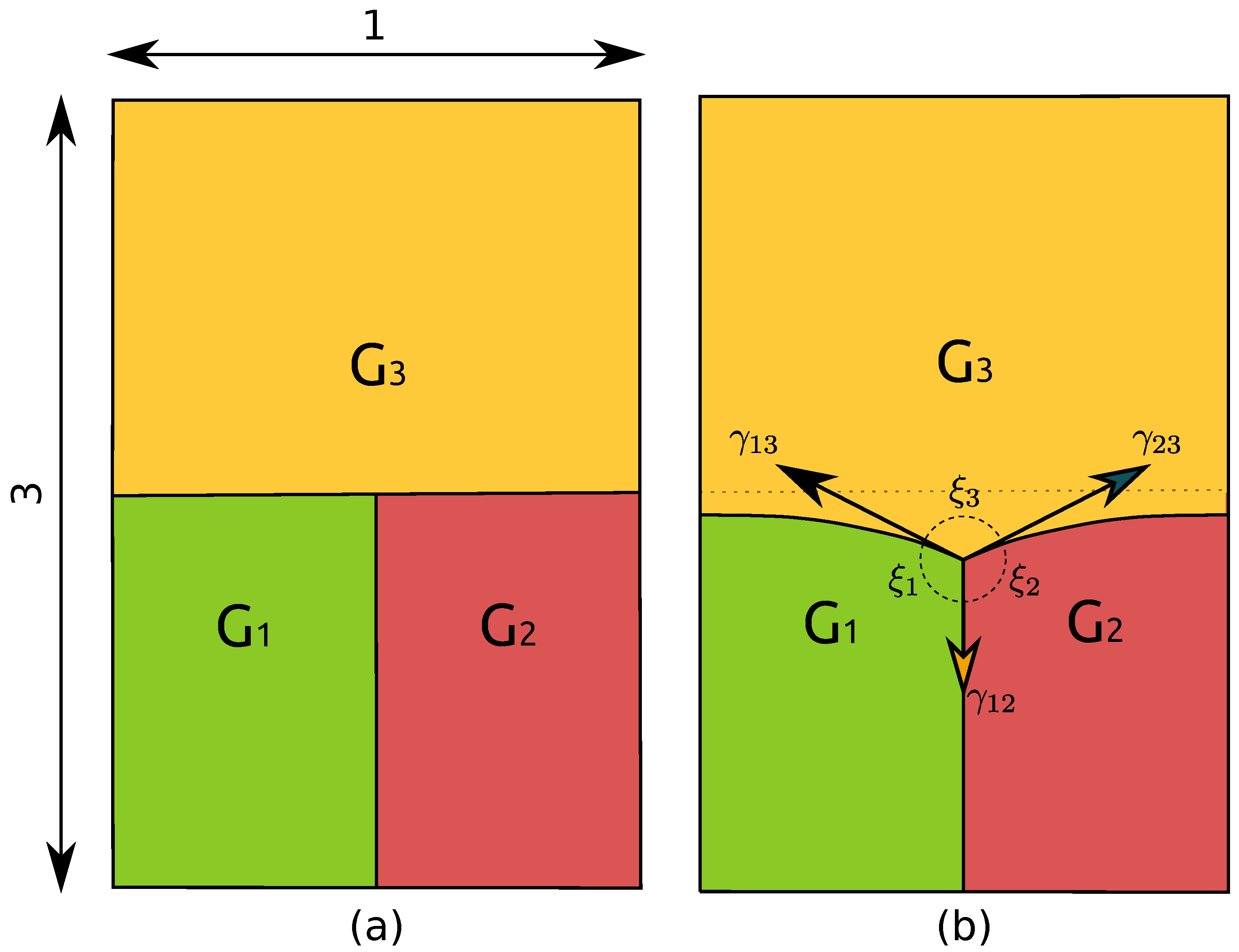
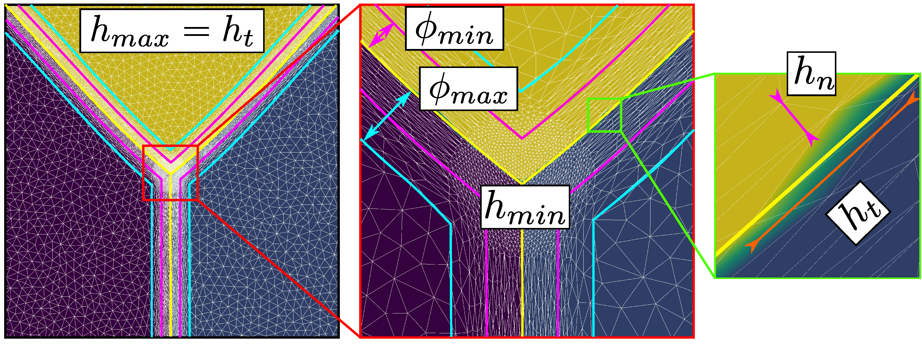
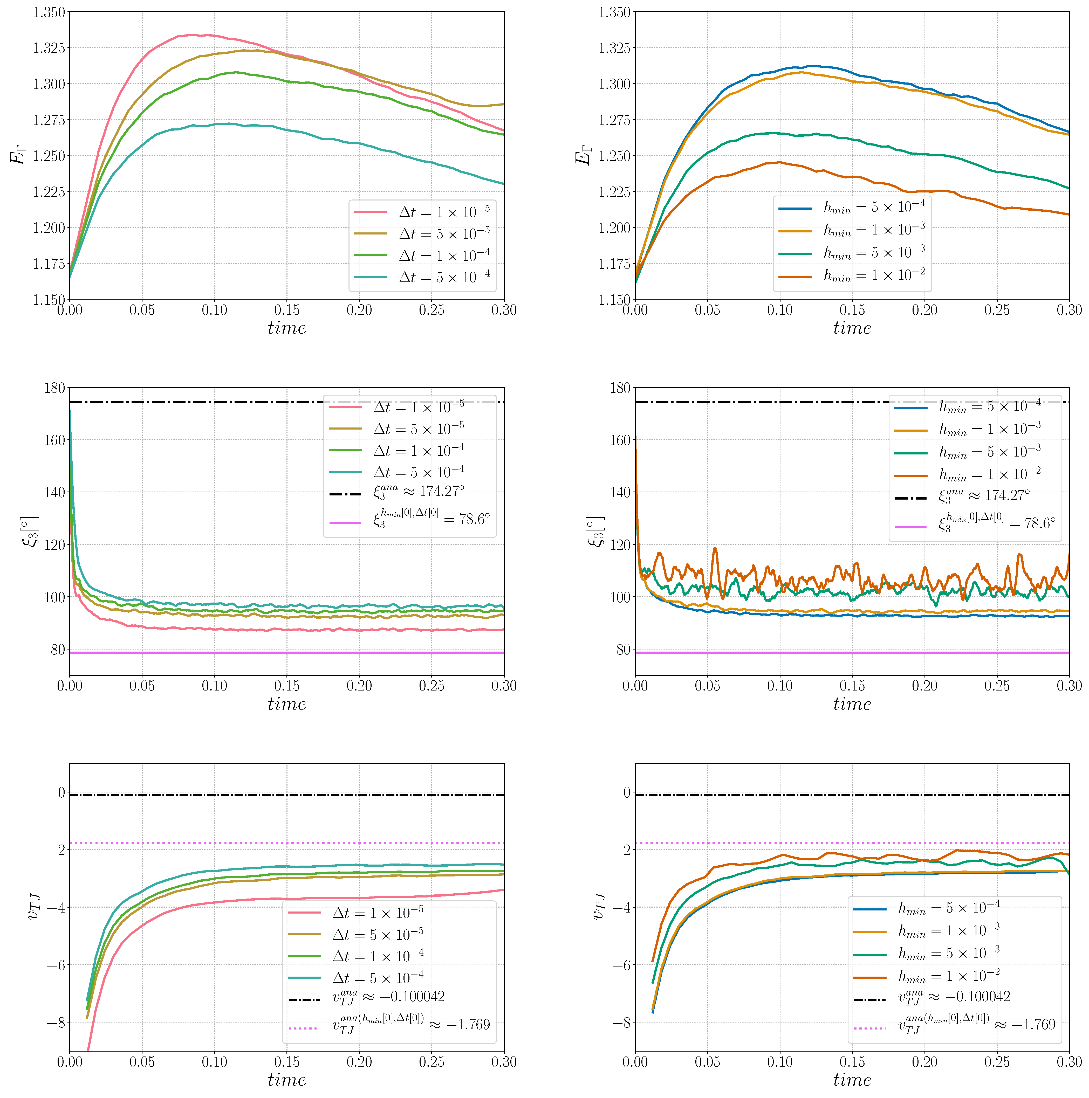
5.1. Triple Junction

This case again consists of a triple junction, as described by Figure 20. We performed simulations with a constant GB mobility set to ${\displaystyle \mu }$ = 1 ${\displaystyle \times }$ 10${\displaystyle {}^6}$ mm${\displaystyle {}^4}$ J${\displaystyle {}^{-1}}$ s${\displaystyle {}^{-1}}$, taken from [74], a domain of ${\displaystyle 1\times 1}$ mm${\displaystyle {}^2}$, and a time step of ${\displaystyle \Delta t}$ = 5 ${\displaystyle \times }$ 10${\displaystyle {}^{-5}}$ s. The Aniso formulation is used by considering ${\displaystyle \gamma }$ as only initially defined by the mis-orientation and then also dependent on the inclination (obtained through the GB5DOF code and denoted as Aniso-GB5DOF). The Iso, Het, and HetGrad are not presented here because they evolve in the wrong direction (the expected movement should reduce the length of the interface between grain ${\displaystyle G_1}$ and ${\displaystyle G_2}$, depicted in yellow). The evolution of the interfaces shown in Figure 21 presents similar tendencies to the cases presented by Garcke in [75] and Hallberg in [34]. If both evolutions (without or with the inclination dependence) seem to promote similar triple junction evolution, the Aniso-GB5DOF case exhibits a much faster evolution, which illustrates the importance of accounting for the inclination in the reduced mobility description.

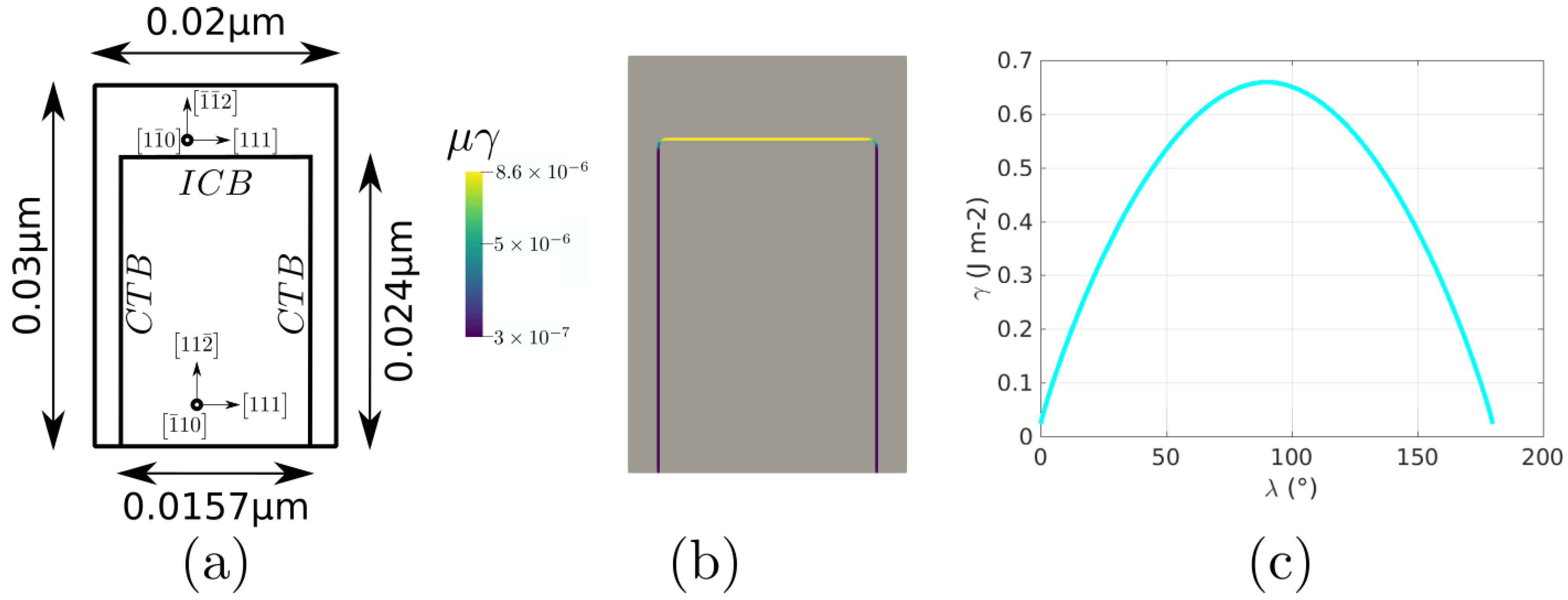
5.2. Coherent and Incoherent Twin Boundary

The main advantage of the GB5DOF code is that it is possible to characterize coherent and incoherent twin boundaries. These special GBs play an important role on polycrystalline microstructures, and their modeling is not frequently discussed at the mesoscopic scale. The next example was firstly proposed by Brown and Ghoniem in [76] and also reproduced at the mesoscopic scale in [34]. It consists of two grains composed of two coherent twin boundaries (CTB) and one incoherent boundary (ICB). Figure 22 shows the crystallographic orientation, the initial GB energy, and the variation of the GB energy as a function of the GB inclination. The Iso and Aniso formulations were used to model the GB movement. For the Aniso formulation, the GB5DOF code was used to compute the GB energy all along the simulation. On the other hand, the GB energy of the Iso case is constant and set to ${\displaystyle \gamma }$ = 0.65969 J m${\displaystyle {}^{-2}}$. The evolution of the GB is shown in Figure 23. The time step was set to ${\displaystyle \Delta t}$ = 0.1 ns and GB mobility was set to ${\displaystyle \mu }$ = 1.3 ${\displaystyle \times }$ 10${\displaystyle {}^7}$${\displaystyle \mathsf{\mu }}$m${\displaystyle {}^4}$ J${\displaystyle {}^{-1}}$ ns${\displaystyle {}^{-1}}$ in order to reproduce the velocity of the ICB found by Brown and Ghoniem in [76], ${\displaystyle v_{ICB}}$ = 1.2 m s${\displaystyle {}^{-1}}$. The movement of the ICB should be uniform and it should respect the flatness of the CTB. The Aniso-GB5DOF simulation enables to respect the expected behavior.

6. Conclusions

Different FE-LS formulations to simulate grain growth were presented and compared in this text, with the isotropic formulation, in which the grain boundary mobility and energy are assumed constants, being the most used framework in the literature. The isotropic formulation is able to reproduce mean grain size and grain size distribution evolutions when a moderated anisotropy is involved.

From the results presented using the triple junction cases, the Anisotropic formulation was the most accurate. The triple junction velocity predictions were the closest to the theoretical values while predicting accurate dihedral angles. In addition, the interfacial energy was always minimized and faster compared to the other approaches.

Additionally to these academic configurations, simulations using two different polycrystalline microstructures were performed. First, the initial orientations were generated using a uniform distribution, producing an initial Mackenzie-like disorientation distribution. Finally, another example with a textured orientation was considered. It was then illustrated that for a simple microstructure with initial random orientation, an isotropic formulation can be used, and that for a textured configuration, the Anisotropic formulation presents the best behavior in terms of grain morphology, DDF, and interfacial energy evolution predictions, while keeping a reasonable efficiency, compared to the isotropic formulation.

It was also illustrated that the Anisotropic approach is the most versatile approach, enabling to take into account the inclination dependence. Future works will be focused on the use of 2D and 3D experimental results concerning 304L and 316L, which are currently capitalized. These experimental results will be used to validate the Anisotropic formulation with more complex datasets.

References

1. Humphreys, F.J.; Hatherly, M. Recrystallization and Related Annealing Phenomena; Elsevier: Amsterdam, The Netherlands, 2012. [Google Scholar]
2. Watanabe, T. Grain boundary engineering: Historical perspective and future prospects. J. Mater. Sci. 2011, 46, 4095–4115. [Google Scholar] [CrossRef]
3. Zhang, L.; Han, J.; Xiang, Y.; Srolovitz, D.J. Equation of Motion for a Grain Boundary. Phys. Rev. Lett. 2017, 119, 246101. [Google Scholar] [CrossRef] [Green Version]
4. Zhu, Q.; Cao, G.; Wang, J.; Deng, C.; Li, J.; Zhang, Z.; Mao, S.X. In situ atomistic observation of disconnection-mediated grain boundary migration. Nat. Commun. 2019, 10, 1–8. [Google Scholar] [CrossRef] [PubMed] [Green Version]
5. Wang, M.; Dake, J.; Schmidt, S.; Molodov, D.; Krill, C., III. Reverse engineering the kinetics of grain growth in Al-based polycrystals by microstructural mapping in 4D. In Proceedings of the 40th Risø International Symposium on Materials Science, Harry Bhadeshia, Denmark, 2–6 September 2019. [Google Scholar]
6. Garcke, H.; Nestler, B.; Stoth, B. A multiphase field concept: Numerical simulations of moving phase boundaries and multiple junctions. SIAM J. Appl. Math. 1999, 60, 295–315. [Google Scholar] [CrossRef] [Green Version]
7. Miyoshi, E.; Takaki, T. Multi-phase-field study of the effects of anisotropic grain-boundary properties on polycrystalline grain growth. J. Cryst. Growth 2017, 474, 160–165. [Google Scholar] [CrossRef]
8. Moelans, N.; Wendler, F.; Nestler, B. Comparative study of two phase-field models for grain growth. Comput. Mater. Sci. 2009, 46, 479–490. [Google Scholar] [CrossRef]
9. Gao, J.; Thompson, R. Real time-temperature models for Monte Carlo simulations of normal grain growth. Acta Mater. 1996, 44, 4565–4570. [Google Scholar] [CrossRef]
10. Upmanyu, M.; Hassold, G.N.; Kazaryan, A.; Holm, E.A.; Wang, Y.; Patton, B.; Srolovitz, D.J. Boundary mobility and energy anisotropy effects on microstructural evolution during grain growth. Interface Sci. 2002, 10, 201–216. [Google Scholar] [CrossRef]
11. Hoffrogge, P.W.; Barrales-Mora, L.A. Grain-resolved kinetics and rotation during grain growth of nanocrystalline aluminium by molecular dynamics. Comput. Mater. Sci. 2017, 128, 207–222. [Google Scholar] [CrossRef] [Green Version]
12. Sakout, S.; Weisz-Patrault, D.; Ehrlacher, A. Energetic upscaling strategy for grain growth. i: Fast mesoscopic model based on dissipation. Acta Mater. 2020, 196, 261–279. [Google Scholar] [CrossRef]
13. Barrales Mora, L.A. 2D vertex modeling for the simulation of grain growth and related phenomena. Math. Comput. Simul. 2010, 80, 1411–1427. [Google Scholar] [CrossRef]
14. Wakai, F.; Enomoto, N.; Ogawa, H. Three-dimensional microstructural evolution in ideal grain growth—general statistics. Acta Mater. 2000, 48, 1297–1311. [Google Scholar] [CrossRef]
15. Florez, S.; Shakoor, M.; Toulorge, T.; Bernacki, M. A new finite element strategy to simulate microstructural evolutions. Comput. Mater. Sci. 2020, 172, 109335. [Google Scholar] [CrossRef]
16. Florez, S.; Alvarado, K.; Muñoz, D.P.; Bernacki, M. A novel highly efficient Lagrangian model for massively multidomain simulation applied to microstructural evolutions. Comput. Methods Appl. Mech. Eng. 2020, 367, 113107. [Google Scholar] [CrossRef]
17. Bernacki, M.; Logé, R.E.; Coupez, T. Level set framework for the finite-element modeling of recrystallization and grain growth in polycrystalline materials. Scr. Mater. 2011, 64, 525–528. [Google Scholar] [CrossRef]
18. Mießen, C.; Liesenjohann, M.; Barrales-Mora, L.; Shvindlerman, L.; Gottstein, G. An advanced level set approach to grain growth–Accounting for grain boundary anisotropy and finite triple junction mobility. Acta Mater. 2015, 99, 39–48. [Google Scholar] [CrossRef]
19. Fausty, J.; Bozzolo, N.; Bernacki, M. A 2D level set finite element grain coarsening study with heterogeneous grain boundary energies. Appl. Math. Model. 2020, 78, 505–518. [Google Scholar] [CrossRef]
20. Anderson, M.; Srolovitz, D.; Grest, G.; Sahni, P. Computer simulation of grain growth—I. Kinetics. Acta Metall. 1984, 32, 783–791. [Google Scholar] [CrossRef]
21. Lazar, E.A.; Mason, J.K.; MacPherson, R.D.; Srolovitz, D.J. A more accurate three-dimensional grain growth algorithm. Acta Mater. 2011, 59, 6837–6847. [Google Scholar] [CrossRef]
22. Smith, C.S. Introduction to Grains, Phases, and Interfaces—An Interpretation of Microstructure. Trans. Am. Inst. Min. Metall. Eng. 1948, 175, 15–51. [Google Scholar]
23. Kohara, S.; Parthasarathi, M.N.; Beck, P.A. Anisotropy of boundary mobility. J. Appl. Phys. 1958, 29, 1125–1126. [Google Scholar] [CrossRef]
24. Rollett, A.; Srolovitz, D.J.; Anderson, M. Simulation and theory of abnormal grain growth—Anisotropic grain boundary energies and mobilities. Acta Metall. 1989, 37, 1227–1240. [Google Scholar] [CrossRef] [Green Version]
25. Hwang, N.M. Simulation of the effect of anisotropic grain boundary mobility and energy on abnormal grain growth. J. Mater. Sci. 1998, 33, 5625–5629. [Google Scholar] [CrossRef]
26. Fausty, J.; Bozzolo, N.; Pino Muñoz, D.; Bernacki, M. A novel Level-Set Finite Element formulation for grain growth with heterogeneous grain boundary energies. Mater. Des. 2018, 160, 578–590. [Google Scholar] [CrossRef]
27. Zöllner, D.; Zlotnikov, I. Texture Controlled Grain Growth in Thin Films Studied by 3D Potts Model. Adv. Theory Simul. 2019, 2, 1900064. [Google Scholar] [CrossRef]
28. Miyoshi, E.; Takaki, T. Validation of a novel higher-order multi-phase-field model for grain-growth simulations using anisotropic grain-boundary properties. Comput. Mater. Sci. 2016, 112, 44–51. [Google Scholar] [CrossRef]
29. Chang, K.; Chang, H. Effect of grain boundary energy anisotropy in 2D and 3D grain growth process. Results Phys. 2019, 12, 1262–1268. [Google Scholar] [CrossRef]
30. Miyoshi, E.; Takaki, T.; Ohno, M.; Shibuta, Y. Accuracy Evaluation of Phase-field Models for Grain Growth Simulation with Anisotropic Grain Boundary Properties. ISIJ Int. 2019, 60, 160–167. [Google Scholar] [CrossRef] [Green Version]
31. Holm, E.A.; Hassold, G.N.; Miodownik, M.A. On misorientation distribution evolution during anisotropic grain growth. Acta Mater. 2001, 49, 2981–2991. [Google Scholar] [CrossRef] [Green Version]
32. Kazaryan, A.; Wang, Y.; Dregia, S.; Patton, B. Grain growth in anisotropic systems: Comparison of effects of energy and mobility. Acta Mater. 2002, 50, 2491–2502. [Google Scholar] [CrossRef]
33. Fausty, J.; Murgas, B.; Florez, S.; Bozzolo, N.; Bernacki, M. A new analytical test case for anisotropic grain growth problems. Appl. Math. Model. 2021, 93, 28–52. [Google Scholar] [CrossRef]
34. Hallberg, H.; Bulatov, V.V. Modeling of grain growth under fully anisotropic grain boundary energy. Model. Simul. Mater. Sci. Eng. 2019, 27, 045002. [Google Scholar] [CrossRef]
35. Elsey, M.; Esedoglu, S.; Smereka, P. Simulations of anisotropic grain growth: Efficient algorithms and misorientation distributions. Acta Mater. 2013, 61, 2033–2043. [Google Scholar] [CrossRef] [Green Version]
36. Bernacki, M.; Chastel, Y.; Coupez, T.; Logé, R.E. Level set framework for the numerical modelling of primary recrystallization in polycrystalline materials. Scr. Mater. 2008, 58, 1129–1132. [Google Scholar] [CrossRef]
37. Bernacki, M.; Resk, H.; Coupez, T.; Logé, R.E. Finite element model of primary recrystallization in polycrystalline aggregates using a level set framework. Model. Simul. Mater. Sci. Eng. 2009, 17. [Google Scholar] [CrossRef] [Green Version]
38. Scholtes, B.; Shakoor, M.; Settefrati, A.; Bouchard, P.O.; Bozzolo, N.; Bernacki, M. New finite element developments for the full field modeling of microstructural evolutions using the level-set method. Comput. Mater. Sci. 2015, 109, 388–398. [Google Scholar] [CrossRef]
39. Maire, L. Full Field and Mean Field Modeling of Dynamic and Post-Dynamic Recrystallization in 3D—Application to 304L Steel. Ph.D. Thesis, MINES ParisTch. PSL University, Paris, France, 2018. [Google Scholar]
40. Osher, S.; Sethian, J.A. Fronts Propagating with Curvature Dependent Speed: Algorithms Based on Hamilton-Jacobi Formulations. J. Comput. Phys. 1988, 79, 12–49. [Google Scholar] [CrossRef] [Green Version]
41. Merriman, B.; Bence, J.K.; Osher, S.J. Motion of multiple junctions: A level set approach. J. Comput. Phys. 1994, 112, 334–363. [Google Scholar] [CrossRef]
42. Zhao, H.; Chan, T.; Merriman, B.; Osher, S. A variational level set approach to multiphase motion. J. Comput. Phys. 1996, 127, 179–195. [Google Scholar] [CrossRef] [Green Version]
43. Scholtes, B.; Boulais-Sinou, R.; Settefrati, A.; Pino Muñoz, D.; Poitrault, I.; Montouchet, A.; Bozzolo, N.; Bernacki, M. 3D level set modeling of static recrystallization considering stored energy fields. Comput. Mater. Sci. 2016, 122, 57–71. [Google Scholar] [CrossRef]
44. Fausty, J. Towards the Full Field Modeling and Simulation of Annealing Twins Using a Finite Element Level Set Method. Ph.D. Thesis, MINES ParisTch. PSL University, Paris, France, 2020. [Google Scholar]
45. Abdeljawad, F.; Foiles, S.M.; Moore, A.P.; Hinkle, A.R.; Barr, C.M.; Heckman, N.M.; Hattar, K.; Boyce, B.L. The role of the interface stiffness tensor on grain boundary dynamics. Acta Mater. 2018, 158, 440–453. [Google Scholar] [CrossRef]
46. Du, D.; Zhang, H.; Srolovitz, D.J. Properties and determination of the interface stiffness. Acta Mater. 2007, 55, 467–471. [Google Scholar] [CrossRef]
47. Herring, C. Surface tension as a motivation for sintering. In Fundamental Contributions to the Continuum Theory of Evolving Phase Interfaces in Solids; Springer: New York, NY, USA, 1999; pp. 33–69. [Google Scholar]
48. Brooks, A.N.; Hughes, T.J. Streamline upwind/Petrov-Galerkin formulations for convection dominated flows with particular emphasis on the incompressible Navier-Stokes equations. Comput. Methods Appl. Mech. Eng. 1982, 32, 199–259. [Google Scholar] [CrossRef]
49. Roux, E.; Bernacki, M.; Bouchard, P. A level-set and anisotropic adaptive remeshing strategy for the modeling of void growth under large plastic strain. Comput. Mater. Sci. 2013, 68, 32–46. [Google Scholar] [CrossRef]
50. De Micheli, P.; Maire, L.; Cardinaux, D.; Moussa, C.; Bozzolo, N.; Bernacki, M. DIGIMU®: Full field recrystallization simulations for optimization of multi-pass processes. In AIP Conference Proceedings; AIP Publishing LLC: New York, NY, USA, 2019; Volume 2113, p. 040014. [Google Scholar]
51. Eiken, J. Discussion of the Accuracy of the Multi-Phase-Field Approach to Simulate Grain Growth with Anisotropic Grain Boundary Properties. Isij Int. 2020, 60, 1832–1834. [Google Scholar] [CrossRef]
52. Hitti, K.; Laure, P.; Coupez, T.; Silva, L.; Bernacki, M. Precise generation of complex statistical Representative Volume Elements (RVEs) in a finite element context. Comput. Mater. Sci. 2012, 61, 224–238. [Google Scholar] [CrossRef]
53. Hitti, K.; Bernacki, M. Optimized Dropping and Rolling (ODR) method for packing of poly-disperse spheres. Appl. Math. Model. 2013, 37, 5715–5722. [Google Scholar] [CrossRef]
54. Read, W.T.; Shockley, W. Dislocation models of crystal grain boundaries. Phys. Rev. 1950, 78, 275–289. [Google Scholar] [CrossRef]
55. Humphreys, F.J. A unified theory of recovery, recrystallization and grain growth, based on the stability and growth of cellular microstructures—I. The basic model. Acta Mater. 1997, 45, 4231–4240. [Google Scholar] [CrossRef]
56. Cruz-Fabiano, A.; Logé, R.; Bernacki, M. Assessment of simplified 2D grain growth models from numerical experiments based on a level set framework. Comput. Mater. Sci. 2014, 92, 305–312. [Google Scholar] [CrossRef]
57. Mackenzie, J. Second paper on statistics associated with the random disorientation of cubes. Biometrika 1958, 45, 229–240. [Google Scholar] [CrossRef]
58. Chang, K.; Moelans, N. Effect of grain boundary energy anisotropy on highly textured grain structures studied by phase-field simulations. Acta Mater. 2014, 64, 443–454. [Google Scholar] [CrossRef]
59. Gruber, J.; Miller, H.; Hoffmann, T.; Rohrer, G.; Rollett, A. Misorientation texture development during grain growth. Part I: Simulation and experiment. Acta Mater. 2009, 57, 6102–6112. [Google Scholar] [CrossRef]
60. Cahn, J. Stability, microstructural evolution, grain growth, and coarsening in a two-dimensional two-phase microstructure. Acta Metall. Mater. 1991, 39, 2189–2199. [Google Scholar] [CrossRef]
61. Holm, E.; Srolovitz, D.J.; Cahn, J. Microstructural evolution in two-dimensional two-phase polycrystals. Acta Metall. Mater. 1993, 41, 1119–1136. [Google Scholar] [CrossRef] [Green Version]
62. Herring, C.; Kingston, W. The Physics of Powder Metallurgy; WE Kingston, Ed.; McGraw Hill: New York, NY, USA, 1951. [Google Scholar]
63. Sutton, A.; Banks, E.; Warwick, A. The five-dimensional parameter space of grain boundaries. Proc. R. Soc. A Math. Phys. Eng. Sci. 2015, 471, 20150442. [Google Scholar] [CrossRef]
64. Morawiec, A. Misorientation-angle distribution of randomly oriented symmetric objects. J. Appl. Crystallogr. 1995, 28, 289–293. [Google Scholar] [CrossRef]
65. Cahn, J.W.; Taylor, J.E. Metrics, measures, and parametrizations for grain boundaries: A dialog. J. Mater. Sci. 2006, 41, 7669–7674. [Google Scholar] [CrossRef]
66. Morawiec, A. Models of uniformity for grain boundary distributions. J. Appl. Crystallogr. 2009, 42, 783–792. [Google Scholar] [CrossRef]
67. Patala, S.; Schuh, C.A. Symmetries in the representation of grain boundary-plane distributions. Philos. Mag. 2013, 93, 524–573. [Google Scholar] [CrossRef]
68. Homer, E.R.; Patala, S.; Priedeman, J.L. Grain boundary plane orientation fundamental zones and structure-property relationships. Sci. Rep. 2015, 5, 1–13. [Google Scholar] [CrossRef] [PubMed] [Green Version]
69. Olmsted, D.L. A new class of metrics for the macroscopic crystallographic space of grain boundaries. Acta Mater. 2009, 57, 2793–2799. [Google Scholar] [CrossRef]
70. Francis, T.; Chesser, I.; Singh, S.; Holm, E.A.; De Graef, M. A geodesic octonion metric for grain boundaries. Acta Mater. 2019, 166, 135–147. [Google Scholar] [CrossRef]
71. Chesser, I.; Francis, T.; De Graef, M.; Holm, E. Learning the grain boundary manifold: Tools for visualizing and fitting grain boundary properties. Acta Mater. 2020, 195, 209–218. [Google Scholar] [CrossRef]
72. Olmsted, D.L.; Foiles, S.M.; Holm, E.A. Survey of computed grain boundary properties in face-centered cubic metals: I. Grain boundary energy. Acta Mater. 2009, 57, 3694–3703. [Google Scholar] [CrossRef]
73. Bulatov, V.V.; Reed, B.W.; Kumar, M. Grain boundary energy function for fcc metals. Acta Mater. 2014, 65, 161–175. [Google Scholar] [CrossRef]
74. Chesser, I.; Holm, E. Understanding the anomalous thermal behavior of Σ3 grain boundaries in a variety of FCC metals. Scr. Mater. 2018, 157, 19–23. [Google Scholar] [CrossRef]
75. Garcke, H.; Stoth, B.; Nestler, B. Anisotropy in multi-phase systems: A phase field approach. Interfaces Free. Boundaries 1999, 1, 175–198. [Google Scholar] [CrossRef] [Green Version]
76. Brown, J.; Ghoniem, N. Structure and motion of junctions between coherent and incoherent twin boundaries in copper. Acta Mater. 2009, 57, 4454–4462. [Google Scholar] [CrossRef]
Figure 1. Scheme depicting one GB and its parameters. Image available online at Flickr (https://flic.kr/p/2m5JQkz, Uploaded on 15 June 2021) licensed under CC BY 2.0 (https://creativecommons.org/licenses/by/2.0/, Uploaded on 15 June 2021). Title: 10GGBParam. Author: Brayan Murgas.
Materials 14 03883 g001
Figure 2. T-shape triple junction (a) and an illustration of the triple junction migration showing the dihedral angles and GB energies (b).
Materials 14 03883 g002
Figure 3. The triple junction at t = 0.25 using h m i n = 5 × 10 4 , Δ t = 1 × 10 5 . The three white circles represent the radius ε = { 0.05 , 0.1 , 0.2 } used to compute the top dihedral angle. One can see the impact of the curved interfaces around the triple junctions in the ξ 3 estimation. In the following, the value ε = 0.05 is adopted.
Materials 14 03883 g003
Figure 4. Illustration of the anisotropic mesh refinement [37].
Materials 14 03883 g004
Figure 5. Sensibility analysis for the Het formulation in (left) time for h m i n = 1 × 10 3 and in (right) h m i n size for Δ t = 1 × 10 4 : (Top) interfacial energy sensibility, (middle) triple junction angle, ξ 3 , sensibility analysis, and (bottom) triple junction velocity, v T J , sensibility analysis.
Materials 14 03883 g005
Figure 6. Sensibility analysis for the HetGrad formulation in (left) time for h m i n = 1 × 10 3 and in (right) h m i n size for Δ t = 1 × 10 4 : (Top) interfacial energy sensibility, (middle) triple junction angle, ξ 3 , sensibility analysis, and (bottom) triple junction velocity, v T J , sensibility analysis.
Materials 14 03883 g006
Figure 7. Sensibility analysis for the Aniso formulation in (left) time for h m i n = 1 × 10 3 and in (right) h m i n size for Δ t = 1 × 10 4 : (Top) interfacial energy sensibility, (middle) triple junction angle, ξ 3 , sensibility analysis, and (bottom) triple junction velocity, v T J , sensibility analysis.
Materials 14 03883 g007
Figure 8. Evolution of the interfaces at different time steps of the three models and the initial microstructure colored in black.
Materials 14 03883 g008
Figure 9. Time series of E Γ , ξ 3 , and v T J for the three formulations ( r = 10 ).
Materials 14 03883 g009
Figure 10. Variation of triple junction characteristics as a function of r using the Het, HetGrad, and Aniso formulations, and the 1 × 3 domain. h = 1 × 10 3 and Δ t = 1 × 10 4 .
Materials 14 03883 g010
Figure 11. Initial microstructure (a) with 5000 grains and the grain size distribution, in number (b).
Materials 14 03883 g011
Figure 12. Initial crystallographic characteristics.
Materials 14 03883 g012
Figure 13. Initial GB characteristics.
Materials 14 03883 g013
Figure 14. Time evolution for the different formulations: (a) the total GB energy, (b) the number of grains, (c) the mean radius weighted by number, and (d) the mean radius weighted by surface.
Materials 14 03883 g014
Figure 15. Grain radius distribution weighted by number at t = 1 h.
Materials 14 03883 g015
Figure 16. Grain size distribution and contributions from every group of grains of the same coordination number from 3 to 9 at t = 1 h.
Materials 14 03883 g016
Figure 17. Disorientation of the boundaries using the four formulations with heterogeneous grain boundary mobility at t = 1 h. Boundaries with a disorientation higher than 30 are colored in red.
Materials 14 03883 g017
Figure 18. Grain size distribution and contributions from every group of grains of the same coordination number from 3 to 9 at t = 1 h.
Materials 14 03883 g018
Figure 19. Disorientation distribution function at t = 1 h using an isotropic (a) and a heterogeneous (b) mobility.
Materials 14 03883 g019
Figure 20. (a) Grain orientations, (b) initial reduced mobility [mm 2 /s], (c) change of GB energy as a function of the GB inclination, λ , with respect to the x-axis, evaluated using the code GB5DOF [73].
Materials 14 03883 g020
Figure 21. Interface evolution for three different times, t = 0.25, 0.5, 0.75 s.
Materials 14 03883 g021
Figure 22. (a) Grain orientations, (b) initial reduced mobility [ μ m 2 /s], (c) change of GB energy as a function of the GB inclination, λ , with respect to the x-axis, evaluated using the GB5DOF code.
Materials 14 03883 g022
Figure 23. Interface evolution at different times, t = 2 , 4 , 6 , 8 , 10 , 12 , 14 , 16 ns.
Materials 14 03883 g023