Computed Tomography 3D Super-Resolution with Generative Adversarial Neural Networks: Implications on Unsaturated and Two-Phase Fluid Flow


Abstract
1. Introduction
2. Materials and Methods
2.1. Study Material
2.2. Computed Tomography
2.3. Neural Networks
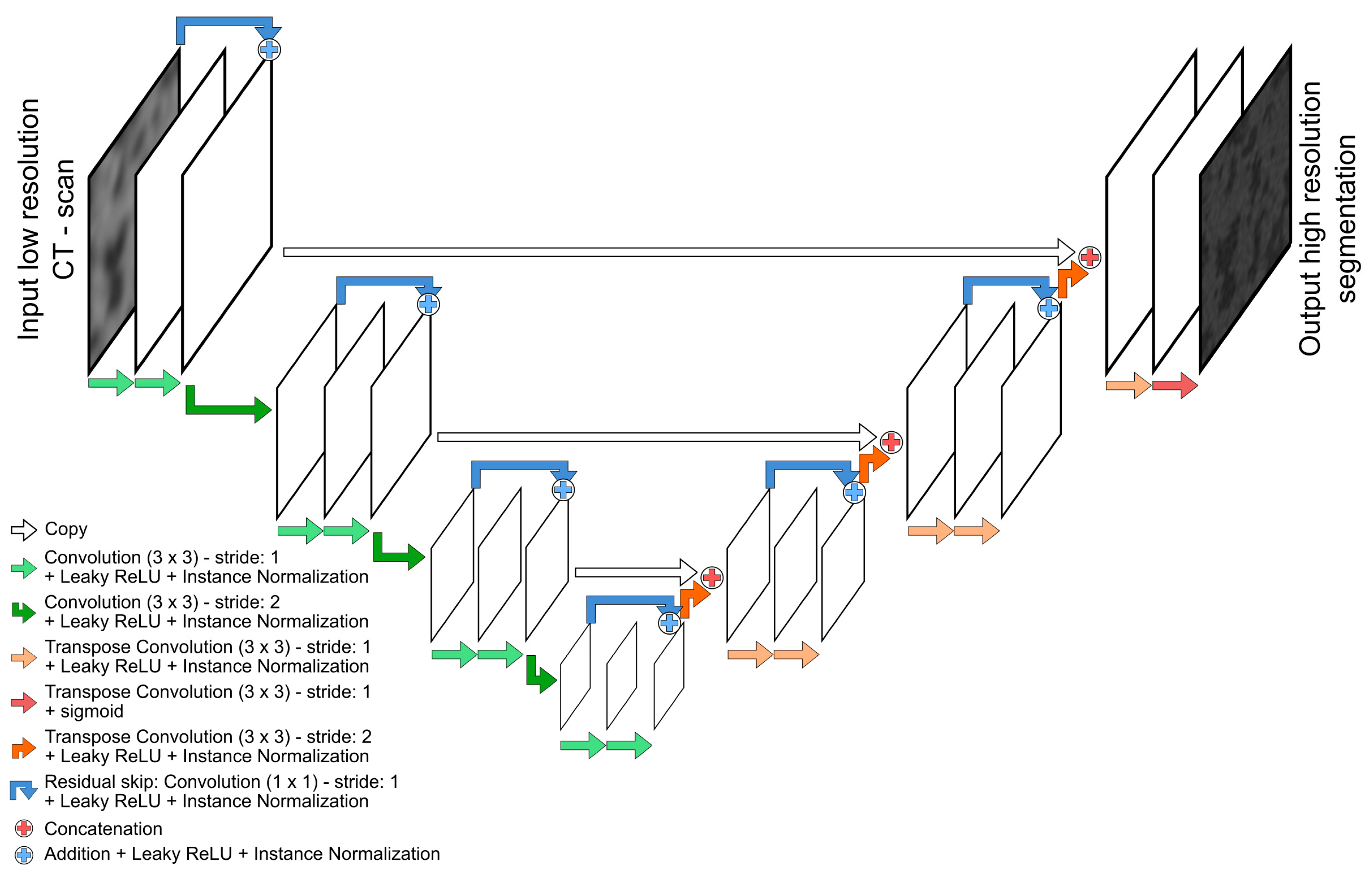
2.3.1. Convolutional Neural Network–Network Architecture
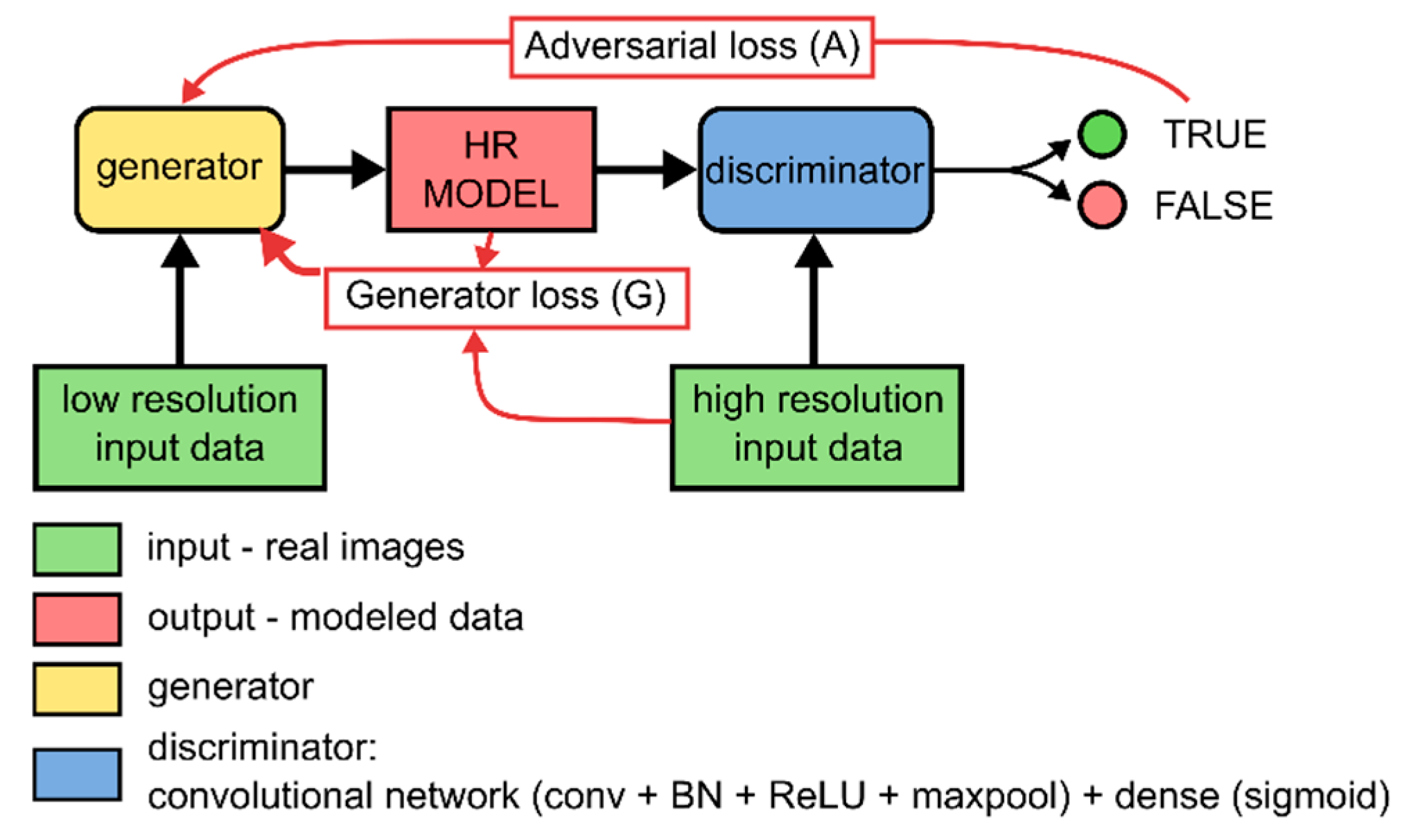
2.3.2. Conditional Generative Adversarial Networks (GAN)—Super-Resolution Images
2.3.3. Training
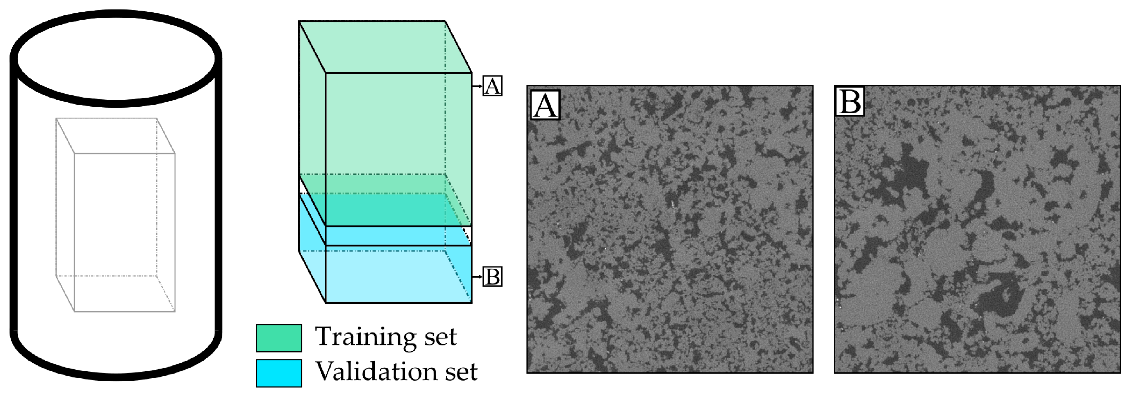
2.4. Dataset Preparation
2.5. Fluid Flow Properties
2.5.1. Lattice Boltzmann Simulation—Single-Phase Permeability
2.5.2. Pore Network Models (PNM)
2.5.3. Unsaturated Flow: Moisture
2.5.4. Two-Phase Flow: Oil and Water
3. Results
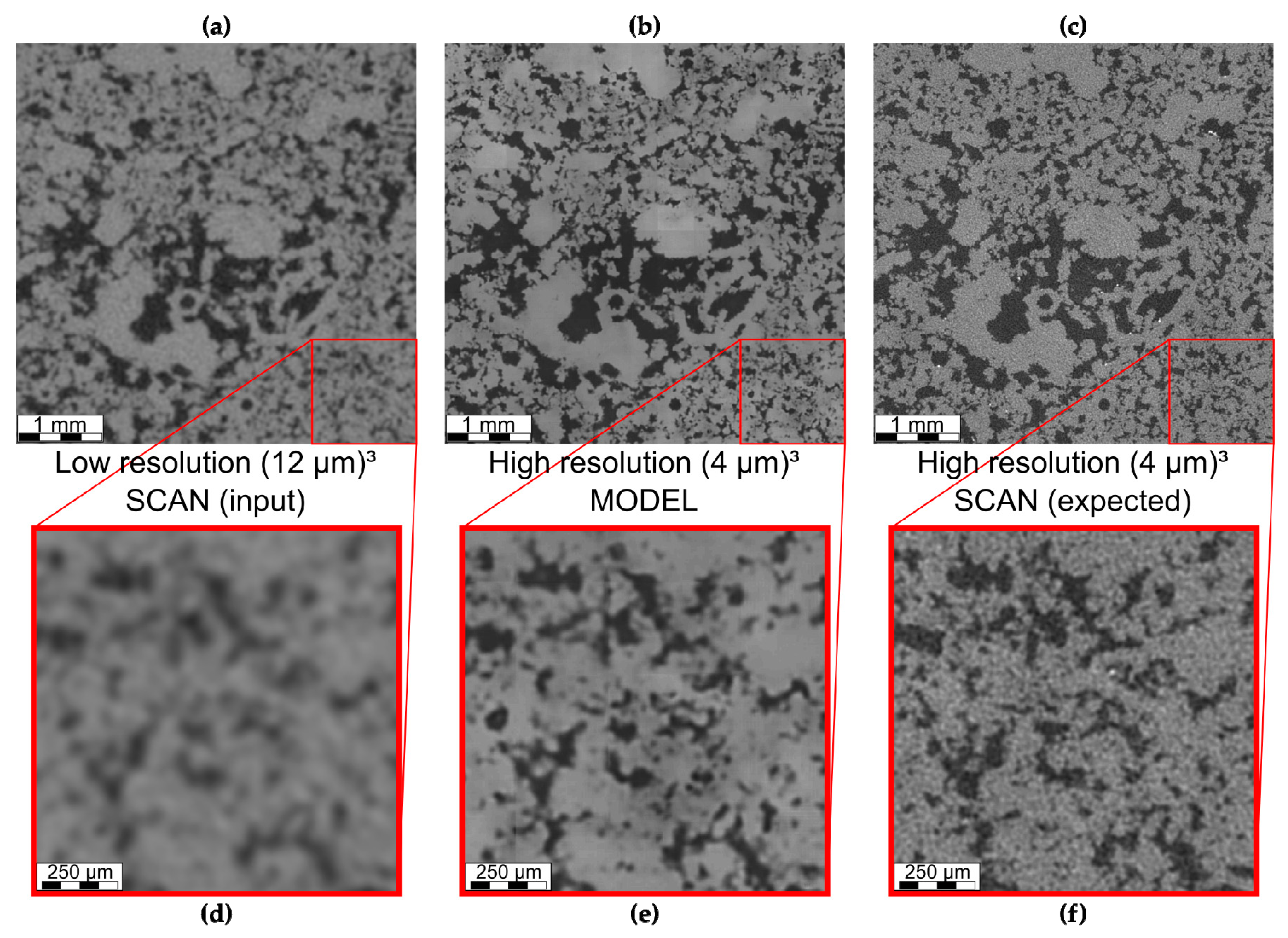
3.1. Visual Results
3.2. Pore Network Properties
3.3. Porosity and Absolute Permeability
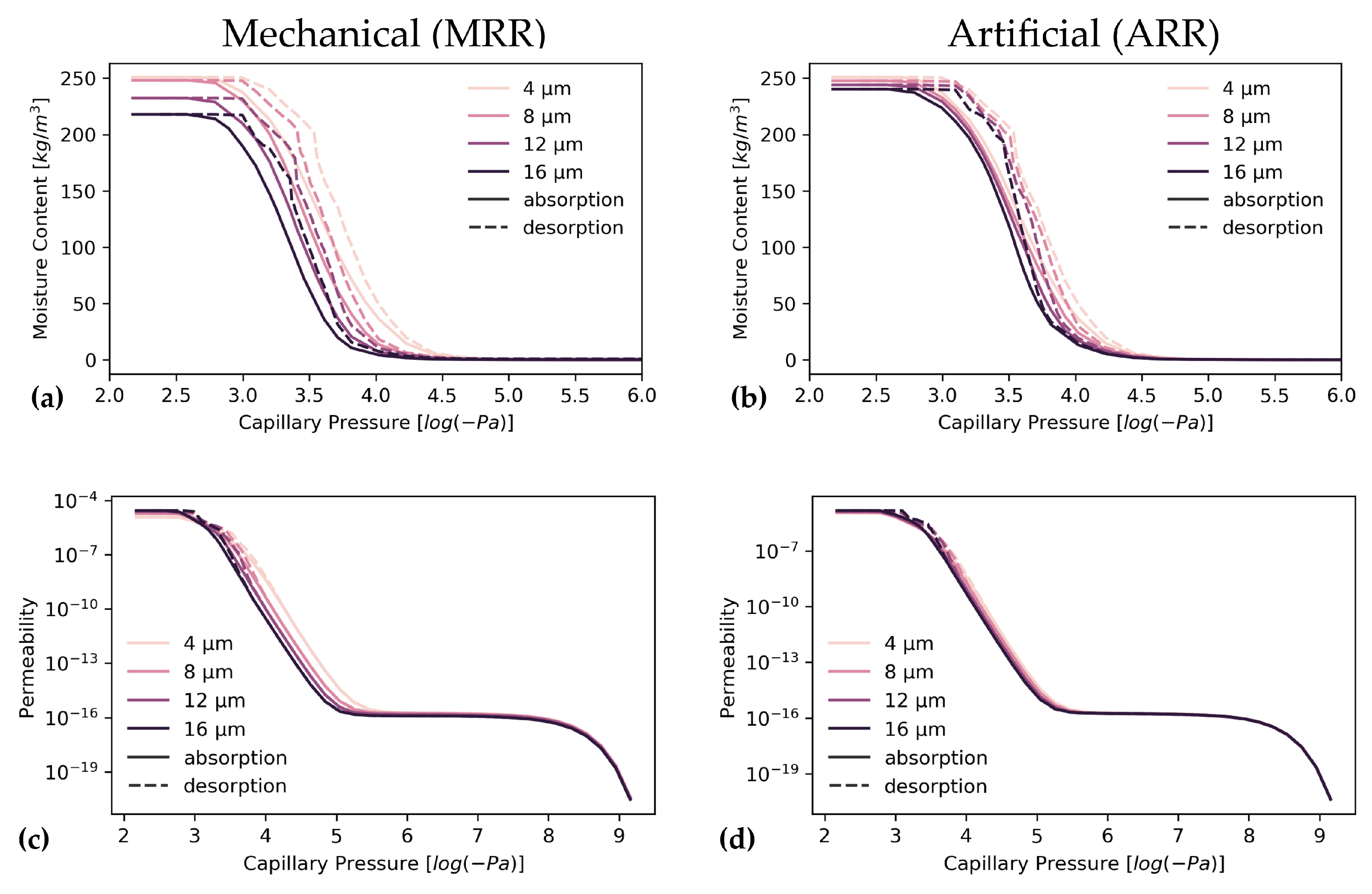
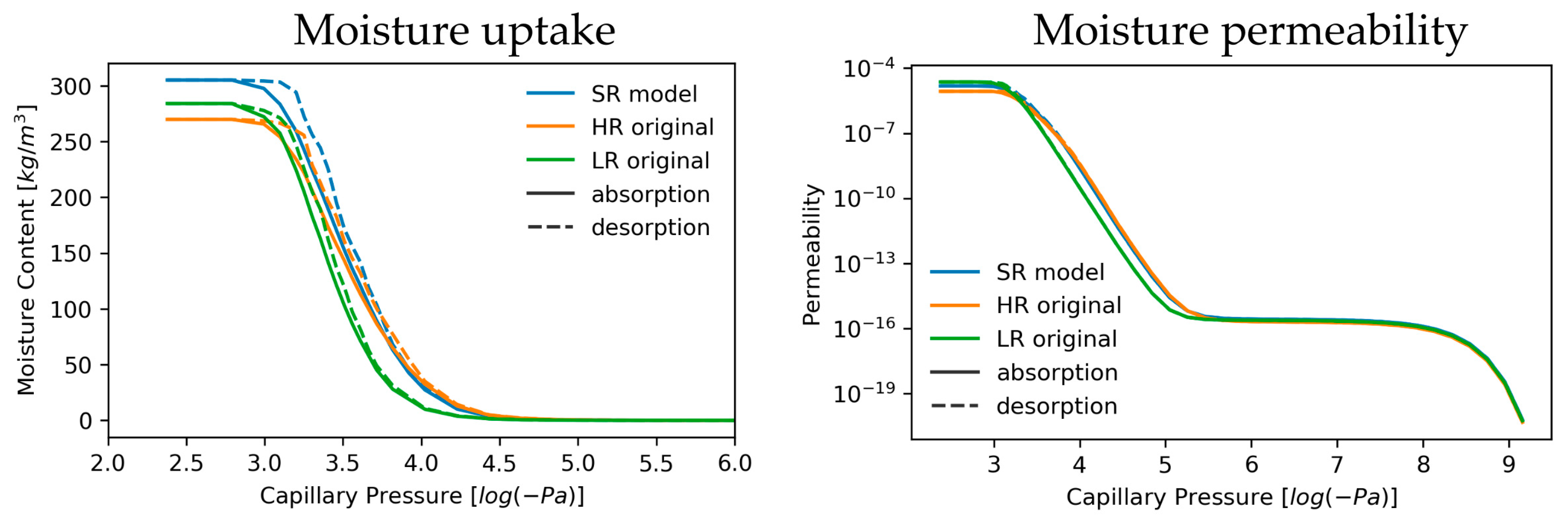
3.4. Unsaturated Flow
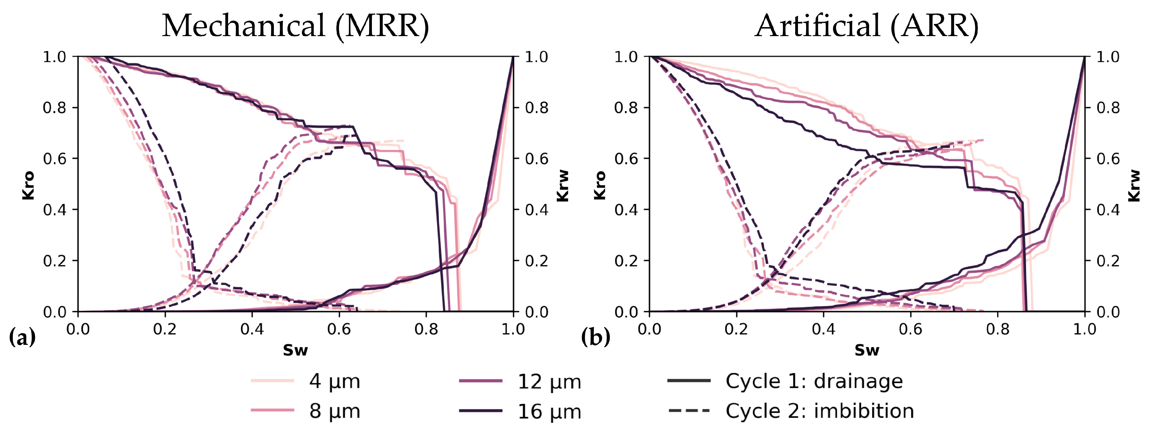
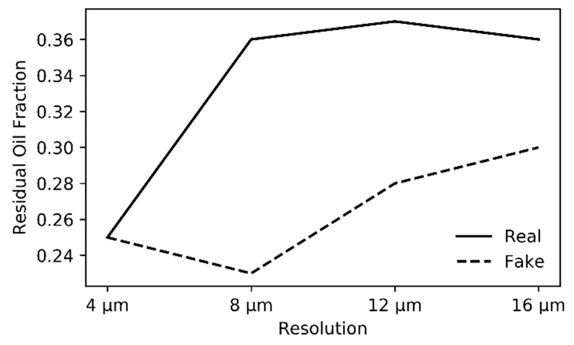
3.5. Two-Phase Flow
3.6. Training and Simulation Speed
4. Discussion
4.1. Resolution Influence
4.2. Super Resolution Models and Their Impact on Fluid Flow Simulation
4.3. Limitations and Future Perspectives
5. Conclusions
Supplementary Materials
Author Contributions
Funding
Acknowledgments
Conflicts of Interest
References
- Stappen, J.; Van de Kock, T.; Boone, M.A.; Olaussen, S.; Cnudde, V. Pore-scale characterisation and modelling of CO2flow in tight sandstones using X-ray micro-CT.; Knorringfjellet formation of the longyearbyen CO2lab, Svalbard. Nor. J. Geol. 2014, 94, 201–215. [Google Scholar]
- Andrew, M.; Menke, H.; Blunt, M.J.; Bijeljic, B. The Imaging of Dynamic Multiphase Fluid Flow Using Synchrotron-Based X-ray Microtomography at Reservoir Conditions. Transp. Porous Media 2015, 110, 1–24. [Google Scholar] [CrossRef]
- Menke, H.P.; Bijeljic, B.; Andrew, M.G.; Blunt, M.J. Dynamic three-dimensional pore-scale imaging of reaction in a carbonate at reservoir conditions. Environ. Sci. Technol. 2015, 49, 4407–4414. [Google Scholar] [CrossRef]
- Bachu, S. CO2 storage in geological media: Role, means, status and barriers to deployment. Prog. Energy Combust. Sci. 2008, 34, 254–273. [Google Scholar] [CrossRef]
- Metz, B.; Davidson, O.; de Coninck, H.; Loos, M.; Meyer, L. The IPCC Special Report on Carbon Dioxide Capture and Storage; Cambridge University Press: Cambridge, UK, 2005; ISBN 9608758424. [Google Scholar]
- Herzog, H.; Caldeira, K.; Reilly, J. An issue of permanence: Assessing the effectiveness of temporary carbon storage. Clim. Chang. 2003, 59, 293–310. [Google Scholar] [CrossRef]
- Valvatne, P.H.; Blunt, M.J. Predictive pore-scale modeling of two-phase flow in mixed wet media. Water Resour. Res. 2004, 40, 1–21. [Google Scholar] [CrossRef]
- Al-Kharusi, A.S.; Blunt, M.J. Multiphase flow predictions from carbonate pore space images using extracted network models. Water Resour. Res. 2008, 44, 1–14. [Google Scholar] [CrossRef]
- Blunt, M.J.; Bijeljic, B.; Dong, H.; Gharbi, O.; Iglauer, S.; Mostaghimi, P.; Paluszny, A.; Pentland, C. Pore-scale imaging and modelling. Adv. Water Resour. 2013, 51, 197–216. [Google Scholar] [CrossRef]
- Islahuddin, M.; Janssen, H. Hygric property estimation of porous building materials with multiscale pore structues. Energy Procedia 2017, 132, 273–278. [Google Scholar] [CrossRef]
- Janssen, H.; Vereecken, E.; Holúbek, M. A confrontation of two concepts for the description of the over-capillary moisture range: Air entrapment versus low capillarity. Energy Procedia 2015, 78, 1490–1494. [Google Scholar] [CrossRef]
- Roels, S.; Carmeliet, J.; Hens, H.; Adan, O.; Brocken, H.; Cerny, R.; Pavlik, Z.; Hall, C.; Kumaran, K.; Pel, L.; et al. Interlaboratory Comparison of Hygric Properties of Porous Building Materials. J. Therm. Envel. Build. Sci. 2004, 27, 307–325. [Google Scholar] [CrossRef]
- Arns, J.; Sheppard, A.P.; Arns, C.H.; Knackstedt, M.A.; Yelkhovsky, A.; Pinczewski, W.V. Pore-level validation of representative pore networks obtained from micro-CT images. In Proceedings of the Annual Symposium of the Society of Core Analysis, Calgary, Canada, 10–12 September 2007; p. 12. [Google Scholar]
- Knackstedt, M.; Jaime, P.; Butcher, A.R.; Botha, P.W.S.K.; Middleton, J.; Sok, R. Integrating reservoir characterization: 3D dynamic, petrophysical and geological description of reservoir facies. In Proceedings of the SPE Asia Pacific Oil & Gas Conference and Exhibition, Brisbane, Queensland, Australia, 18–20 October 2010; pp. 1–9. [Google Scholar]
- Hemes, S.; Desbois, G.; Urai, J.L.; De Craen, M.; Honty, M. Variations in the morphology of porosity in the Boom Clay Formation: Insights from 2D high resolution BIB-SEM imaging and Mercury injection Porosimetry. Neth. J. Geosci. 2013, 92, 275–300. [Google Scholar] [CrossRef]
- Keller, L.M.; Schuetz, P.; Erni, R.; Rossell, M.D.; Lucas, F.; Gasser, P.; Holzer, L. Characterization of multi-scale microstructural features in Opalinus Clay. Microporous Mesoporous Mater. 2013, 170, 83–94. [Google Scholar] [CrossRef]
- Janssen, H. Simulation efficiency and accuracy of different moisture transfer potentials. J. Build. Perform. Simul. 2014, 7, 379–389. [Google Scholar] [CrossRef]
- De Kock, T.; Boone, M.A.; De Schryver, T.; Van Stappen, J.; Derluyn, H.; Masschaele, B.; De Schutter, G.; Cnudde, V. A pore-scale study of fracture dynamics in rock using X-ray micro-CT under ambient freeze-thaw cycling. Environ. Sci. Technol. 2015, 49, 2867–2874. [Google Scholar] [CrossRef]
- Islahuddin, M.; Janssen, H. Pore-Structure-Based Determination of Unsaturated Hygric Properties of Porous Materials. Transp. Porous Media 2019, 130, 675–698. [Google Scholar] [CrossRef]
- Arns, C.; Bauget, F.; Sakellariou, A.; Senden, T.J.; Sheppard, A.P.; Sok, R.M.; Pinczewski, V.; Bakke, S.; Berge, L.I.; Oren, P.E.; et al. Pore Scale Characterization of Carbonates Using X-ray Microtomography. SPE J. 2005, 2005, 475–484. [Google Scholar] [CrossRef]
- Wildenschild, D.; Hopmans, J.W.; Rivers, M.L.; Kent, A.J.R. Quantitative analysis of flow processes in a sand using synchrotron-based X-ray microtomography. Vadose Zone J. 2005, 4, 112–126. [Google Scholar] [CrossRef]
- Wildenschild, D.; Sheppard, A.P. X-ray imaging and analysis techniques for quantifying pore-scale structure and processes in subsurface porous medium systems. Adv. Water Resour. 2013, 51, 217–246. [Google Scholar] [CrossRef]
- Bultreys, T.; Van Hoorebeke, L.; Cnudde, V. Multi-scale, micro-computed tomography-based pore network models to simulate drainage in heterogeneous rocks. Adv. Water Resour. 2015, 78, 36–49. [Google Scholar] [CrossRef]
- Cnudde, V.; Boone, M.N. High-resolution X-ray computed tomography in geosciences: A review of the current technology and applications. Earth Sci. Rev. 2013, 123, 1–17. [Google Scholar] [CrossRef]
- Ketcham, R.; Carlson, W.D. Acquisition, optimization and interpretation of x-ray computed tomographic imagery: Applications to the geosciences. Comput. Geosci. 2001, 27, 381–400. [Google Scholar] [CrossRef]
- Alyafei, N.; Raeini, A.Q.; Paluszny, A.; Blunt, M.J. A sensitivity study of the effect of image resolution on predicted petrophysical properties. Transp. Porous Media 2015, 110, 157–169. [Google Scholar] [CrossRef]
- Zhang, D.; Zhang, R.; Chen, S.; Soll, W.E. Pore scale study of flow in porous media: Scale dependency, REV, and statistical REV. Geophys. Res. Lett. 2000, 27, 1195–1198. [Google Scholar] [CrossRef]
- Bear, J.; Bachmat, Y. Introduction to Modeling of Transport Phenomena in Porous Media; Kluwer Academic Publishers: Dordrecht, The Netherlands, 1990; ISBN 0792305574. [Google Scholar]
- Thakur, M.M.; Penumadu, D.; Bauer, C. Capillary Suction Measurements in Granular Materials and Direct Numerical Simulations Using X-ray Computed Tomography Microstructure. J. Geotech. Geoenviron. Eng. 2020, 146, 1–13. [Google Scholar]
- Alyafei, N.; Gharbi, O.; Raeini, A.Q.; Yang, J.; Iglauer, S.; Blunt, M.J. Influence of micro-computed tomography image resolution on the predictions of petrophysical properties. In Proceedings of the Society of Petroleum Engineers-International Petroleum Technology Conference 2013, IPTC 2013: Challenging Technology and Economic Limits to Meet the Global Energy Demand, Beijing, China, 26–28 March 2013; pp. 1291–1298. [Google Scholar]
- Takbiri-Borujeni, A.; Lane, N.M.; Thompson, K.; Tyagi, M. Effects of image resolution and numerical resolution on computed permeability of consolidated packing using LB and FEM pore-scale simulations. Comput. Fluids 2013, 88, 753–763. [Google Scholar] [CrossRef]
- Shah, S.M.; Gray, F.; Crawshaw, J.P.; Boek, E.S. Micro-computed tomography pore-scale study of flow in porous media: Effect of voxel resolution. Adv. Water Resour. 2016, 95, 276–287. [Google Scholar] [CrossRef]
- Guan, K.M.; Nazarova, M.; Guo, B.; Tchelepi, H.; Kovscek, A.R.; Creux, P. Effects of image resolution on sandstone porosity and permeability as obtained from X-ray microscopy. Transp. Porous Media 2019, 127, 233–245. [Google Scholar] [CrossRef]
- Keehm, Y.; Mukerji, T. Permeability and relative permeability from digital rocks: Issues on grid resolution and representative elementary volume. In Proceedings of the SEG International Exposition and 74th Annual Meeting, Denver, CO, USA, 10–15 October 2004; pp. 1–3. [Google Scholar]
- Ortega Ramírez, M.P.; Oxarango, L.; Strozzi, A.G. Effect of X-ray CT resolution on the quality of permeability computation for granular soils: Definition of a criterion based on morphological properties. Soil Res. 2019, 57, 589–600. [Google Scholar] [CrossRef]
- Thakur, M.M.; Penumadu, D. Sensitivity analysis of pore morphology method and X-ray CT imaging in SWCC predictions for Ottawa Sand. In Advances in Computer Methods and Geomechanics. Lecture Notes in Civil Engineering; Prashant, A., Sachan, A., Desai, C., Eds.; Springer: Singapore, 2020. [Google Scholar]
- Bear, J. Dynamics of Fluids in Porous Media; American Elsevier: New York, NY, USA, 1972. [Google Scholar]
- Rozenbaum, O.; Du Roscoat, S.R. Representative elementary volume assessment of three-dimensional x-ray microtomography images of heterogeneous materials: Application to limestones. Phys. Rev. E Stat. Nonlinear Soft Matter Phys. 2014, 89, 1–11. [Google Scholar] [CrossRef]
- Mostaghimi, P.; Blunt, M.J.; Bijeljic, B. Computations of absolute permeability on micro-CT images. Math. Geosci. 2013, 45, 103–125. [Google Scholar] [CrossRef]
- Desbois, G.; Urai, J.L.; Hemes, S.; Schröppel, B.; Schwarz, J.O.; Mac, M.; Weiel, D. Multi-scale analysis of porosity in diagenetically altered reservoir sandstone from the Permian Rotliegend (Germany). J. Pet. Sci. Eng. 2016, 140, 128–148. [Google Scholar] [CrossRef]
- Sok, R.; Varslot, T.; Ghous, A.; Latham, S.; Sheppard, A.P.; Knackstedt, M.A. Pore scale characterization of carbonates at multiple scales: Integration of micro-CT, BSEM, and FIBSEM. Petrophysics 2010, 51, 379–387. [Google Scholar]
- Grader, A.S.; Clark, A.B.S.; Al-Dayyani, T.; Nur, A. Computations of porosity and permeability of sparic carbonate using multi-scale CT images. In Proceedings of the International Symposium of the Society of Core Analysts, Noordwijk aan Zee, The Netherlands, 27–30 September 2009; p. 10. [Google Scholar]
- Pamukcu, A.S.; Guilherme, A.R. Quantitative 3D petrography using X-ray tomography 2: Combining information at various resolutions. Geosphere 2010, 6, 775–781. [Google Scholar] [CrossRef]
- Prodanović, M.; Mehmani, A.; Sheppard, A.P. Imaged-based multiscale network modelling of microporosity in carbonates. Geol. Soc. Lond. Spec. Publ. 2014, 406, 95–113. [Google Scholar] [CrossRef]
- Tahmasebi, P.; Kamrava, S. Rapid multiscale modeling of flow in porous media. Phys. Rev. E 2018, 98, 1–13. [Google Scholar] [CrossRef]
- Mehmani, A.; Prodanović, M. The effect of microporosity on transport properties in porous media. Adv. Water Resour. 2014, 63, 104–119. [Google Scholar] [CrossRef]
- Jiang, Z.; Van Dijke, M.I.J.; Sorbie, K.S.; Couples, G.D. Representation of multiscale heterogeneity via multiscale pore networks. Water Resour. Res. 2013, 49, 5437–5449. [Google Scholar] [CrossRef]
- Yao, J.; Wang, C.; Yang, Y.; Wang, X. Upscaling of carbonate rocks from micropore scale to core scale. Int. J. Multiscale Comput. Eng. 2013, 11, 497–504. [Google Scholar] [CrossRef]
- Moctezuma, A.; Békri, S.; Laroche, C.; Vizika, O. A Dual Network Model for Relative Permeability of Bimodal Rocks: Application in a Vuggy Carbonate. In Proceedings of the International Symposium of the Society of Core Analysts, Pau, France, 21–24 September 2003; pp. 1–13. [Google Scholar]
- Békri, S.; Laroche, C.; Vizika, O. Pore Network Models To Calculate Transport and Electrical Properties of Single or Dual-Porosity Rocks. In Proceedings of the International Symposium of the Society of Core Analysts, Toronto, Canada, 21–25 August 2005; pp. 1–16. [Google Scholar]
- Youssef, S.; Rosenberg, E.; Gland, N.; Kenter, J.A.M.; Skalinski, M.; Vizika, O. High resolution CT and pore-network models to assess petrophysical properties of homogeneous and heterogeneous carbonates. In Proceedings of the SPE/EAGE Reservoir Characterization and Simulation Conference, Abu Dhabi, UAE, 28–31 October 2007; pp. 280–291. [Google Scholar]
- Bauer, D.; Youssef, S.; Fleury, M.; Bekri, S.; Rosenberg, E.; Vizika, O. Improving the estimations of petrophysical transport behavior of carbonate rocks using a dual pore network approach combined with computed microtomography. Transp. Porous Media 2012, 94, 505–524. [Google Scholar] [CrossRef]
- De Vries, E.T.; Raoof, A.; Van Genuchten, M. Advances in Water Resources Multiscale modelling of dual-porosity porous media; A computational pore-scale study for flow and solute transport. Adv. Water Resour. 2017, 105, 82–95. [Google Scholar] [CrossRef]
- Dong, H.; Blunt, M.J. Pore-network extraction from micro-computerized-tomography images. Phys. Rev. E 2009, 80, 036307. [Google Scholar] [CrossRef] [PubMed]
- Raeini, A.Q.; Bijeljic, B.; Blunt, M.J. Generalized network modeling: Network extraction as a coarse-scale discretization of the void space of porous media. Phys. Rev. E 2017, 96, 1–17. [Google Scholar] [CrossRef] [PubMed]
- Øren, P.E.; Bakke, S.; Arntzen, O.J. Extending Predictive Capabilities to Network Models. SPE J. 1998, 3, 324–335. [Google Scholar] [CrossRef]
- Wu, K.; Nunan, N.; Crawford, J.W.; Young, I.M.; Ritz, K. An efficient Markov Chain Model for the Simulation of Heterogeneous Soil Structure. Soil Sci. Soc. Am. J. 2004, 68, 346–351. [Google Scholar] [CrossRef]
- Gerke, K.M.; Karsanina, M.V.; Mallants, D. Universal stochastic multiscale image fusion: An example application for shale rock. Sci. Rep. 2015, 5, 1–12. [Google Scholar] [CrossRef]
- Yao, J.; Wang, C.; Yang, Y.; Hu, R.; Wang, X. The construction of carbonate digital rock with hybrid superposition method. J. Pet. Sci. Eng. 2013, 110, 263–267. [Google Scholar] [CrossRef]
- Karsanina, M.V.; Gerke, K.M.; Skvortsova, E.B.; Ivanov, A.L.; Mallants, D. Enhancing image resolution of soils by stochastic multiscale image fusion. Geoderma 2018, 314, 138–145. [Google Scholar] [CrossRef]
- Karsanina, M.V.; Gerke, K.M. Hierarchical optimization: Fast and robust multiscale stochastic reconstructions with rescaled correlation functions. Phys. Rev. Lett. 2018, 121, 1–6. [Google Scholar] [CrossRef]
- Bakke, S.; Øren, P.-E. 3-D Pore-Scale Modelling of Sandstones and Flow Simulations in the Pore Networks. SPE J. 1997, 2, 136–149. [Google Scholar] [CrossRef]
- Quiblier, J.A. A new three-dimensional modeling technique for studying porous media. J. Colloid Interface Sci. 1984, 98, 84–102. [Google Scholar] [CrossRef]
- Caers, J. A General Algorithm for Building 3D Spatial Laws from Lower Dimensional Structural Information; Stanford University: Main Quad, CA, USA, 2006. [Google Scholar]
- Jiao, Y.; Stillinger, F.H.; Torquato, S. Modeling heterogeneous materials via two-point correlation functions. II. Algorithmic details and applications. Phys. Rev. E Stat. Nonlinear Soft Matter Phys. 2008, 77, 1–35. [Google Scholar] [CrossRef] [PubMed]
- Hasanabadi, A.; Baniassadi, M.; Abrinia, K.; Safdari, M.; Garmestani, H. 3D microstructural reconstruction of heterogeneous materials from 2D cross sections: A modified phase-recovery algorithm. Comput. Mater. Sci. 2016, 111, 107–115. [Google Scholar] [CrossRef]
- Izadi, H.; Baniassadi, M.; Hormozzade, F.; Dehnavi, F.N.; Hasanabadi, A.; Memarian, H.; Soltanian-Zadeh, H. Effect of 2D Image Resolution on 3D Stochastic Reconstruction and Developing Petrophysical Trend. Transp. Porous Media 2018, 125, 41–58. [Google Scholar] [CrossRef]
- Okabe, H.; Blunt, M.J. Pore space reconstruction using multiple-point statistics. J. Pet. Sci. Eng. 2005, 46, 121–137. [Google Scholar] [CrossRef]
- Hajizadeh, A.; Safekordi, A.; Farhadpour, F. A multiple-point statistics algorithm for 3D pore space reconstruction from 2D images. Adv. Water Resour. 2011, 34, 1256–1267. [Google Scholar] [CrossRef]
- Ding, K.; Teng, Q.; Wang, Z.; He, X.; Feng, J. Improved multipoint statistics method for reconstructing three-dimensional porous media from a two-dimensional image via porosity matching. Phys. Rev. E 2018, 97, 1–10. [Google Scholar] [CrossRef]
- Comunian, A.; Renard, P.; Straubhaar, J. 3D multiple-point statistics simulation using 2D training images. Comput. Geosci. 2012, 40, 49–65. [Google Scholar] [CrossRef]
- Soete, J.; Claes, S.; Claes, H.; Janssens, N.; Cnudde, V.; Huysmans, M.; Swennen, R. Lattice Boltzmann Simulations of fluid flow in continental carbonate reservoir rocks and in upscaled rock models generated with multiple-point geostatistics. Geofluids 2017, 1–24. [Google Scholar] [CrossRef]
- Okabe, H.; Blunt, M.J. Pore space reconstruction of vuggy carbonates using microtomography and multiple-point statistics. Water Resour. Res. 2007, 43, 3–7. [Google Scholar] [CrossRef]
- Tahmasebi, P.; Javadpour, F.; Sahimi, M.; Piri, M. Multiscale study for stochastic characterization of shale samples. Adv. Water Resour. 2016, 89, 91–103. [Google Scholar] [CrossRef]
- Wu, Y.; Tahmasebi, P.; Lin, C.; Ren, L.; Dong, C. Multiscale modeling of shale samples based on low- and high-resolution images. Mar. Pet. Geol. 2019, 109, 9–21. [Google Scholar] [CrossRef]
- Lemmens, L.; Rogiers, B.; Jacques, D.; Huysmans, M.; Swennen, R.; Urai, J.L.; Desbois, G.; Laloy, E. Nested multiresolution hierarchical simulated annealing algorithm for porous media reconstruction. Phys. Rev. E 2019, 100, 1–21. [Google Scholar] [CrossRef] [PubMed]
- Campaigne, W.R.; Fieguth, P.W. Frozen-State Hierarchical Annealing. IEEE Trans. Image Process. 2013, 22, 1486–1497. [Google Scholar] [CrossRef] [PubMed]
- Pant, L.M.; Berkeley, L.; Secanell, M. Multigrid hierarchical simulated annealing method for reconstructing heterogeneous media A Multigrid Hierarchical Simulated Annealing Method for Reconstructing. Phys. Rev. E 2015, 92, 1–12. [Google Scholar] [CrossRef] [PubMed]
- Mariethoz, G.; Renard, P.; Straubhaar, J. Extrapolating the fractal characteristics of an image using scale-invariant multiple-point statistics. Math. Geosci. 2011, 43, 783–797. [Google Scholar] [CrossRef][Green Version]
- Plenge, E.; Poot, D.H.J.; Niessen, W.J.; Meijering, E. Super-Resolution reconstruction using cross-scale self-similarity in multi-slice MRI. In Proceedings of the Medical Image Computing and Computer-Assisted Intervention-MICCAI, Nagoya, Japan, 22–26 September 2013; Springer: Berlin/Heidelberg, Germany, 2013; pp. 123–130. [Google Scholar]
- Glasner, D.; Bagon, S.; Irani, M. Super-Resolution from a Single Image. In Proceedings of the 2009 IEEE 12th International Conference on Computer Vision, Kyoto, Japan, 29 September–2 October 2009; pp. 349–356. [Google Scholar]
- Wang, Y.; Rahman, S.S.; Arns, C.H. Super resolution reconstruction of µ -CT image of rock sample using neighbour embedding algorithm. Physica A 2018, 493, 177–188. [Google Scholar] [CrossRef]
- Wang, Y.; Arns, J.Y.; Rahman, S.S.; Arns, C.H. Three-dimensional porous structure reconstruction based on structural local similarity via sparse representation on micro-computed-tomography images. Phys. Rev. E 2018, 98, 1–16. [Google Scholar] [CrossRef]
- Wang, Y.; Arns, C.H.; Rahman, S.S.; Arns, J. Porous structure reconstruction using convolutional neural networks. Math. Geosci. 2018, 50, 781–799. [Google Scholar] [CrossRef]
- Wang, Y.; Teng, Q.; He, X.; Feng, J.; Zhang, T. CT-image of rock samples super resolution using 3D convolutional neural network. Comput. Geosci. 2019, 133, 1–11. [Google Scholar] [CrossRef]
- Dong, C.; Loy, C.C.; He, K.; Tang, X. Image Super-Resolution Using Deep Convolutional Networks. IEEE Trans. Pattern Anal. Mach. Intell. 2016, 38, 295–307. [Google Scholar] [CrossRef] [PubMed]
- Ledig, C.; Theis, L.; Huszár, F.; Caballero, J.; Cunningham, A.; Acosta, A.; Aitken, A.; Tejani, A.; Totz, J.; Wang, Z.; et al. Photo-realistic single image super-resolution using a generative adversarial network. In Proceedings of the 30th IEEE Conference on Computer Vision and Pattern Recognition, Honolulu, HI, USA, 21–26 July 2017; pp. 105–114. [Google Scholar]
- Shams, R.; Masihi, M.; Boozarjomehry, R.B.; Blunt, M.J. Coupled generative adversarial and auto-encoder neural networks to reconstruct three-dimensional multi-scale porous media. J. Pet. Sci. Eng. 2020, 186, 1–15. [Google Scholar] [CrossRef]
- Latief, F.D.E.; Fauzi, U.; Irayani, Z.; Dougherty, G. The effect of X-ray micro computed tomography image resolution on flow properties of porous rocks. J. Microsc. 2017, 266, 69–88. [Google Scholar] [CrossRef]
- Fukushima, K. Neocognitron: A self-organizing neural network model for a mechanism of pattern recognition unaffected by shift in position. Biol. Cybermetics 1980, 36, 193–202. [Google Scholar] [CrossRef] [PubMed]
- Weng, J.J.; Ahuja, N.; Huang, T.S. Learning recognition and segmentation of 3-D objects from 2-D images. In Proceedings of the 1993 IEEE 4th International Conference on Computer Vision, Berlin, Germany, 11–14 May 1993; pp. 121–127. [Google Scholar]
- Lecun, Y.; Bengio, Y.; Hinton, G. Deep learning. Nature 2015, 521, 436–444. [Google Scholar] [CrossRef] [PubMed]
- Dong, C.; Loy, C.C.; He, K.; Tang, X. Learning a deep convolutional network for image super-resolution. In Proceedings of the Lecture Notes in Computer Science, Zurich, Switzerland, 6–12 September 2014; Fleet, D., Pajdla, T., Schiele, B., Tuytelaars, T., Eds.; Springer: Cham, Switzerland, 2014; Volume 8692, pp. 184–199. [Google Scholar]
- Dong, C.; Loy, C.C.; Tang, X. Accelerating the super-resolution convolutional neural network. In Proceedings of the Lecture Notes in Computer Science, Amsterdam, The Netherlands, 11–14 October 2016; Volume 9906, pp. 391–407. [Google Scholar]
- Kim, J.; Lee, J.K.; Lee, K.M. Accurate Image Super-Resolution Using Very Deep Convolutional Networks. In Proceedings of the 2016 IEEE Conference on Computer Vision and Pattern Recognition (CVPR), Las Vegas Valley, NV, USA, 26 June–1 July 2016; pp. 1646–1654. [Google Scholar]
- Mao, X.J.; Shen, C.; Yang, B.Y. Image restoration using very deep convolutional encoder-decoder networks with symmetric skip connections. In Proceedings of the Advances in Neural Information Processing Systems, Barcelona, Spain, 5–10 December 2016; pp. 2810–2818. [Google Scholar]
- Kupyn, O.; Budzan, V.; Mykhailych, M.; Mishkin, D.; Matas, J. DeblurGAN: Blind Motion Deblurring Using Conditional Adversarial Networks. In Proceedings of the IEEE Computer Society Conference on Computer Vision and Pattern Recognition, Salt Lake City, UT, USA, 18–22 June 2018; pp. 8183–8192. [Google Scholar]
- Chang, Y.; Luo, B. Bidirectional convolutional LSTM neural network for remote sensing image super-resolution. Remote Sens. 2019, 11, 1–18. [Google Scholar] [CrossRef]
- Liebel, L.; Körner, M. Single-image super resolution for multispectral remote sensing data using convolutional neural networks. In Proceedings of the International Archives of the Photogrammetry, Remote Sensing and Spatial Information Sciences-ISPRS Archives, Prague, Czech Republic, 12–19 July 2016; Volume 41, pp. 883–890. [Google Scholar]
- Kaji, S.; Kida, S. Overview of image-to-image translation by use of deep neural networks: Denoising, super-resolution, modality conversion, and reconstruction in medical imaging. Radiol. Phys. Technol. 2019, 12, 235–248. [Google Scholar] [CrossRef]
- Chen, Y.; Shi, F.; Christodoulou, A.G.; Xie, Y.; Zhou, Z.; Li, D. Efficient and accurate MRI super-resolution using a generative adversarial network and 3D multi-level densely connected network. In Proceedings of the Lecture Notes in Computer Science, Grenada, Spain, 16–20 September 2018; Frangi, A., Schnabel, J., Davatzikos, C., Alberola-López, C.F.G., Eds.; Springer: Cham, Switzerland, 2018; Volume 11070, pp. 91–99. [Google Scholar]
- Pham, C.H.; Tor-Díez, C.; Meunier, H.; Bednarek, N.; Fablet, R.; Passat, N.; Rousseau, F. Multiscale brain MRI super-resolution using deep 3D convolutional networks. Comput. Med. Imaging Graph. 2019, 77, 1–15. [Google Scholar] [CrossRef]
- Umehara, K.; Ota, J.; Ishimaru, N.; Ohno, S.; Okamoto, K.; Suzuki, T.; Shirai, N.; Ishida, T. Super-resolution convolutional neural network for the improvement of the image quality of magnified images in chest radiographs. In Proceedings of the Medical Imaging 2017, Orlando, FL, USA, 13–16 February 2017; Image Processing. Styner, M.A., Angelini, E.D., Eds.; International Society for Optics and Photonics: Washington, DC, USA, 2017; Volume 10133, pp. 1–8. [Google Scholar]
- Umehara, K.; Ota, J.; Ishida, T. Application of Super-Resolution convolutional neural network for enhancing image resolution in chest CT. J. Digit. Imaging 2018, 31, 441–450. [Google Scholar] [CrossRef]
- Hatvani, J.; Horvath, A.; Michetti, J.; Basarab, A.; Kouame, D.; Gyongy, M. Deep Learning-Based Super-Resolution Applied to Dental Computed Tomography. IEEE Trans. Radiat. Plasma Med. Sci. 2019, 3, 120–128. [Google Scholar] [CrossRef]
- Li, M.; Shen, S.; Gao, W.; Hsu, W.; Cong, J. Computed tomography image enhancement using 3D convolutional neural network. In Proceedings of the Lecture Notes in Computer Science, Grenada, Spain, 20 September 2018; pp. 291–299. [Google Scholar]
- You, C.; Li, G.; Zhang, Y.; Zhang, X.; Shan, H.; Li, M.; Ju, S.; Zhao, Z.; Zhang, Z.; Cong, W.; et al. CT Super-resolution GAN Constrained by the Identical, Residual, and Cycle Learning Ensemble (GAN-CIRCLE). IEEE Trans. Med. Imaging 2019, 39, 188–203. [Google Scholar] [CrossRef]
- Goodfellow, I.J.; Pouget-Abadie, J.; Mirza, M.; Xu, B.; Warde-farley, D.; Ozair, S.; Courville, A.; Bengio, Y. Generative Adversarial Nets. In Proceedings of the NIPS’14 27th International Conference on Neural Information Processing Systems, Montréal, QC, Canada, 8–13 December 2014; pp. 2672–2680. [Google Scholar]
- Zhang, H.; Xu, T.; Li, H.; Zhang, S.; Wang, X.; Huang, X.; Metaxas, D.N. StackGAN++: Realistic Image Synthesis with Stacked Generative Adversarial Networks. IEEE Trans. Pattern Anal. Mach. Intell. 2016, 1–14. [Google Scholar]
- Mosser, L.; Dubrule, O.; Blunt, M.J. Stochastic Reconstruction of an Oolitic Limestone by Generative Adversarial Networks. Transp. Porous Media 2018, 125, 81–103. [Google Scholar] [CrossRef]
- Mosser, L.; Dubrule, O.; Blunt, M.J. Reconstruction of three-dimensional porous media using generative adversarial neural networks. Phys. Rev. E 2017, 96, 1–17. [Google Scholar] [CrossRef]
- Mosser, L.; Dubrule, O.; Blunt, M.J. Conditioning of generative adversarial networks for pore and reservoir scale models. In Proceedings of the 80th EAGE Conference and Exhibition 2018: Opportunities Presented by the Energy Transition, Copenhagen, Denmark, 11–14 June 2018; pp. 1–5. [Google Scholar]
- Pedley, M. Tufas and travertines of the Mediterranean region: A testing ground for freshwater carbonate concepts and developments. Sedimentology 2009, 56, 221–246. [Google Scholar] [CrossRef]
- Claes, H.; Soete, J.; Van Noten, K.; El Desouky, H.; Marques Erthal, M.; Vanhaecke, F.; Özkul, M.; Swennen, R. Sedimentology, three-dimensional geobody reconstruction and carbon dioxide origin of Pleistocene travertine deposits in the Ballık area (south-west Turkey). Sedimentology 2015, 62, 1408–1445. [Google Scholar] [CrossRef]
- Ronchi, P.; Cruciani, F. Continental carbonates as hydrocarbon reservoir, an analog case study from the travertine of Saturnia, Italy. Am. Assoc. Pet. Geol. Bull. 2015, 99, 711–734. [Google Scholar] [CrossRef]
- Mancini, A.; Capezzuoli, E.; Erthal, M.; Swennen, R. Hierarchical approach to define travertine depositional systems: 3D conceptual morphological model and possible applications. Mar. Pet. Geol. 2019, 103, 549–563. [Google Scholar] [CrossRef]
- Terra, J.G.S.; Spadini, A.R.; França, A.B.; Sombra, C.L.; Zambonato, E.E.; Juschaks, L.C.S.; Arienti, L.M.; Erthal, M.M.; Blauth, M.; Franco, M.P.; et al. Classificações clássicas de rochas carbonáticas. Bol. Geociencas Petrobras 2010, 18, 9–29. [Google Scholar]
- Borsato, R.; Jones, W.; Greenhalgh, J.; Martin, M.; Roberson, R. South Atlantic Conjugate Margin: An Exploration Strategy. First Break 2012, 30, 79–84. [Google Scholar]
- Lottaroli, F.; Meciani, L.; Andreotti, P. West Africa Presalt Exploration: Background and Perspective of the West African “Tupi” myth. In Proceedings of the New Understanding of the Petroleum Systems of Continental Margins of the World, Houston, TX, USA, 2–5 December 2012; pp. 460–468. [Google Scholar]
- Soete, J.; Claes, S.; Claes, H.; Erthal, M.M.; De Boever, E.; Foubert, A.; Klitzsch, N.; Özkul, M.; Swennen, R. Unravelling the pore network and its behaviour: An integrated NMR, MIP and petrographical study of continental carbonates from the Ballık area, SW Turkey. Mar. Pet. Geol. 2016, 59, 320–335. [Google Scholar] [CrossRef]
- Soete, J.; Kleipool, L.M.; Claes, H.; Claes, S.; Hamaekers, H.; Kele, S.; Özkul, M.; Foubert, A.; Reijmer, J.J.G.; Swennen, R. Acoustic properties in continental carbonates and their relation to depositional environments, porosity and pore types. Mar. Pet. Geol. 2015, 59, 320–335. [Google Scholar] [CrossRef]
- Wirjadi, O. Survey of 3D image segmentation methods. Ber. Fraunhofer ITWM 2007, 123, 1–25. [Google Scholar]
- Canny, J. A computational approach to edge detection. IEEE Trans. Pattern Anal. Mach. Intell. 1986, 8, 679–698. [Google Scholar] [CrossRef] [PubMed]
- Ronneberger, O.; Fischer, P.; Brox, T. U-net: Convolutional networks for biomedical image segmentation. In Proceedings of the Lecture Notes in Computer Science, Munich, Germany, 5–9 October 2015; Volume 9351, pp. 234–241. [Google Scholar]
- Maas, A.L.; Hannun, A.Y.; Ng, A.Y. Rectifier nonlinearities improve neural network acoustic models. In Proceedings of the ICML Workshop on Deep Learning for Audio, Speech and Language Processing, Atlanta, Georgia, 16 June 2013; Volume 28, pp. 1–6. [Google Scholar]
- Ulyanov, D.; Vedaldi, A.; Lempitsky, V. Improved texture networks: Maximizing quality and diversity in feed-forward stylization and texture synthesis. In Proceedings of the 30th IEEE Conference on Computer Vision and Pattern Recognition, Honolulu, HI, USA, 21–26 July 2017; pp. 4105–4113. [Google Scholar]
- Drozdzal, M.; Vorontsov, E.; Chartrand, G.; Kadoury, S.; Pal, C. The importance of skip connections in biomedical image segmentation. In Proceedings of the Lecture Notes in Computer Science, Athens, Greece, 17–21 October 2016; Volume 10008, pp. 179–187. [Google Scholar]
- Lim, B.; Son, S.; Kim, H.; Nah, S.; Lee, K.M. Enhanced Deep Residual Networks for Single Image Super-Resolution. In Proceedings of the IEEE Computer Society Conference on Computer Vision and Pattern Recognition Workshops, Honolulu, HI, USA, 21–26 July 2017; pp. 1132–1140. [Google Scholar]
- He, K.; Zhang, X.; Ren, S.; Sin, J. Deep Residual Learning for Image Recognition. In Proceedings of the IEEE Conference on Computer Vision and Pattern Recognition, Las Vegas, NV, USA, 26 June–1 July 2016; pp. 1951–1954. [Google Scholar]
- Radford, A.; Metz, L.; Chintala, S. Unsupervised representation learning with deep convolutional generative adversarial networks. arXiv 2015, arXiv:1511.06434. [Google Scholar]
- Salimans, T.; Goodfellow, I.; Cheung, V.; Radford, A.; Chen, X. Improved Techniques for Training GANs. arXiv 2016, arXiv:1606.03498. [Google Scholar]
- Mirza, M.; Osindero, S. Conditional Generative Adversarial Nets. arXiv 2014, arXiv:1411.1784. [Google Scholar]
- Mirsky, Y.; Mahler, T.; Shelef, I.; Elovici, Y. CT-GAN: Malicious Tampering of 3D medical imagery using deep learning. In Proceedings of the 28th USENIX Security Symposium, Santa Clara, CA, USA, 14–16 August 2019; pp. 461–478. [Google Scholar]
- Wang, Z.; Bovik, A.C.; Sheikh, H.R.; Simoncelli, E.P. Image quality assessment: From error visibility to structural similarity. IEEE Trans. Image Process. 2004, 13, 600–612. [Google Scholar] [CrossRef]
- Sukop, M.C.; Thorne, D.T. Lattice Boltzmann Modeling: An Introduction for Geoscientists and Engineers; Springer: Berlin, Germany, 2006; ISBN 9783540279815. [Google Scholar]
- Bhatnagar, P.L.; Gross, E.P.; Krook, M. A model for collision processes in gases. I. Small amplitude processes in charged and neutral one-component systems. Phys. Rev. 1954, 94, 511–525. [Google Scholar] [CrossRef]
- Succi, S. The Lattice Boltzmann Equation for Fluid Dynamics and Beyond; Clarendon Press: Oxford, UK, 2001. [Google Scholar]
- Meakin, P.; Tartakovsky, A.M. Modeling and simulation of pore-scale multiphase fluid flow and reactive transport in fractured and porous media. Rev. Geophys. 2009, 47, 1–47. [Google Scholar] [CrossRef]
- Mei, R.; Shyy, W.; Yu, D.; Luo, L.S. Lattice Boltzmann Method for 3-D Flows with Curved Boundary. J. Comput. Phys. 2000, 161, 680–699. [Google Scholar] [CrossRef]
- Latt, J. alabos: Parallel lattice Boltzmann solver, FlowKit-Numeca; Unige Palabos: Lausanne, Switzerland, 2009. [Google Scholar]
- Ahrens, J.; Geveci, B.; Law, C. ParaView: An End-User Tool for Large Data Visualization. In The Visualization Handbook; Elsevier: Amsterdam, The Netherlands, 2005. [Google Scholar]
- Ayachit, U. The ParaView Guide: A Parallel Visualization Application; Kitware: Clifton Park, NY, USA, 2015. [Google Scholar]
- Islahuddin, M.; Janssen, H. Numerical estimation of isothermal moisture storage and transport properties. In Proceedings of the Central European Symposium on Building Physics, Dresden, Germany, 14–16 September 2016; pp. 301–308. [Google Scholar]
- Gostick, J.; Aghighi, M.; Hinebaugh, J.; Tranter, T.; Hoeh, M.A.; Day, H.; Spellacy, B.; Sharqawy, M.H.; Bazylak, A.; Burns, A.; et al. OpenPNM: A Pore Network Modeling Package. Comput. Sci. Eng. 2016, 18, 60–74. [Google Scholar] [CrossRef]
- Valvatne, P.H. Predictive Pore-Scale Modelling of Multiphase Flow; Imperial College London: London, UK, 2004. [Google Scholar]
- Lenormand, R.; Zarcone, C.; Sarr, A. Mechanisms of the displacement of one fluid by another in a network of capillary ducts. J. Fluid Mech. 1983, 135, 337–353. [Google Scholar] [CrossRef]
- Mason, G.; Morrow, N.R. Capillary behavior of a perfectly wetting liquid in irregular triangular tubes. J. Colloid Interface Sci. 1991, 141, 262–274. [Google Scholar] [CrossRef]
- Andrew, M.; Bijeljic, B.; Blunt, M.J. Pore-scale contact angle measurements at reservoir conditions using X-ray microtomography. Adv. Water Resour. 2014, 68, 24–31. [Google Scholar] [CrossRef]
- Qi, R.; LaForce, T.C.; Blunt, M.J. Design of carbon dioxide storage in aquifers. Int. J. Greenh. Gas Control 2009, 3, 195–205. [Google Scholar] [CrossRef]
- Ledesma-Alonso, R.; Barbosa, R.; Ortegón, J. Effect of the image resolution on the statistical descriptors of heterogeneous media. Phys. Rev. E 2018, 97, 1–14. [Google Scholar] [CrossRef]
- Peng, S.; Hu, Q.; Dultz, S.; Zhang, M. Using X-ray computed tomography in pore structure characterization for a Berea sandstone: Resolution effect. J. Hydrol. 2012, 472, 254–261. [Google Scholar] [CrossRef]
- Beckingham, L.E.; Peters, C.A.; Um, W.; Jones, K.W.; Lindquist, W.B. 2D and 3D imaging resolution trade-offs in quantifying pore throats for prediction of permeability. Adv. Water Resour. 2013, 62, 1–12. [Google Scholar] [CrossRef]
- Carmeliet, J.; Roels, S. Determination of the Isothermal Moisture Transport Properties of Porous Building Materials. J. Therm. Envel. Build. Sci. 2001, 24, 183–210. [Google Scholar] [CrossRef]
- Carmeliet, J.; Descamps, F.; Houvenaghel, G. A Multiscale network model for simulating moisture transfer properties of porous media. Transp. Porous Media 1999, 35, 67–88. [Google Scholar] [CrossRef]
- Carmeliet, J.; Roels, S. Determination of the Moisture Capacity of Porous Building Materials. J. Build. Phys. 2002, 25, 209–237. [Google Scholar]
- Timofte, R.; De Smet, V.; Gool, L. Van A +: Adjusted anchored neighborhood regression for fast super-resolution. In Proceedings of the Asian Conference on Computer Vision, Singapore, 1–5 November 2014; Springer: Cham, Switzerland, 2014; pp. 111–126. [Google Scholar]
- Chan, T.; Zhang, J.; Pu, J.; Huang, H. Neighbor embedding based super-resolution algorithm through edge detection and feature selection. Pattern Recognit. Lett. 2009, 30, 494–502. [Google Scholar] [CrossRef]
- Chang, H.; Yeung, D.; Xiong, Y.; Bay, C.W.; Kong, H. Super-Resolution Through Neighbor Embedding. In Proceedings of the 2009 IEEE 12th International Conferenc on Computer Vision, Kyoto, Japan, 29 September–2 October 2009; pp. 1–8. [Google Scholar]
- Yang, J.; Member, S.; Wright, J.; Huang, T.S.; Ma, Y. Image Super-Resolution Via Sparse Representation. IEEE Trans. Image Process. 2010, 19, 2861–2873. [Google Scholar] [CrossRef]
- Huang, H.; Zhang, F.; Zhou, Y.; Yin, Q.; Hu, W. High Resolution SAR image synthesis with hierarchical generative adversarial networks. In Proceedings of the IGARSS 2019—2019 IEEE International Geoscience and Remote Sensing Symposium, Yokohama, Japan, 28 July–2 August 2019; pp. 2782–2785. [Google Scholar]


| Parameter | Generator | Discriminator |
|---|---|---|
| Loss function | Mean absolute error (mae) and adversarial loss (100:1 ratio) | Mean squared error (mse) |
| Optimizer | Adam | Adam |
| Learning rate | 10−4 | 10−5 |
| β1 | 0.5 | 0.5 |
| Batch size | 4 | |
| Epochs | 500 | |
| Parameter | Res. | VALUES | RELATIVE TO 4 µm | ||||||
|---|---|---|---|---|---|---|---|---|---|
| Mechanical | Artificial | Mechanical | Artificial | ||||||
| V1 | V2 | V1 | V2 | V1 | V2 | V1 | V2 | ||
| Amount of pores/throats | 4 µm | 21088/33756 | 27299/43396 | 21089/33756 | 27299/43396 | 1.00/1.00 | 1.00/1.00 | 1.00/1.00 | 1.00/1.00 |
| 8 µm | 5798/9719 | 7406/12158 | 6097/13496 | 7724/16953 | 0.27/0.29 | 0.27/0.28 | 0.29/0.40 | 0.28/0.39 | |
| 12 µm | 2762/4538 | 3423/5505 | 2801/7029 | 3439/8665 | 0.13/0.13 | 0.13/0.13 | 0.13/0.21 | 0.13/0.20 | |
| 16 µm | 1527/2349 | 1920/2945 | 1445/3954 | 1732/4771 | 0.07/0.07 | 0.07/0.07 | 0.07/0.12 | 0.06/0.11 | |
| Throats per node | 4 µm | 1.60 | 1.59 | 1.60 | 1.59 | 1.00 | 1.00 | 1.00 | 1.00 |
| 8 µm | 1.68 | 1.64 | 2.21 | 2.19 | 1.05 | 1.03 | 1.38 | 1.38 | |
| 12 µm | 1.64 | 1.61 | 2.51 | 2.52 | 1.03 | 1.01 | 1.57 | 1.59 | |
| 16 µm | 1.54 | 1.53 | 2.74 | 2.75 | 0.96 | 0.96 | 1.71 | 1.73 | |
| Mean Pore Volume log(m³) | 4 µm | −13.23 | −13.25 | −13.23 | −13.25 | 1.00 | 1.00 | 1.00 | 1.00 |
| 8 µm | −12.43 | −12.45 | −12.39 | −12.42 | 0.94 | 0.94 | 0.94 | 0.94 | |
| 12 µm | −12.01 | −12.03 | −11.95 | −11.96 | 0.91 | 0.91 | 0.90 | 0.90 | |
| 16 µm | −11.73 | −11.75 | −11.61 | −11.63 | 0.89 | 0.89 | 0.88 | 0.88 | |
| Mean Pore Shape Factor | 4 µm | 0.044 | 0.045 | 0.044 | 0.045 | 1.00 | 1.00 | 1.00 | 1.00 |
| 8 µm | 0.048 | 0.049 | 0.040 | 0.040 | 1.08 | 1.09 | 0.90 | 0.90 | |
| 12 µm | 0.049 | 0.051 | 0.039 | 0.040 | 1.11 | 1.13 | 0.89 | 0.89 | |
| 16 µm | 0.051 | 0.052 | 0.038 | 0.039 | 1.15 | 1.16 | 0.87 | 0.88 | |
| Mean Coordination number | 4 µm | 3.14 | 3.13 | 3.14 | 3.13 | 1.00 | 1.00 | 1.00 | 1.00 |
| 8 µm | 3.25 | 3.21 | 4.32 | 4.31 | 1.04 | 1.02 | 1.38 | 1.38 | |
| 12 µm | 3.16 | 3.12 | 4.88 | 4.94 | 1.00 | 1.00 | 1.55 | 1.58 | |
| 16 µm | 2.92 | 2.96 | 5.29 | 5.38 | 0.93 | 0.94 | 1.69 | 1.72 | |
| Mean Throat Radius log(m) | 4 µm | −5.04 | −5.06 | −5.04 | −5.06 | 1.00 | 1.00 | 1.00 | 1.00 |
| 8 µm | −4.78 | −4.80 | −4.89 | −4.90 | 0.95 | 0.95 | 0.97 | 0.97 | |
| 12 µm | −4.64 | −4.67 | −4.77 | −4.79 | 0.92 | 0.92 | 0.95 | 0.95 | |
| 16 µm | −4.54 | −4.56 | −4.67 | −4.69 | 0.90 | 0.90 | 0.93 | 0.93 | |
| Mean Throat Total Length log(m) | 4 µm | −4.32 | −4.34 | −4.32 | −4.34 | 1.00 | 1.00 | 1.00 | 1.00 |
| 8 µm | −4.12 | −4.13 | −4.12 | −4.13 | 0.95 | 0.95 | 0.95 | 0.95 | |
| 12 µm | −4.02 | −4.03 | −4.00 | −4.01 | 0.93 | 0.93 | 0.93 | 0.92 | |
| 16 µm | −3.94 | −3.95 | −3.89 | −3.90 | 0.91 | 0.91 | 0.90 | 0.90 | |
| Parameter | Vol. | VALUES | RELATIVE TO HR | |||
|---|---|---|---|---|---|---|
| SRM | HR | LR | SRM | LR | ||
| Amount of pores/throats | V1 | 1956/3425 | 2211/3809 | 850/1364 | 0.88/0.90 | 0.38/0.36 |
| V2 | 2949/4896 | 3094/5077 | 1243/1708 | 0.95/0.96 | 0.40/0.34 | |
| V3 | 2959/4418 | 3249/5014 | 1264/1466 | 0.91/0.88 | 0.39/0.29 | |
| V4 | 2702/3818 | 2815/4238 | 1160/1476 | 0.96/0.90 | 0.41/0.35 | |
| Throats per node | V1 | 1.75 | 1.72 | 1.60 | 1.02 | 0.93 |
| V2 | 1.66 | 1.64 | 1.37 | 1.01 | 0.84 | |
| V3 | 1.49 | 1.54 | 1.16 | 0.97 | 0.75 | |
| V4 | 1.41 | 1.51 | 1.27 | 0.94 | 0.85 | |
| Mean Pore Volume log(m³) | V1 | −13.13 | −13.23 | −12.62 | 0.99 | 0.95 |
| V2 | −13.19 | −13.24 | −12.68 | 1.00 | 0.96 | |
| V3 | −13.21 | −13.26 | −12.75 | 1.00 | 0.96 | |
| V4 | −13.17 | −13.20 | −12.67 | 1.00 | 0.96 | |
| Mean Pore Shape Factor | V1 | 0.046 | 0.043 | 0.046 | 1.08 | 1.08 |
| V2 | 0.048 | 0.044 | 0.048 | 1.08 | 1.09 | |
| V3 | 0.049 | 0.045 | 0.049 | 1.09 | 1.10 | |
| V4 | 0.047 | 0.043 | 0.049 | 1.09 | 1.13 | |
| Mean Coordination number | V1 | 3.39 | 3.34 | 3.06 | 1.01 | 0.91 |
| V2 | 3.21 | 3.18 | 2.61 | 1.01 | 0.82 | |
| V3 | 2.89 | 3.00 | 2.18 | 0.96 | 0.73 | |
| V4 | 2.73 | 2.91 | 2.41 | 0.94 | 0.83 | |
| Mean Throat Radius log(m) | V1 | −4.93 | −5.02 | −4.68 | 0.98 | 0.93 |
| V2 | −4.98 | −5.04 | −4.71 | 0.99 | 0.93 | |
| V3 | −4.99 | −5.06 | −4.75 | 0.99 | 0.94 | |
| V4 | −4.97 | −5.03 | −4.74 | 0.99 | 0.94 | |
| Mean Throat Total Length log(m) | V1 | −4.24 | −4.30 | −4.18 | 0.99 | 0.97 |
| V2 | −4.31 | −4.35 | −4.23 | 0.99 | 0.97 | |
| V3 | −4.32 | −4.37 | −4.26 | 0.99 | 0.98 | |
| V4 | −4.32 | −4.36 | −4.25 | 0.99 | 0.97 | |
| Type | Vol. | Porosity | Specific Surface Area (mm²/mm³) | PNM Permeability (Darcy) | ||||||||||
|---|---|---|---|---|---|---|---|---|---|---|---|---|---|---|
| Resolution | 4 µm | 8 µm | 12 µm | 16 µm | 4 µm | 8 µm | 12 µm | 16 µm | 4 µm | 8 µm | 12 µm | 16 µm | ||
| VALUES | Mech. | V1 | 0.26 | 0.26 | 0.25 | 0.23 | 15.69 | 10.67 | 8.46 | 6.81 | 13.80 | 22.02 | 29.00 | 35.40 |
| V2 | 0.25 | 0.25 | 0.23 | 0.22 | 18.02 | 12.10 | 9.38 | 7.45 | 3.83 | 6.67 | 8.47 | 10.49 | ||
| Artif. | V1 | 0.26 | 0.26 | 0.26 | 0.26 | 15.69 | 14.73 | 13.61 | 12.64 | 13.80 | 14.52 | 16.10 | 18.39 | |
| V2 | 0.25 | 0.25 | 0.25 | 0.25 | 18.02 | 16.87 | 15.53 | 14.37 | 3.83 | 4.89 | 6.69 | 8.21 | ||
| RELATIVE TO 4µm | Mech. | V1 | 1.00 | 1.00 | 0.95 | 0.91 | 1.00 | 0.68 | 0.54 | 0.43 | 1.00 | 1.60 | 2.10 | 2.56 |
| V2 | 1.00 | 0.99 | 0.92 | 0.86 | 1.00 | 0.67 | 0.52 | 0.41 | 1.00 | 1.74 | 2.21 | 2.73 | ||
| Artif. | V1 | 1.00 | 1.00 | 1.00 | 1.00 | 1.00 | 0.94 | 0.87 | 0.81 | 1.00 | 1.05 | 1.17 | 1.33 | |
| V2 | 1.00 | 1.00 | 1.00 | 1.00 | 1.00 | 0.94 | 0.86 | 0.80 | 1.00 | 1.28 | 1.74 | 2.14 | ||
| Type | Porosity | Specific Surface Area (mm²/mm³) | PNM Permeability (Darcy) | LBM Permeability (D) | ||||||||||
|---|---|---|---|---|---|---|---|---|---|---|---|---|---|---|
| Subvolume | V1 | V2 | V3 | V4 | V1 | V2 | V3 | V4 | V1 | V2 | V3 | V4 | V1 | |
| VALUES | SRM | 0.32 | 0.32 | 0.30 | 0.23 | 112.4 | 131.2 | 121.7 | 111.5 | 17.40 | 29.59 | 50.88 | 2.29 | 19.08 |
| HR | 0.28 | 0.28 | 0.27 | 0.21 | 123.9 | 142.8 | 136.2 | 124.7 | 12.52 | 16.99 | 31.17 | 1.20 | 12.21 | |
| LR | 0.30 | 0.29 | 0.28 | 0.21 | 76.3 | 85.3 | 79.1 | 73.1 | 24.77 | 46.02 | 53.67 | 2.68 | 27.61 | |
| RELATIVE TO HR | HRM | 1.13 | 1.13 | 1.10 | 1.09 | 0.91 | 0.92 | 0.89 | 0.89 | 1.39 | 1.74 | 1.63 | 1.91 | 1.56 |
| LR | 1.05 | 1.03 | 1.01 | 1.00 | 0.62 | 0.60 | 0.58 | 0.59 | 1.98 | 2.71 | 1.72 | 2.24 | 2.26 | |
| Parameter | Subvolume | Values | Relative to HR | |||
|---|---|---|---|---|---|---|
| SRM | HR | LR | SRM | LR | ||
| Moisture saturation | V1 | 305.09 | 269.83 | 284.05 | 1.13 | 1.05 |
| V2 | 311.64 | 274.53 | 275.58 | 1.14 | 1.00 | |
| V3 | 290.30 | 264.79 | 261.68 | 1.10 | 0.99 | |
| V4 | 215.36 | 198.79 | 194.40 | 1.08 | 0.98 | |
| Saturated moisture permeability | V1 | 1.50 × 10⁻⁵ | 8.52 × 10⁻⁶ | 2.30 × 10⁻⁵ | 1.76 | 2.70 |
| V2 | 2.73 × 10⁻⁵ | 1.60 × 10⁻⁵ | 3.95 × 10⁻⁵ | 1.71 | 2.48 | |
| V3 | 2.06 × 10⁻⁵ | 1.00 × 10⁻⁵ | 2.76 × 10⁻⁵ | 2.06 | 2.75 | |
| V4 | 2.15 × 10⁻⁶ | 1.18 × 10⁻⁶ | 2.58 × 10⁻⁶ | 1.82 | 2.18 | |
| Plateau vapour permeability | V1 | 2.41 × 10⁻¹⁶ | 1.84 × 10⁻¹⁶ | 2.17 × 10⁻¹⁶ | 1.31 | 1.18 |
| V2 | 3.27 × 10⁻¹⁶ | 2.39 × 10⁻¹⁶ | 2.72 × 10⁻¹⁶ | 1.37 | 1.14 | |
| V3 | 2.39 × 10⁻¹⁶ | 1.84 × 10⁻¹⁶ | 2.14 × 10⁻¹⁶ | 1.30 | 1.16 | |
| V4 | 1.02 × 10⁻¹⁶ | 8.03 × 10⁻¹⁷ | 7.41 × 10⁻¹⁷ | 1.27 | 0.92 | |
| Type | Relative Water Permeability (after Water-Flooding) | Residual Oil Fraction | |||||||
|---|---|---|---|---|---|---|---|---|---|
| Subvolume | V1 | V2 | V3 | V4 | V1 | V2 | V3 | V4 | |
| VALUES | SRM | 0.21 | 0.71 | 0.69 | 6.0 × 10⁻³ | 0.32 | 0.33 | 0.35 | 0.35 |
| HR | 0.05 | 0.76 | 0.83 | 2.2 × 10⁻⁷ | 0.28 | 0.29 | 0.25 | 0.36 | |
| LR | 3.8 × 10⁻⁹ | 0.61 | 0.29 | 5.5 × 10⁻⁹ | 0.43 | 0.43 | 0.46 | 0.41 | |
| RELATIVE TO HR | SRM | 4.09 | 0.94 | 0.83 | 27718 | 1.15 | 1.16 | 1.40 | 0.96 |
| LR | 7.7 × 10⁻⁸ | 0.80 | 0.35 | 0.03 | 1.56 | 1.48 | 1.82 | 1.15 | |
© 2020 by the authors. Licensee MDPI, Basel, Switzerland. This article is an open access article distributed under the terms and conditions of the Creative Commons Attribution (CC BY) license (http://creativecommons.org/licenses/by/4.0/).
Share and Cite
Janssens, N.; Huysmans, M.; Swennen, R. Computed Tomography 3D Super-Resolution with Generative Adversarial Neural Networks: Implications on Unsaturated and Two-Phase Fluid Flow. Materials 2020, 13, 1397. https://doi.org/10.3390/ma13061397
Janssens N, Huysmans M, Swennen R. Computed Tomography 3D Super-Resolution with Generative Adversarial Neural Networks: Implications on Unsaturated and Two-Phase Fluid Flow. Materials. 2020; 13(6):1397. https://doi.org/10.3390/ma13061397
Chicago/Turabian StyleJanssens, Nick, Marijke Huysmans, and Rudy Swennen. 2020. "Computed Tomography 3D Super-Resolution with Generative Adversarial Neural Networks: Implications on Unsaturated and Two-Phase Fluid Flow" Materials 13, no. 6: 1397. https://doi.org/10.3390/ma13061397
APA StyleJanssens, N., Huysmans, M., & Swennen, R. (2020). Computed Tomography 3D Super-Resolution with Generative Adversarial Neural Networks: Implications on Unsaturated and Two-Phase Fluid Flow. Materials, 13(6), 1397. https://doi.org/10.3390/ma13061397