1. Introduction
One of the most fascinating characteristics of the physics of magnetic fluids (MFs) is the fact that the appearance of their free surface can be drastically modified under the influence of magnetic fields. The Rosensweig instability (see [
1] and references therein) can be considered as an icon of such a behaviour, but also fluid layers subjected to nonuniform magnetic fields [
2,
3], fluid layers with cylindrical rods [
4,
5,
6], singular drops [
7,
8,
9,
10,
11,
12] or sculptures [
13] fashioned from these liquids exhibit in magnetic fields an astonishing variety and beauty in observable patterns and shapes.
A much simpler set-up to analyse is the meniscus of a horizontal layer of magnetic fluid in the field of a vertical current-carrying cylindrical wire [
14]. An early analysis of that set-up is given in [
15], where the influence of the surface tension was ignored, but leads to an analytical solution in this way. More than two decades later, the renewed interest started with a numerical work [
16] on the resulting nonlinear differential equation describing the evolution of the surface as function of the distance from the wire and taking the surface tension into account. The derivation of this nonlinear differential equation is based on the assumption that isothermal conditions are present and uses the minimising of the total energy of the system. That total energy is the sum of three parts: the gravitational, the surface and the magnetic energy. Thus, the system is considered to be static, i.e., there is no flow field present. A transformation regularises the problem and grants a numerical solution. It followed a publication of experimental data [
17] which allows a comparison with calculated results.
Our approach starts with the basic dynamic equation of hydrodynamics, the Navier–Stokes equation, extended to the case of a magnetic fluid in the presence of a magnetic field. The equation reduces to the nonlinear differential equation from [
16] if an irrotational and stationary flow field is assumed. Therefore, dealing with that equation without assumptions forms a challenge. That is why the aim of this paper is to present the numerical simulation of the underlying Navier–Stokes equation without any assumption about the flow field for a three-dimensional configuration and compare the results with the experimental data.
2. Governing Equations
The starting point for deriving the governing equations is the time-dependent Bernoulli equation of a magnetic fluid (called medium I) in contact with a different medium II above [
15] (Equation 5.5),
This equation has been derived under the assumptions that the MF is an incompressible Newtonian fluid, that magnetostriction is negligible, that the magnetisation
and the magnetic field
are collinear, that the flow field
is irrotational, i.e.,
, and that the temperature in the entire system is constant. Due to the irrotational character of the flow field, it can be expressed by the corresponding velocity potential
,
. The two media are separated by an interface
, where
is perpendicular to the normal unit vector
, pointing from medium I to medium II. The pressure in the medium is denoted by
p,
is the density of the MF,
g the acceleration due to gravity,
the permeability of free space and
a quantity solely depending on time
t. As we are interested in the steady state of the static interface of the MF towards air as medium II, we assume that
holds. Calculating now the difference between the Bernoulli equation of medium I and medium II, one gets
where
C denotes a constant since all dependencies on time dropped out. Equation (
2) has to be supplemented by the boundary condition which states that the normal component of the stress tensor is continuous across the interface. This boundary condition reads finally as [
15] (Equation 5.22)
where
is the hydrostatic pressure on the nonmagnetic side and
describes the capillary pressure with the surface tension
and the curvature
K. Substituting Equation (
3) into Equation (
2), the Bernoulli equation of a quiescent magnetic fluid with a free surface results (omitting the index I) in
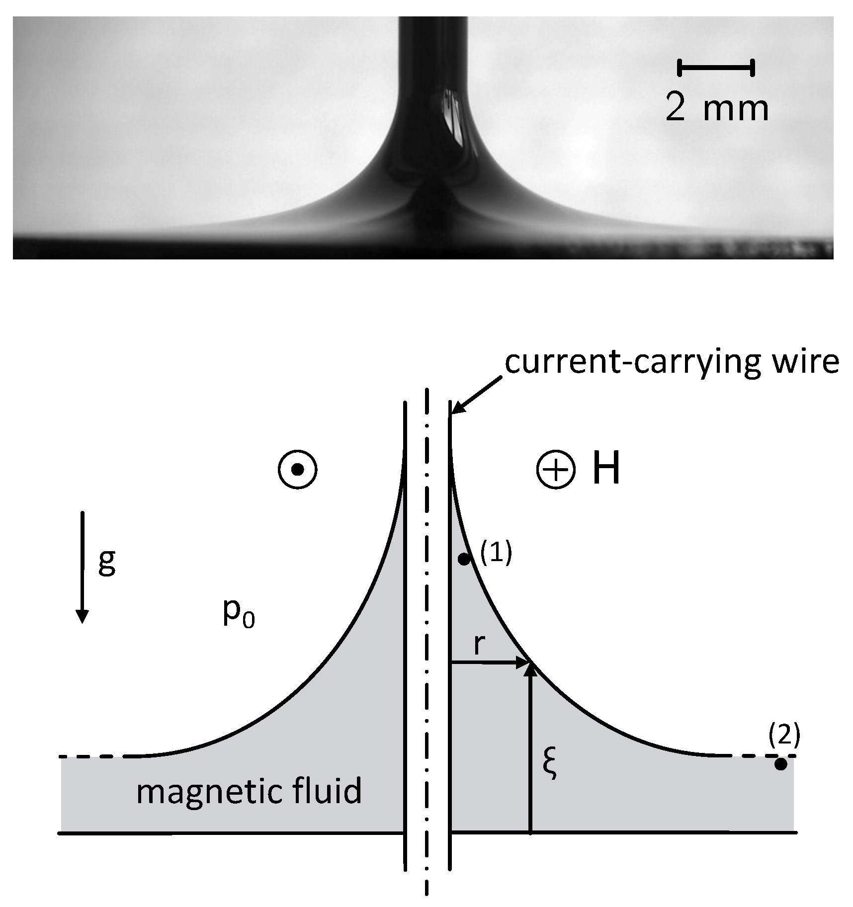
For the case of a vertical cylindrical current-carrying wire, considered here, the free surface forms a meniscus around the wire, as can be seen in the top part of
Figure 1. In equilibrium all contributions of pressure at point (1), close to the wire, are equal to all contributions at point (2), far away from it, see bottom part of
Figure 1. With the assumption that the free surface
and the magnetic field
of the wire tend to zero as
r goes to infinity, Equation (
4) reads
where the current through the wire is denoted by
I. The absolute value of the horizontal distance,
, the magnetic field as well as the magnetisation is given by
,
,
and
, respectively. Equation (
5) can be further reduced because the hydrostatic pressure is the same at both points and
due to
. The latter results from the fact that for
r to infinity the elevation of
diminishes. With a linear law of magnetisation,
, and the feature that only the azimuthal component of the magnetic field is nonzero, one finally yields an analytical equation for the free surface of the magnetic fluid [
16],
where
denotes the susceptibility of the MF and the primes the derivatives with respect to
r.
An analytical solution for the simple case of
was already given in [
15] (Chap. 5.4), but an analytical solution for the full problem (
6) is not yet available. The reason is the nonlinear character of the equation caused by the nonlinear structure of the curvature in the term of capillary pressure. Therefore, John et al. in [
16] proposed a transformation which regularises the problem and allows a numerical solution. Nevertheless, Equation (
6) is an approximation since the derivation of the Bernoulli equation assumes isothermal conditions as well as an irrotational and stationary flow field. Therefore, the aim of this study is to present numerical simulations of the underlying Navier–Stokes equation [
15] (Equation 5.2),
in three dimensions, where
denotes the dynamical viscosity of the magnetic fluid and
. No assumptions will be made about the flow field. The isothermal condition is kept for the simulations, but will be discussed separately in
Section 4.2. In the three-dimensional
r-
-
coordinate system, the Kelvin force density is given by
, where it was exploited that
and
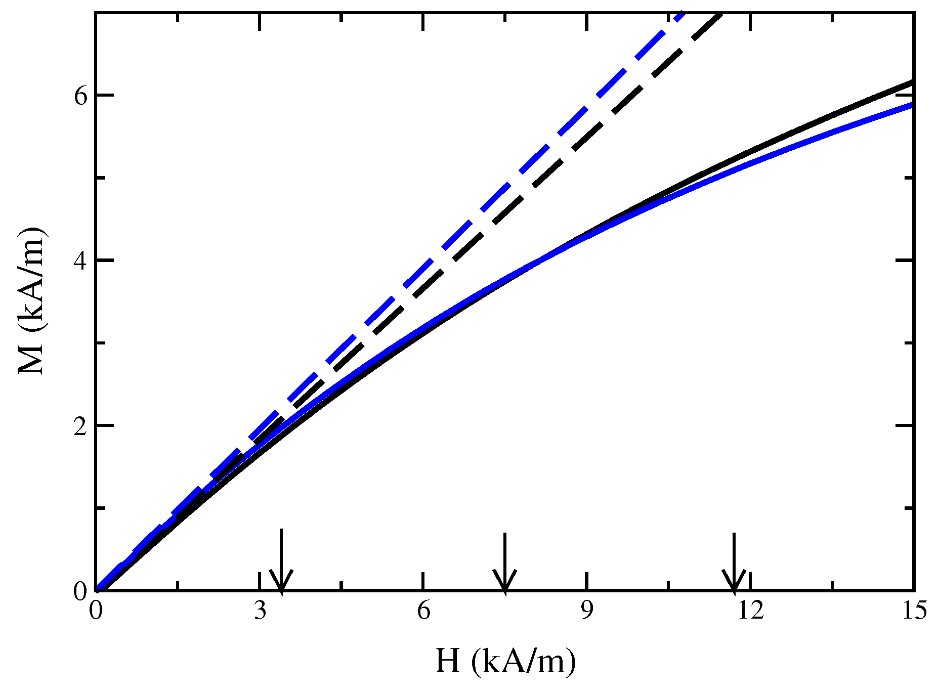
are co-linear. For the simulations, either a linear law of magnetisation is used or the experimental data of the nonlinear behaviour of the magnetisation (
Figure 2). The experiments were performed with the magnetic fluid EMG 909 (APG S21) having the material parameters
kg/m
(1140 kg/m
),
N/m (
N/m) and
(
[
17]. The dynamical viscosity is set to
kg/(m·s) since all tested values of
including the values given by the producer [
18] lead to identical menisci [
19]. The magnetic fluid EMG 909 (APG S21) is a light hydrocarbon oil-based (synthetic ester oil based) ferrofluid [
18] with a saturation magnetisation of
kA/m (
kA/m) and particles with a mean diameter of
nm (
nm) [
20]. The experimental set-up uses a wire with a radius of R = 0.95 mm and a welding transformer for the generation of the current which can achieve 100 Ampere in maximum [
17]. Three different strengths (small, moderate and large) of the current were applied: I = 20 A, I = 45 A and I = 70 A.
3. Numerical Methods
Extending the simulations in [
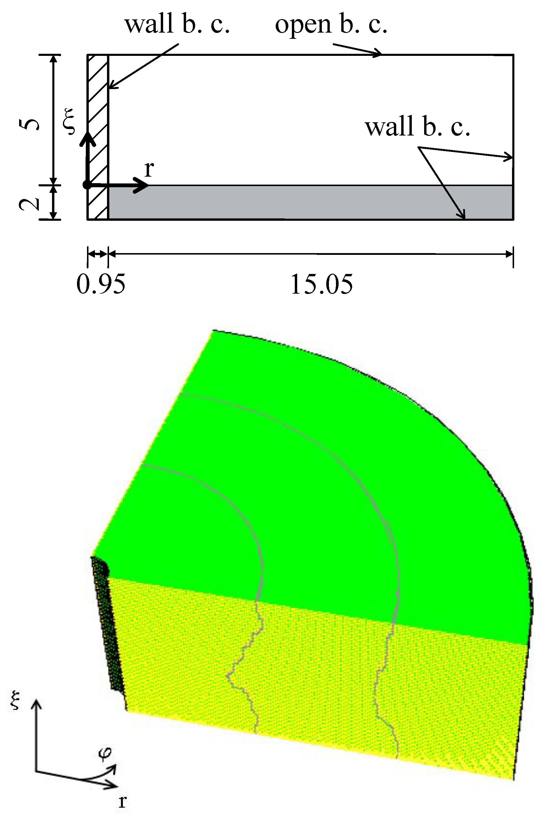
19], the numerics here is done in three dimensions. The numerical calculations were conducted with the commercial software package ANSYS FLUENT 13.0 using the finite volume method for the two phases fluid and air. The domain of calculation is a torus of rectangular cross-section with a width of 16 mm and a height of 7 mm according to the experimental set-up in [
17], where the origin is shifted by 2 mm in the vertical direction by the thickness of the layer of magnetic fluid, see
Figure 3 (top). No-slip boundary conditions (wall b. c.) are imposed at all boundaries, with the exception of the upper horizontal boundary, where a so called open boundary condition is present. This condition allows an unconstrained flow of air in or out of the system. By using a finite volume method the numerical results are affected by the so called “flotsam” generated during the reconstruction of the phase boundary between the MF and air. The flotsam is considerably reduced by the use of FLUENT’s GEO-Reconstruct method which is based on Youngs’ technique [
21]. That technique is superior to other approaches as a comparing study [
22] shows. Only in the column nearest to the wire a few cells of flotsam remain. As beyond a simulation time of
s in all tested cases this last flotsam does not move any more and does not influence the shape of the surface, it was removed. The change of the total mass of MF due to that removal can be neglected as the amount of flotsam is less than
% of the total mass of fluid.
FLUENT’s numerical method for modelling the surface tension is based on the continuum surface force (CSF) model proposed in [
23]. The CSF model uses the static angle of contact, established when the fluid is at rest. In agreement with this definition, the angle of contact of the MF with the wire was measured in [
17,
20]. By contrast, neither information about a change of this angle during the rise of the fluid at the wire nor any measurements of the angle of contact at the wall of the vessel are available [
17,
20]. Thus, the conducted numerics utilises static angles of contact only, where one of them is experimentally known.
To reduce the computing time only a quarter of the torus, supplemented with suitable conditions on the symmetry, was actually calculated. The area of calculation is divided in vertical direction into 50 cells, in radial direction into 480 cells and in azimutal direction at the outer rim into 250 cells. That sums totally up to approximately
cells. That quarter was divided into three parts automatically by FLUENT, see
Figure 3 (bottom), to allow a parallel calculation in each of them. The final computing time of a quarter of the torus summed up to two and a half days which corresponds to a real time of
s.
The system calculated numerically here constitutes a model system with respect to geometry and the analytically known magnetic field. With such a model system, the quality of the numerics can be tested, particularly if experimental results are available. In that way, one receives knowledge about the strengths and weaknesses of the numerics of free surfaces of magnetic fluids which is helpful for the numerics of non-model systems as in the case of magnetic field concentrators [
24] or locomotion systems [
25].
5. Discussion
In this section, the consequences of the absence of isothermal conditions are discussed in detail. An increase of the temperature, particularly close to the wire, will generate a raised evaporation. The resulting increase of the volume concentration of magnetic particles and the increase of the temperature itself cause different consequences for magnetisation and surface tension.
The strength of the magnetisation depends on two contrary dependencies: the increased volume concentration would increase the magnetisation, whereas the increase of the temperature would decrease the magnetisation; which dependency wins over the other is not clear, as measurements of the magnetisation as a function of the temperature, as in [
27], did not determine in parallel the volume concentration. A similar behaviour applies to the density: an increase of the density by an increase in the volume concentration stays contrary to a decrease due to a higher temperature.
Furthermore, the surface tension is a critical factor in several respects, where two of them are related to changes of the temperature. First, an evaporation of the carrier liquid leads to a higher volume concentration of the magnetic particles which causes an increase of the surface tension as measured in [
28]. Second, and simultaneously, a higher temperature brings forth a reduction of the surface tension. As no particular measurements of the temperature dependence of the surface tension of magnetic fluids are known, to the best knowledge of the authors, we are referring to recent measurements for binary mixtures [
29], which confirm this dependence. With respect to magnetic fluids, it is an open question which of the two effects dominates the other one. Third, there is the size of the angle of contact at the wire. That angle is related to the surface tension between magnetic fluid and air by Young’s equation [
30] expressing a necessary boundary condition for the fluid. Therefore a measurement of this angle during the experiments constitutes a vital information and would be an additional input for future numerical simulations, supported by the findings in [
17] about the ferrofluid–air interface.
6. Summary and Future Work
Three-dimensional calculations of the meniscus of a magnetic fluid around a current carrying vertical and cylindrical wire are presented. Based on the material properties of experimentally used magnetic fluids, the numerically determined menisci are compared with the experimentally measured one. The comparison is made for a linear law of magnetisation as well as for the experimentally measured nonlinear magnetisation curve.
For a linear law of magnetisation, and for low as well as for moderate strengths of the current, the profiles agree satisfyingly up to 2 mm to the wire. Closer to the wire, and for high values of the current, the agreement is not so satisfying. Therefore, a nonlinear law of magnetisation was tested. The overall picture is that the maximal deviation for the nonlinear law of magnetisation is somehow larger than for the linear law. That is at first view counterintuitive since the nonlinear law of magnetisation is closer to the real properties of a magnetic fluid than a linear law. To resolve that puzzle, the thermal conditions in the experiment and in the simulations, respectively, come into play. For isothermal conditions, as present in the simulations, the linear law of magnetisation yields larger magnetisations than the nonlinear law with the exception of rather small magnetic fields. In the real experiment, the temperature is higher close to the wire than further away. An increase in the temperature causes two contrary dependencies: on the one hand, an increase of the magnetisation by an increased volume concentration of magnetic particles caused by evaporation, and on the other hand, a decrease of the magnetisation by the increased temperature itself. If the first dependency wins for the used magnetic fluids, the real magnetisation close to the wire is higher than the magnetisation further away, and higher magnetisations close to the wire generate a better agreement as the simulations with the less realistic linear law of magnetisation show. The fact that evaporation has a relevant influence on the results shows the better agreement for the fluid APG S21 with a lower evaporation rate in comparison with the fluid EMG 909.
The thermal aspects of the system turn out to be the most relevant ones in order to bridge the remaining gap between the real experiment and the model used for the calculations. A rising of the temperature modifies magnetisation as well as surface tension. In which way the modification takes place is not yet finally clarified. On the one hand, the increased temperature leads to a decrease of magnetisation and surface tension, whereas the increased volume concentration of magnetic particles, due to the raised evaporation, leads to an increase of both quantities. This situation directs the future work in several aspects.
From a numerical point of view, it would be desirable to implement a coupled thermal model since the present numerical model is limited to an isothermal situation. An essential requirement are reliable measurements of the dependence of the surface tension on temperature, as such measurements are not available presently. A parallel determination of the volume concentration of magnetic particles would deepen the understanding of the temperature effects. The same kind of measurements should be applied on the magnetisation. In this way, the magnetic liquids are suitable characterised if used for this type of experiments.
From an experimental point of view, a control of the temperature is considered essential. The aim should be to keep the temperature as best as possible constant, particularly in the vicinity of the wire. Therefore, a cooling of the wire as well as a tempering of the entire set-up would be advantageous in order to keep the differences in temperature as small as possible. To quantity the temperature control, measurements of the temperature of the wire and the fluid, the latter at different distances to the wire and different circumferential positions, should be implemented. Also, a measurement of the angle of contact of the magnetic fluid at the wire would add vital information about the behaviour of the surface at and close to the wire.
That all should lead to a better characterisation of the system and an improved agreement between experiment and numerics.


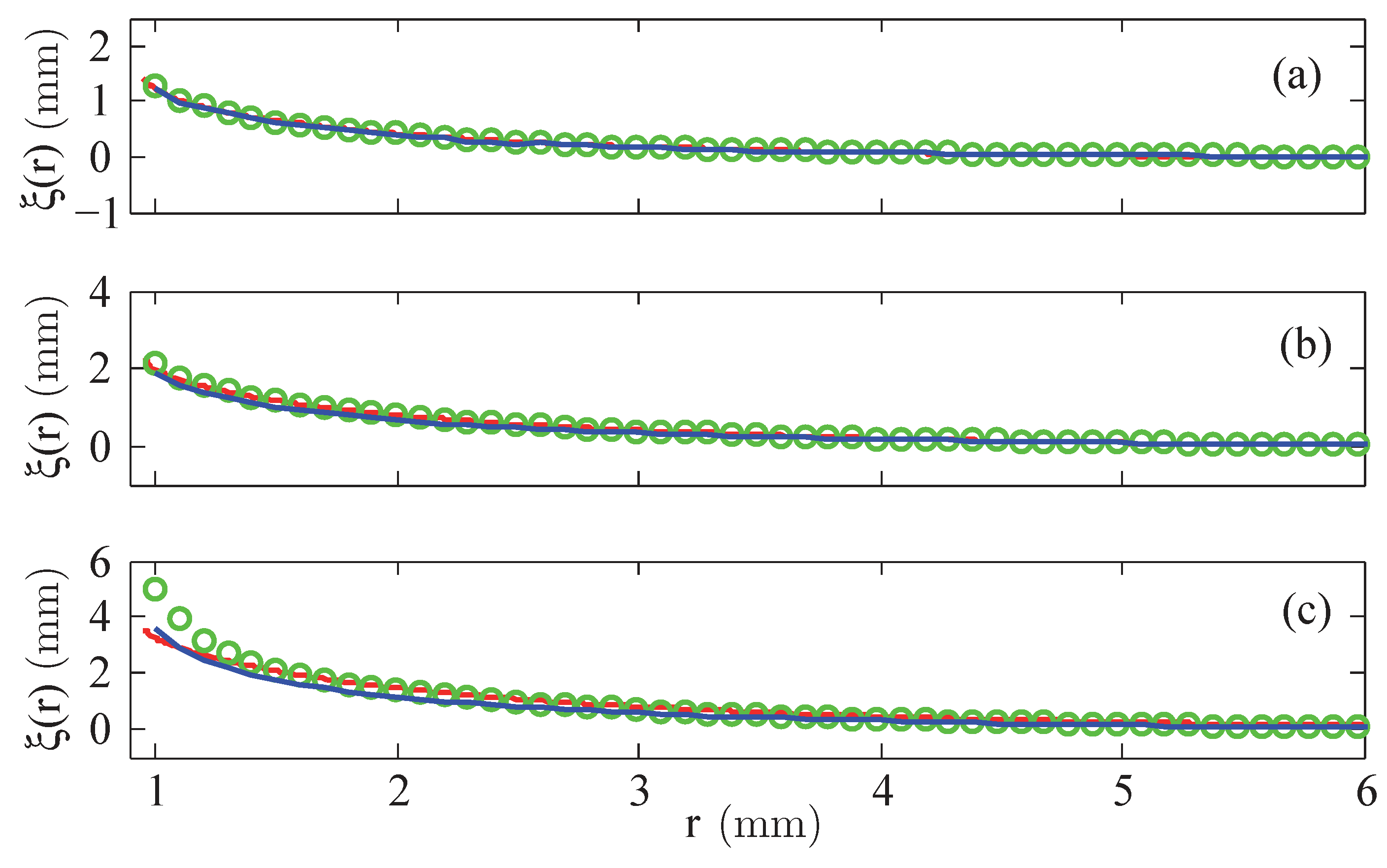
 ) and (
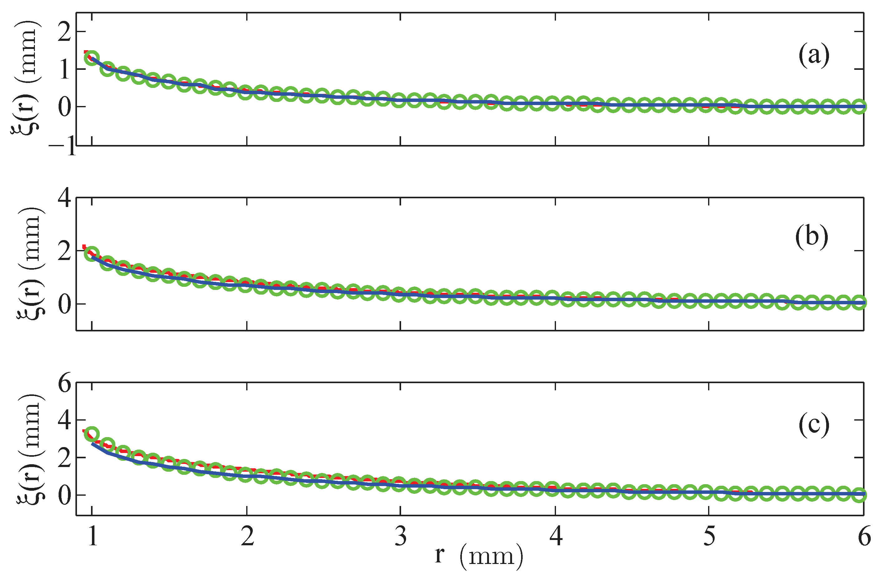
  ) versus the experimentally determined surfaces (
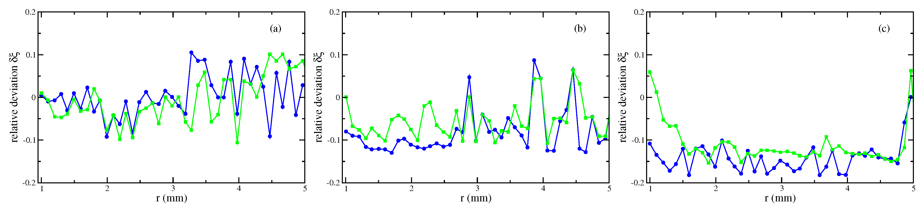
  ). (a) kA/m, (b) kA/m, and (c) kA/m at mm.

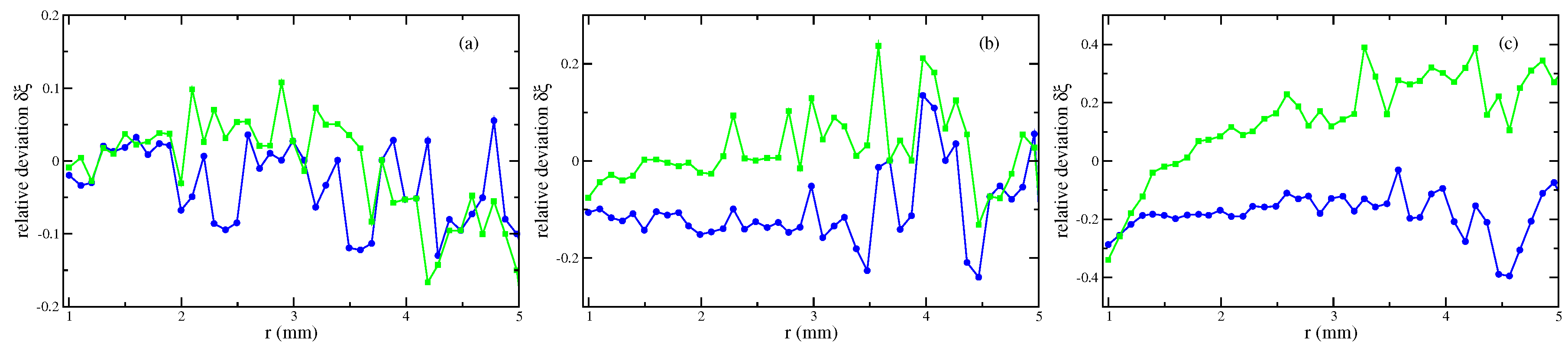
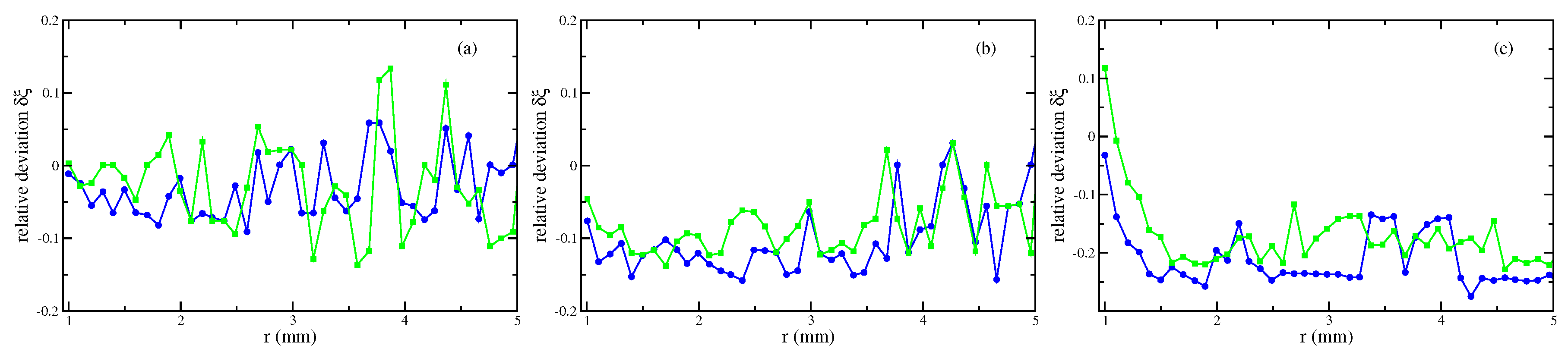
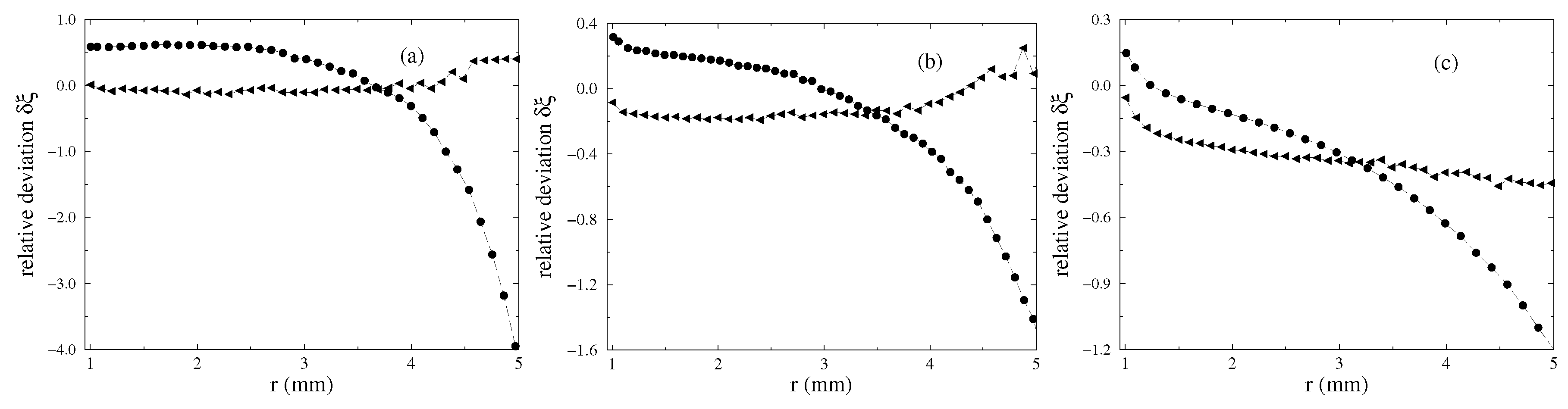
 ). (a) kA/m, (b) kA/m and (c) kA/m at mm. The lines are guides for the eye. Note the different scales at the axes of ordinates.