Robust Multiscale Identification of Apparent Elastic Properties at Mesoscale for Random Heterogeneous Materials with Multiscale Field Measurements


Abstract
1. Introduction
1.1. Overview of Inverse Methods for the Mechanical Characterization of Micro/Meso-Structural Properties
1.2. Multiscale Statistical Identification Method
1.3. Drawbacks and Limitations of the Multiscale Identification Method
1.4. Improvements of the Multiscale Identification Method and Novelty of the Paper
1.5. Outline of the Paper
2. Assumptions for Solving the Multiscale Statistical Inverse Problem
- there exists a scale separation between macroscale and mesoscale, so that a mesoscopic subdomain can be defined and for which the dimensions are sufficiently large with respect to the size of the heterogeneities and sufficiently small with respect to the size of the macroscopic domain. Such a mesoscopic subdomain can then be considered as a representative volume element;
- the random apparent elasticity tensor field at mesoscale is the restriction to one or more bounded mesoscopic subdomain(s) of a second-order stationary random field indexed by , and consequently the mean function of the random elasticity field at mesoscale is independent of the spatial coordinates;
- the random apparent elasticity tensor field at mesoscale is ergodic in average in the mean-square sense, so that the homogenized elasticity tensor at macroscale calculated by stochastic homogenization of the random apparent elasticity field in a mesoscopic subdomain corresponding to a representative volume element can be considered as almost deterministic, in the sense that (i) its spatial average reaches an asymptotic convergence with a very high level of probability for a sufficiently large mesoscopic subdomain size, and therefore (ii) its level of statistical fluctuations around its mean function at macroscale can be considered as negligible, thus yielding a deterministic homogenized elasticity tensor at macroscale.
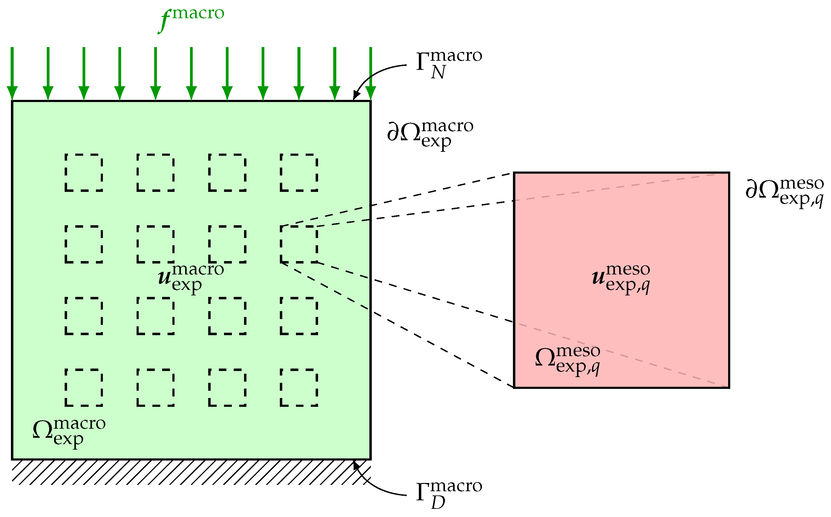
3. Multiscale Experimental Test Configuration
4. Prior Multiscale Stochastic Model and Its Hyperparameters
5. Objectives and Strategy for Solving the Multiscale Statistical Inverse Problem
5.1. Objectives of the Multiscale Statistical Inverse Problem
5.2. Strategy for Solving the Multiscale Statistical Inverse Problem
- A macroscopic numerical indicator , dedicated to the identification of parameter , that allows for quantifying the distance between the experimental strain field associated to the experimental displacement field measured at macroscale in the macroscopic domain and the strain field associated to the displacement field computed from a deterministic homogeneous linear elasticity boundary value problem (with both Dirichlet and Neumann boundary conditions) that models the experimental test configuration at macroscale and involves the unknown deterministic elasticity tensor ;
- A mesoscopic numerical indicator , dedicated to the identification of hyperparameter , that allows for quantifying the distance between a pseudo-dispersion coefficient modeling the level of spatial fluctuations of the experimental strain field associated to the experimental displacement field measured at mesoscale in a mesoscopic domain of observation , and a random pseudo-dispersion coefficient representing the level of statistical fluctuations of the random strain field associated to the random displacement field computed from a stochastic heterogeneous linear elasticity boundary value problem (with only Dirichlet boundary conditions) that models the experimental test configuration at mesoscale and involves the random elasticity tensor field with an unknown level of statistical fluctuations that must be identified;
- Another mesoscopic numerical indicator , dedicated to the identification of hyperparameter , that allows for quantifying the distance between the 3 different pseudo-spatial correlation lengths of the experimental strain field in each spatial direction, measured at mesoscale in a mesoscopic domain of observation , and the 3 pseudo-spatial correlation lengths of the random strain field in each spatial direction, computed from the same mesoscopic stochastic boundary value problem as for for which the random elasticity tensor field has a spatial correlation structure induced and characterized by an unknown vector of spatial correlation lengths that must be identified;
- A multiscale numerical indicator , dedicated to the identification of hyperparameter , that allows for quantifying the distance between the homogeneous deterministic elasticity tensor at macroscale and the effective elasticity tensor resulting from a computational stochastic homogenization in a representative volume element at mesoscale of the random elasticity tensor field whose mean function is unknown and must be identify.
6. Construction of the Numerical Indicators for Solving the Multiscale Statistical Inverse Problem
6.1. Deterministic Macroscopic Boundary Value Problem for the Macroscopic Indicator
6.2. Stochastic Mesoscopic Boundary Value Problem for the Mesoscopic Indicators
6.3. Macroscopic Numerical Indicator
6.4. Mesoscopic and Multiscale Numerical Indicators
6.4.1. Mesoscopic Numerical Indicator Associated to the Dispersion Parameter
6.4.2. Mesoscopic Numerical Indicator Associated to the Spatial Correlation Lengths
6.4.3. Multiscale Numerical Indicator Associated to Computational Stochastic Homogenization
6.5. Comments
7. Multiscale Statistical Inverse Problem Formulated as a Multi-Objective Optimization Problem
- a macroscale inverse problem formulated as a single-objective optimization problem that consists in calculating the optimal value of parameter in that minimizes the macroscopic numerical indicator , that is
- a mesoscale statistical inverse problem formulated as a multi-objective optimization problem that consists in calculating the optimal value of hyperparameter in that minimizes the two mesoscopic numerical indicators and as well as the multiscale numerical indicator simultaneously, that iswhere is the (vector-valued) multi-objective cost function defined for any vector by
8. Numerical Methods for Solving the Multi-Objective Optimization Problem
9. Probabilistic Model for a Robust Identification of the Hyperparameters
10. Numerical Validation of the Multiscale Identification Method on In Silico Materials in 2D Plane Stress and 3D Linear Elasticity
10.1. Validation on an In Silico Specimen in Compression Test in 2D Plane Stress Linear Elasticity
10.1.1. Parameterization of the Macroscopic and Mesoscopic Models
10.1.2. Resolution of the Single-Objective Optimization Problem at Macroscale
10.1.3. Resolution of the Multi-Objective Optimization Problem at Mesoscale
10.2. Validation on an In Silico Specimen in Compression Test in 3D Linear Elasticity
10.2.1. Parameterization of the Macroscopic and Mesoscopic Models
10.2.2. Resolution of the Single-Objective Optimization Problem at Macroscale
10.2.3. Resolution of the Multi-Objective Optimization Problem at Mesoscale
11. Numerical Application of the Multiscale Identification Method to Real Beef Cortical Bone in Plane Stress Linear Elasticity
11.1. Parameterization of the Macroscopic and Mesoscopic Models
11.2. Numerical Results of the Multiscale Statistical Inverse Identification
11.2.1. Resolution of the Single-Objective Optimization Problem at Macroscale
11.2.2. Resolution of the Multi-Objective Optimization Problem at Mesoscale
12. Conclusions
Author Contributions
Funding
Acknowledgments
Conflicts of Interest
Abbreviations
| a.s. | almost surely |
| RVE | Representative Volume Element |
| CCD | Charge-Coupled Device |
| CMOS | Complementary Metal-Oxide-Semiconductor |
| DIC | Digital Image Correlation |
| DVC | Digital Volume Correlation |
| CT | micro-Computed Tomography |
| MRI | Magnetic Resonance Imaging |
| OCT | Optical Coherence Tomography |
| LS | Least Squares |
| MLE | Maximum Likelihood Estimation |
| MaxEnt | Maximum Entropy |
| KL | Karhunen-Loève |
| PC | Polynomial Chaos |
| FP | Fixed-Point |
| GA | Genetic Algorithm |
| FEM | Finite Element Method |
References
- Torquato, S. Random Heterogeneous Materials: Microstructure and Macroscopic Properties; Springer: New York, NY, USA, 2002; Volume 16. [Google Scholar] [CrossRef]
- Jeulin, D. Microstructure modeling by random textures. J. Microsc. Spectrosc. Electron. 1987, 12, 133–140. [Google Scholar]
- Jeulin, D. Morphological modeling of images by sequential random functions. Signal Process. 1989, 16, 403–431. [Google Scholar] [CrossRef]
- Jeulin, D. Random texture models for material structures. Stat. Comput. 2000, 10, 121–132. [Google Scholar] [CrossRef]
- Jeulin, D. Random Structure Models for Homogenization and Fracture Statistics. In Mechanics of Random and Multiscale Microstructures; Jeulin, D., Ostoja-Starzewski, M., Eds.; Springer: Vienna, Austria, 2001; pp. 33–91. [Google Scholar] [CrossRef]
- Jeulin, D. Morphology and effective properties of multi-scale random sets: A review. C. R. Méc. 2012, 340, 219–229. [Google Scholar] [CrossRef]
- Pan, B.; Qian, K.; Xie, H.; Asundi, A. Two-dimensional digital image correlation for in-plane displacement and strain measurement: A review. Meas. Sci. Technol. 2009, 20, 062001. [Google Scholar] [CrossRef]
- Sutton, M.A.; Orteu, J.J.; Schreier, H. Image Correlation for Shape, Motion and Deformation Measurements: Basic Concepts, Theory and Applications; Springer: Boston, MA, USA, 2009. [Google Scholar] [CrossRef]
- Hild, F.; Roux, S. Optical Methods for Solid Mechanics. A Full-Field Approach; Chapter Digital Image Correlation; Wiley-VCH: Weinheim, Germany, 2012; pp. 183–228. [Google Scholar]
- Kahn-Jetter, Z.L.; Jha, N.K.; Bhatia, H. Optimal image correlation in experimental mechanics. Opt. Eng. 1994, 33, 1099–1105. [Google Scholar] [CrossRef]
- Vendroux, G.; Knauss, W.G. Submicron deformation field measurements: Part 1. Developing a digital scanning tunneling microscope. Exp. Mech. 1998, 38, 18–23. [Google Scholar] [CrossRef]
- Vendroux, G.; Knauss, W.G. Submicron deformation field measurements: Part 2. Improved digital image correlation. Exp. Mech. 1998, 38, 86–92. [Google Scholar] [CrossRef]
- Hild, F.; Roux, S. Digital Image Correlation: From Displacement Measurement to Identification of Elastic Properties—A Review. Strain 2006, 42, 69–80. [Google Scholar] [CrossRef]
- Roux, S.; Hild, F. Digital Image Mechanical Identification (DIMI). Exp. Mech. 2008, 48, 495–508. [Google Scholar] [CrossRef]
- Réthoré, J.; Tinnes, J.P.; Roux, S.; Buffière, J.Y.; Hild, F. Extended three-dimensional digital image correlation (X3D-DIC). C. R. Méc. 2008, 336, 643–649. [Google Scholar] [CrossRef]
- Bornert, M.; Valès, F.; Gharbi, H.; Nguyen Minh, D. Multiscale Full-Field Strain Measurements for Micromechanical Investigations of the Hydromechanical Behaviour of Clayey Rocks. Strain 2010, 46, 33–46. [Google Scholar] [CrossRef]
- Constantinescu, A. On the identification of elastic moduli from displacement-force boundary measurements. Inverse Probl. Eng. 1995, 1, 293–313. [Google Scholar] [CrossRef]
- Baxter, S.C.; Graham, L.L. Characterization of Random Composites Using Moving-Window Technique. J. Eng. Mech. 2000, 126, 389–397. [Google Scholar] [CrossRef]
- Geymonat, G.; Hild, F.; Pagano, S. Identification of elastic parameters by displacement field measurement. C. R. Méc. 2002, 330, 403–408. [Google Scholar] [CrossRef]
- Geymonat, G.; Pagano, S. Identification of Mechanical Properties by Displacement Field Measurement: A Variational Approach. Meccanica 2003, 38, 535–545. [Google Scholar] [CrossRef]
- Graham, L.; Gurley, K.; Masters, F. Non-Gaussian simulation of local material properties based on a moving-window technique. Probab. Eng. Mech. 2003, 18, 223–234. [Google Scholar] [CrossRef]
- Bonnet, M.; Constantinescu, A. Inverse problems in elasticity. Inverse Probl. 2005, 21, R1–R50. [Google Scholar] [CrossRef]
- Avril, S.; Pierron, F. General framework for the identification of constitutive parameters from full-field measurements in linear elasticity. Int. J. Solids Struct. 2007, 44, 4978–5002. [Google Scholar] [CrossRef]
- Avril, S.; Bonnet, M.; Bretelle, A.S.; Grédiac, M.; Hild, F.; Ienny, P.; Latourte, F.; Lemosse, D.; Pagano, S.; Pagnacco, E.; et al. Overview of Identification Methods of Mechanical Parameters Based on Full-field Measurements. Exp. Mech. 2008, 48, 381. [Google Scholar] [CrossRef]
- Flannery, B.P.; Deckman, H.W.; Roberge, W.G.; D’amico, K.L. Three-Dimensional X-ray Microtomography. Science 1987, 237, 1439–1444. [Google Scholar] [CrossRef] [PubMed]
- Kak, A.C.; Slaney, M. Principles of Computerized Tomographic Imaging; IEEE Press: Piscataway, NJ, USA, 1988. [Google Scholar]
- Baruchel, J.; Buffiere, J.Y.; Maire, E. X-ray Tomography in Material Science; Hermes Science Publications: Paris, France, 2000. [Google Scholar]
- Stock, S.R. Recent advances in X-ray microtomography applied to materials. Int. Mater. Rev. 2008, 53, 129–181. [Google Scholar] [CrossRef]
- Desrues, J.; Viggiani, G.; Besuelle, P. Advances in X-ray Tomography for Geomaterials; John Wiley & Sons: Hoboken, NJ, USA, 2010; Volume 118. [Google Scholar] [CrossRef]
- Maire, E.; Withers, P.J. Quantitative X-ray tomography. Int. Mater. Rev. 2014, 59, 1–43. [Google Scholar] [CrossRef]
- van den Elsen, P.A.; Pol, E.D.; Viergever, M.A. Medical image matching—A review with classification. IEEE Eng. Med. Biol. Mag. 1993, 12, 26–39. [Google Scholar] [CrossRef]
- Maintz, J.; Viergever, M.A. A survey of medical image registration. Med. Image Anal. 1998, 2, 1–36. [Google Scholar] [CrossRef]
- Liang, Z.P.; Lauterbur, P.C. Principles of Magnetic Resonance Imaging: A Signal Processing Perspective; IEEE Press Series in Biomedical Engineering; SPIE Optical Engineering Press: Bellingham, WA, USA, 2000. [Google Scholar]
- Hill, D.L.G.; Batchelor, P.G.; Holden, M.; Hawkes, D.J. Medical image registration. Phys. Med. Biol. 2001, 46, R1–R45. [Google Scholar] [CrossRef]
- Beaurepaire, E.; Boccara, A.C.; Lebec, M.; Blanchot, L.; Saint-Jalmes, H. Full-field optical coherence microscopy. Opt. Lett. 1998, 23, 244–246. [Google Scholar] [CrossRef]
- Schmitt, J.M. Optical coherence tomography (OCT): A review. IEEE J. Sel. Top. Quantum Electron. 1999, 5, 1205–1215. [Google Scholar] [CrossRef]
- Fercher, A.F. Optical coherence tomography–development, principles, applications. Z. Med. Phys. 2010, 20, 251–276. [Google Scholar] [CrossRef]
- Gambichler, T.; Jaedicke, V.; Terras, S. Optical coherence tomography in dermatology: Technical and clinical aspects. Arch. Dermatol. Res. 2011, 303, 457–473. [Google Scholar] [CrossRef]
- Popescu, D.P.; Choo-Smith, L.P.; Flueraru, C.; Mao, Y.; Chang, S.; Disano, J.; Sherif, S.; Sowa, M.G. Optical coherence tomography: Fundamental principles, instrumental designs and biomedical applications. Biophys. Rev. 2011, 3, 155. [Google Scholar] [CrossRef]
- Bay, B.K.; Smith, T.S.; Fyhrie, D.P.; Saad, M. Digital volume correlation: Three-dimensional strain mapping using X-ray tomography. Exp. Mech. 1999, 39, 217–226. [Google Scholar] [CrossRef]
- Verhulp, E.; Rietbergen, B.; Huiskes, R. A three-dimensional digital image correlation technique for strain measurements in microstructures. J. Biomech. 2004, 37, 1313–1320. [Google Scholar] [CrossRef] [PubMed]
- Bay, B.K. Methods and applications of digital volume correlation. J. Strain Anal. Eng. Des. 2008, 43, 745–760. [Google Scholar] [CrossRef]
- Roux, S.; Hild, F.; Viot, P.; Bernard, D. Three-dimensional image correlation from X-ray computed tomography of solid foam. Compos. Part A Appl. Sci. Manuf. 2008, 39, 1253–1265. [Google Scholar] [CrossRef]
- Rannou, J.; Limodin, N.; Réthoré, J.; Gravouil, A.; Ludwig, W.; Baïetto-Dubourg, M.C.; Buffière, J.Y.; Combescure, A.; Hild, F.; Roux, S. Three dimensional experimental and numerical multiscale analysis of a fatigue crack. Comput. Methods Appl. Mech. Eng. 2010, 199, 1307–1325. [Google Scholar] [CrossRef]
- Madi, K.; Tozzi, G.; Zhang, Q.; Tong, J.; Cossey, A.; Au, A.; Hollis, D.; Hild, F. Computation of full-field displacements in a scaffold implant using digital volume correlation and finite element analysis. Med. Eng. Phys. 2013, 35, 1298–1312. [Google Scholar] [CrossRef] [PubMed]
- Roberts, B.C.; Perilli, E.; Reynolds, K.J. Application of the digital volume correlation technique for the measurement of displacement and strain fields in bone: A literature review. J. Biomech. 2014, 47, 923–934. [Google Scholar] [CrossRef]
- Fedele, R.; Ciani, A.; Fiori, F. X-ray Microtomography under Loading and 3D-Volume Digital Image Correlation: A Review. Fundam. Inform. 2014, 135, 171–197. [Google Scholar] [CrossRef]
- Hild, F.; Bouterf, A.; Chamoin, L.; Leclerc, H.; Mathieu, F.; Neggers, J.; Pled, F.; Tomičević, Z.; Roux, S. Toward 4D Mechanical Correlation. Adv. Model. Simul. Eng. Sci. 2016, 3, 17. [Google Scholar] [CrossRef]
- Bouterf, A.; Adrien, J.; Maire, E.; Brajer, X.; Hild, F.; Roux, S. Identification of the crushing behavior of brittle foam: From indentation to oedometric tests. J. Mech. Phys. Solids 2017, 98, 181–200. [Google Scholar] [CrossRef]
- Buljac, A.; Jailin, C.; Mendoza, A.; Neggers, J.; Taillandier-Thomas, T.; Bouterf, A.; Smaniotto, B.; Hild, F.; Roux, S. Digital Volume Correlation: Review of Progress and Challenges. Exp. Mech. 2018, 58, 661–708. [Google Scholar] [CrossRef]
- Desceliers, C.; Ghanem, R.; Soize, C. Maximum likelihood estimation of stochastic chaos representations from experimental data. Int. J. Numer. Methods Eng. 2006, 66, 978–1001. [Google Scholar] [CrossRef]
- Ghanem, R.G.; Doostan, A. On the construction and analysis of stochastic models: Characterization and propagation of the errors associated with limited data. J. Comput. Phys. 2006, 217, 63–81. [Google Scholar] [CrossRef]
- Desceliers, C.; Soize, C.; Ghanem, R. Identification of Chaos Representations of Elastic Properties of Random Media Using Experimental Vibration Tests. Comput. Mech. 2007, 39, 831–838. [Google Scholar] [CrossRef]
- Marzouk, Y.M.; Najm, H.N.; Rahn, L.A. Stochastic spectral methods for efficient Bayesian solution of inverse problems. J. Comput. Phys. 2007, 224, 560–586. [Google Scholar] [CrossRef]
- Arnst, M.; Clouteau, D.; Bonnet, M. Inversion of probabilistic structural models using measured transfer functions. Comput. Methods Appl. Mech. Eng. 2008, 197, 589–608. [Google Scholar] [CrossRef]
- Das, S.; Ghanem, R.; Spall, J.C. Asymptotic Sampling Distribution for Polynomial Chaos Representation of Data: A Maximum Entropy and Fisher information approach. In Proceedings of the 45th IEEE Conference on Decision and Control, San Diego, CA, USA, 13–15 December 2006; pp. 4139–4144. [Google Scholar] [CrossRef]
- Das, S.; Ghanem, R.; Finette, S. Polynomial chaos representation of spatio-temporal random fields from experimental measurements. J. Comput. Phys. 2009, 228, 8726–8751. [Google Scholar] [CrossRef]
- Desceliers, C.; Soize, C.; Grimal, Q.; Talmant, M.; Naili, S. Determination of the random anisotropic elasticity layer using transient wave propagation in a fluid-solid multilayer: Model and experiments. J. Acoust. Soc. Am. 2009, 125, 2027–2034. [Google Scholar] [CrossRef]
- Guilleminot, J.; Soize, C.; Kondo, D. Mesoscale probabilistic models for the elasticity tensor of fiber reinforced composites: Experimental identification and numerical aspects. Mech. Mater. 2009, 41, 1309–1322. [Google Scholar] [CrossRef]
- Ma, X.; Zabaras, N. An efficient Bayesian inference approach to inverse problems based on an adaptive sparse grid collocation method. Inverse Probl. 2009, 25, 035013. [Google Scholar] [CrossRef]
- Marzouk, Y.M.; Najm, H.N. Dimensionality reduction and polynomial chaos acceleration of Bayesian inference in inverse problems. J. Comput. Phys. 2009, 228, 1862–1902. [Google Scholar] [CrossRef]
- Arnst, M.; Ghanem, R.; Soize, C. Identification of Bayesian posteriors for coefficients of chaos expansions. J. Comput. Phys. 2010, 229, 3134–3154. [Google Scholar] [CrossRef][Green Version]
- Das, S.; Spall, J.C.; Ghanem, R. Efficient Monte Carlo computation of Fisher information matrix using prior information. Comput. Stat. Data Anal. 2010, 54, 272–289. [Google Scholar] [CrossRef]
- Ta, Q.A.; Clouteau, D.; Cottereau, R. Modeling of random anisotropic elastic media and impact on wave propagation. Eur. J. Comput. Mech. 2010, 19, 241–253. [Google Scholar] [CrossRef]
- Soize, C. Identification of high-dimension polynomial chaos expansions with random coefficients for non-Gaussian tensor-valued random fields using partial and limited experimental data. Comput. Methods Appl. Mech. Eng. 2010, 199, 2150–2164. [Google Scholar] [CrossRef]
- Soize, C. A computational inverse method for identification of non-Gaussian random fields using the Bayesian approach in very high dimension. Comput. Methods Appl. Mech. Eng. 2011, 200, 3083–3099. [Google Scholar] [CrossRef]
- Lawson, C.; Hanson, R. Solving Least Squares Problems; Society for Industrial and Applied Mathematics: Philadelphia, PA, USA, 1995. [Google Scholar] [CrossRef]
- Soize, C. Uncertainty Quantification: An Accelerated Course with Advanced Applications in Computational Engineering, 1st ed.; Interdisciplinary Applied Mathematics; Springer: Berlin, Germany, 2017; Volume 47. [Google Scholar] [CrossRef]
- Serfling, R. Approximation Theorems of Mathematical Statistics; Wiley: New York, NY, USA, 1980. [Google Scholar] [CrossRef]
- Papoulis, A.; Pillai, S.U. Probability, Random Variables, and Stochastic Processes, 4th ed.; McGraw-Hill Higher Education: New York, NY, USA, 2002. [Google Scholar]
- Spall, J.C. Introduction to Stochastic Search and Optimization: Estimation, Simulation, and Control; John Wiley & Sons: Hoboken, NJ, USA, 2005; Volume 65. [Google Scholar] [CrossRef]
- Jaynes, E.T. Information Theory and Statistical Mechanics. Phys. Rev. 1957, 106, 620–630. [Google Scholar] [CrossRef]
- Jaynes, E.T. Information Theory and Statistical Mechanics. II. Phys. Rev. 1957, 108, 171–190. [Google Scholar] [CrossRef]
- Sobezyk, K.; Trȩbicki, J. Maximum entropy principle in stochastic dynamics. Probab. Eng. Mech. 1990, 5, 102–110. [Google Scholar] [CrossRef]
- Kapur, J.N.; Kesavan, H.K. Entropy Optimization Principles and Their Applications. In Entropy and Energy Dissipation in Water Resources; Singh, V.P., Fiorentino, M., Eds.; Springer: Dordrecht, The Netherlands, 1992; pp. 3–20. [Google Scholar] [CrossRef]
- Jumarie, G. Maximum Entropy, Information Without Probability and Complex Fractals: Classical and Quantum Approach; Fundamental Theories of Physics; Springer: Dordrecht, The Netherlands, 2000; Volume 112. [Google Scholar] [CrossRef]
- Jaynes, E.T. Probability Theory: The Logic of Science; Cambridge University Press: Cambridge, UK, 2003. [Google Scholar]
- Cover, T.M.; Thomas, J.A. Elements of Information Theory; A Wiley-Interscience Publication; Wiley: New York, NY, USA, 2006. [Google Scholar]
- Bowman, A.W.; Azzalini, A. Applied Smoothing Techniques for Data Analysis; Oxford University Press: Oxford, UK, 1997. [Google Scholar]
- Beck, J.L.; Katafygiotis, L.S. Updating Models and Their Uncertainties. I: Bayesian Statistical Framework. J. Eng. Mech. 1998, 124, 455–461. [Google Scholar] [CrossRef]
- Bernardo, J.M.; Smith, A.F.M. Bayesian Theory. Meas. Sci. Technol. 2001, 12, 221. [Google Scholar] [CrossRef]
- Congdon, P. Bayesian Statistical Modelling, 2nd ed.; Wiley Series in Probability and Statistics; John Wiley and Sons, Ltd.: Chichester, UK, 2007. [Google Scholar]
- Carlin, B.P.; Louis, T.A. Bayesian Methods for Data Analysis, 3rd ed.; Texts in Statistical Science; CRC Press: Boca Raton, FL, USA, 2009. [Google Scholar]
- Stuart, A.M. Inverse problems: A Bayesian perspective. Acta Numer. 2010, 19, 451–559. [Google Scholar] [CrossRef]
- Tan, M.T.; Tian, G.L.; Ng, K.W. Bayesian Missing Data Problems: EM, Data Augmentation and Noniterative Computation; Formerly CIP; Chapman & Hall/CRC Press: Boca Raton, FL, USA, 2010. [Google Scholar]
- Rappel, H.; Beex, L.A.A.; Hale, J.S.; Noels, L.; Bordas, S.P.A. A Tutorial on Bayesian Inference to Identify Material Parameters in Solid Mechanics. Arch. Comput. Methods Eng. 2020, 27, 361–385. [Google Scholar] [CrossRef]
- Collins, J.D.; Hart, G.C.; Haselman, T.K.; Kennedy, B. Statistical Identification of Structures. AIAA J. 1974, 12, 185–190. [Google Scholar] [CrossRef]
- Walter, E.; Pronzato, L. Identification of Parametric Models: From Experimental Data, 1st ed.; Communications and Control Engineering; Springer: London, UK, 1997. [Google Scholar]
- Kaipio, J.; Somersalo, E. Statistical and Computational Inverse Problems, 1st ed.; Applied Mathematical Sciences; Springer: New York, NY, USA, 2005; Volume 160. [Google Scholar] [CrossRef]
- Tarantola, A. Inverse Problem Theory and Methods for Model Parameter Estimation; Society for Industrial and Applied Mathematics: Philadelphia, PA, USA, 2005. [Google Scholar] [CrossRef]
- Isakov, V. Inverse Problems for Partial Differential Equations; Springer: Cham, Switzerland, 2006; Volume 127. [Google Scholar] [CrossRef]
- Calvetti, D.; Somersalo, E. Inverse problems: From regularization to Bayesian inference. WIREs Comput. Stat. 2018, 10, e1427. [Google Scholar] [CrossRef]
- Aster, R.C.; Borchers, B.; Thurber, C.H. Parameter Estimation and Inverse Problems, 3rd ed.; Elsevier: Amsterdam, The Netherlands, 2019. [Google Scholar] [CrossRef]
- Karhunen, K. Zur Spektraltheorie Stochastischer Prozesse. Ann. Acad. Sci. Fenn. AI 1946, 34. [Google Scholar]
- Loève, M. Probability Theory I. In Graduate Texts in Mathematics; Springer: New York, NY, USA, 1977; Volume 45. [Google Scholar]
- Loève, M. Probability Theory II. In Graduate Texts in Mathematics; Springer: New York, NY, USA, 1978; Volume 46. [Google Scholar]
- Ghanem, R.G.; Spanos, P.D. Stochastic Finite Elements: A Spectral Approach; Springer: New York, NY, USA, 1991. [Google Scholar] [CrossRef]
- Ghanem, R. Stochastic Finite Elements with Multiple Random Non-Gaussian Properties. J. Eng. Mech. 1999, 125, 26–40. [Google Scholar] [CrossRef]
- Xiu, D.; Karniadakis, G. The Wiener—Askey Polynomial Chaos for Stochastic Differential Equations. SIAM J. Sci. Comput. 2002, 24, 619–644. [Google Scholar] [CrossRef]
- Soize, C.; Ghanem, R. Physical Systems with Random Uncertainties: Chaos Representations with Arbitrary Probability Measure. SIAM J. Sci. Comput. 2004, 26, 395–410. [Google Scholar] [CrossRef]
- Wan, X.; Karniadakis, G.E. Multi-Element Generalized Polynomial Chaos for Arbitrary Probability Measures. SIAM J. Sci. Comput. 2006, 28, 901–928. [Google Scholar] [CrossRef]
- Xiu, D.; Hesthaven, J. High-Order Collocation Methods for Differential Equations with Random Inputs. SIAM J. Sci. Comput. 2005, 27, 1118–1139. [Google Scholar] [CrossRef]
- Babuška, I.; Nobile, F.; Tempone, R. A Stochastic Collocation Method for Elliptic Partial Differential Equations with Random Input Data. SIAM J. Numer. Anal. 2007, 45, 1005–1034. [Google Scholar] [CrossRef]
- Nouy, A. Generalized spectral decomposition method for solving stochastic finite element equations: Invariant subspace problem and dedicated algorithms. Comput. Methods Appl. Mech. Eng. 2008, 197, 4718–4736. [Google Scholar] [CrossRef]
- Le Maître, O.P.; Knio, O.M. Spectral Methods for Uncertainty Quantification with Applications to Computational Fluid Dynamics; Springer: Dordrecht, The Netherlands, 2010. [Google Scholar] [CrossRef]
- Caflisch, R.E. Monte Carlo and quasi-Monte Carlo methods. Acta Numer. 1998, 7, 1–49. [Google Scholar] [CrossRef]
- Schuëller, G.; Spanos, P.D. Monte Carlo Simulation; A.A. Balkema: Rotterdam, The Netherlands, 2001. [Google Scholar]
- Rubinstein, R.Y.; Kroese, D.P. Simulation and the Monte Carlo method; Wiley Series in Probability and Statistics; John Wiley & Sons: Hoboken, NJ, USA, 2016; Volume 10. [Google Scholar] [CrossRef]
- Sanchez-Palencia, E. Non-Homogeneous Media and Vibration Theory, 1st ed.; Lecture Notes in Physics; Springer: Berlin/Heidelberg, Germany, 1986; Volume 127. [Google Scholar] [CrossRef]
- Sanchez-Palencia, E.; Zaoui, A. Homogenization Techniques for Composite Media; Lecture Notes in Physics; Springer: Berlin/Heidelberg, Germany, 1985; Volume 272, p. IX. [Google Scholar] [CrossRef]
- Francfort, G.A.; Murat, F. Homogenization and optimal bounds in linear elasticity. Arch. Ration. Mech. Anal. 1986, 94, 307–334. [Google Scholar] [CrossRef]
- Suquet, P.M. Introduction. In Homogenization Techniques for Composite Media; Sanchez-Palencia, E., Zaoui, A., Eds.; Springer: Berlin/Heidelberg, Germany, 1987; pp. 193–198. [Google Scholar]
- Huet, C. Application of variational concepts to size effects in elastic heterogeneous bodies. J. Mech. Phys. Solids 1990, 38, 813–841. [Google Scholar] [CrossRef]
- Sab, K. On the homogenization and the simulation of random materials. Eur. J. Mech. Solids 1992, 11, 585–607. [Google Scholar]
- Nemat-Nasser, S.; Hori, M. Micromechanics: Overall Properties of Heterogeneous Materials; North-Holland Series in Applied Mathematics and Mechanics; North-Holland: Amsterdam, The Netherlands, 1993; Volume 37, pp. 3–687. [Google Scholar]
- Jikov, V.V.; Kozlov, S.M.; Oleinik, O.A. Homogenization of Differential Operators and Integral Functionals, 1st ed.; Springer: Berlin/Heidelberg, Germany, 1994. [Google Scholar] [CrossRef]
- Suquet, P. Continuum Micromechanics, 1st ed.; CISM International Centre for Mechanical Sciences; Springer: Vienna, Austria, 1997; Volume 377. [Google Scholar] [CrossRef]
- Andrews, K.T.; Wright, S. Stochastic homogenization of elliptic boundary-value problems with Lp-data. Asymptot. Anal. 1998, 17, 165–184. [Google Scholar]
- Pradel, F.; Sab, K. Homogenization of discrete media. J. Phys. IV France 1998, 8, Pr8-317–Pr8-324. [Google Scholar] [CrossRef]
- Forest, S.; Barbe, F.; Cailletaud, G. Cosserat modelling of size effects in the mechanical behaviour of polycrystals and multi-phase materials. Int. J. Solids Struct. 2000, 37, 7105–7126. [Google Scholar] [CrossRef]
- Bornert, M.; Bretheau, T.; Gilormini, P. Homogénéisation en Mécanique des Matériaux 1. Matériaux Aléatoires élastiques et Milieux Périodiques; Hermès Science Publications: Paris, France, 2001. [Google Scholar]
- Zaoui, A. Continuum Micromechanics: Survey. J. Eng. Mech. 2002, 128, 808–816. [Google Scholar] [CrossRef]
- Kanit, T.; Forest, S.; Galliet, I.; Mounoury, V.; Jeulin, D. Determination of the size of the representative volume element for random composites: Statistical and numerical approach. Int. J. Solids Struct. 2003, 40, 3647–3679. [Google Scholar] [CrossRef]
- Bourgeat, A.; Piatnitski, A. Approximations of effective coefficients in stochastic homogenization. Ann. L’Institut Henri Poincare (B) Probab. Stat. 2004, 40, 153–165. [Google Scholar] [CrossRef]
- Sab, K.; Nedjar, B. Periodization of random media and representative volume element size for linear composites. C. R. Méc. 2005, 333, 187–195. [Google Scholar] [CrossRef]
- Ostoja-Starzewski, M. Material spatial randomness: From statistical to representative volume element. Probab. Eng. Mech. 2006, 21, 112–132. [Google Scholar] [CrossRef]
- Ostoja-Starzewski, M. Microstructural Randomness and Scaling in Mechanics of Materials, 1st ed.; Chapman and Hall/CRC Taylor & Francis: New York, NY, USA, 2007. [Google Scholar] [CrossRef]
- Soize, C. Tensor-valued random fields for meso-scale stochastic model of anisotropic elastic microstructure and probabilistic analysis of representative volume element size. Probab. Eng. Mech. 2008, 23, 307–323. [Google Scholar] [CrossRef]
- Xu, X.F.; Chen, X. Stochastic homogenization of random elastic multi-phase composites and size quantification of representative volume element. Mech. Mater. 2009, 41, 174–186. [Google Scholar] [CrossRef]
- Tootkaboni, M.; Graham-Brady, L. A multi-scale spectral stochastic method for homogenization of multi-phase periodic composites with random material properties. Int. J. Numer. Methods Eng. 2010, 83, 59–90. [Google Scholar] [CrossRef]
- Guilleminot, J.; Noshadravan, A.; Soize, C.; Ghanem, R. A probabilistic model for bounded elasticity tensor random fields with application to polycrystalline microstructures. Comput. Methods Appl. Mech. Eng. 2011, 200, 1637–1648. [Google Scholar] [CrossRef]
- Teferra, K.; Graham-Brady, L. A random field-based method to estimate convergence of apparent properties in computational homogenization. Comput. Methods Appl. Mech. Eng. 2018, 330, 253–270. [Google Scholar] [CrossRef]
- Cottereau, R.; Clouteau, D.; Dhia, H.B.; Zaccardi, C. A stochastic-deterministic coupling method for continuum mechanics. Comput. Methods Appl. Mech. Eng. 2011, 200, 3280–3288. [Google Scholar] [CrossRef]
- Desceliers, C.; Soize, C.; Naili, S.; Haiat, G. Probabilistic model of the human cortical bone with mechanical alterations in ultrasonic range; Uncertainties in Structural Dynamics. Mech. Syst. Signal Process. 2012, 32, 170–177. [Google Scholar] [CrossRef]
- Clouteau, D.; Cottereau, R.; Lombaert, G. Dynamics of structures coupled with elastic media—A review of numerical models and methods. J. Sound Vib. 2013, 332, 2415–2436. [Google Scholar] [CrossRef]
- Soize, C. Stochastic Models of Uncertainties in Computational Mechanics; Lecture Notes in Mechanics; American Society of Civil Engineers (ASCE): Reston, VA, USA, 2012; Volume 2. [Google Scholar]
- Perrin, G.; Soize, C.; Duhamel, D.; Funfschilling, C. Identification of Polynomial Chaos Representations in High Dimension from a Set of Realizations. SIAM J. Sci. Comput. 2012, 34, A2917–A2945. [Google Scholar] [CrossRef]
- Perrin, G.; Soize, C.; Duhamel, D.; Funfschilling, C. Karhunen–Loève expansion revisited for vector-valued random fields: Scaling, errors and optimal basis. J. Comput. Phys. 2013, 242, 607–622. [Google Scholar] [CrossRef]
- Nouy, A.; Soize, C. Random field representations for stochastic elliptic boundary value problems and statistical inverse problems. Eur. J. Appl. Math. 2014, 25, 339–373. [Google Scholar] [CrossRef]
- Nguyen, M.T.; Desceliers, C.; Soize, C.; Allain, J.M.; Gharbi, H. Multiscale identification of the random elasticity field at mesoscale of a heterogeneous microstructure using multiscale experimental observations. Int. J. Multiscale Comput. Eng. 2015, 13, 281–295. [Google Scholar] [CrossRef]
- Shannon, C.E. A mathematical theory of communication. Bell Syst. Tech. J. 1948, 27, 379–423. [Google Scholar] [CrossRef]
- Shannon, C.E. A Mathematical Theory of Communication. SIGMOBILE Mob. Comput. Commun. Rev. 2001, 5, 3–55. [Google Scholar] [CrossRef]
- Balian, R. Random matrices and information theory. Il Nuovo Cimento B (1965–1970) 1968, 57, 183–193. [Google Scholar] [CrossRef]
- Soize, C. Non-Gaussian positive-definite matrix-valued random fields for elliptic stochastic partial differential operators. Comput. Methods Appl. Mech. Eng. 2006, 195, 26–64. [Google Scholar] [CrossRef]
- Nguyen, M.T.; Allain, J.M.; Gharbi, H.; Desceliers, C.; Soize, C. Experimental multiscale measurements for the mechanical identification of a cortical bone by digital image correlation. J. Mech. Behav. Biomed. Mater. 2016, 63, 125–133. [Google Scholar] [CrossRef] [PubMed][Green Version]
- Cunha, N.D.; Polak, E. Constrained minimization under vector-valued criteria in finite dimensional spaces. J. Math. Anal. Appl. 1967, 19, 103–124. [Google Scholar] [CrossRef]
- Censor, Y. Pareto optimality in multiobjective problems. Appl. Math. Optim. 1977, 4, 41–59. [Google Scholar] [CrossRef]
- Yu, P.L. Multiple-Criteria Decision Making: Concepts, Techniques, and Extensions, 1st ed.; Mathematical Concepts and Methods in Science and Engineering; Springer: Boston, MA, USA, 1985. [Google Scholar] [CrossRef]
- Dauer, J.P.; Stadler, W. A survey of vector optimization in infinite-dimensional spaces, part 2. J. Optim. Theory Appl. 1986, 51, 205–241. [Google Scholar] [CrossRef]
- Goldberg, D.E. Genetic Algorithms in Search, Optimization and Machine Learning, 1st ed.; Addison-Wesley Longman Publishing Co., Inc.: Boston, MA, USA, 1989. [Google Scholar]
- Deb, K. Multi-Objective Optimization Using Evolutionary Algorithms; John Wiley & Sons: Chichester, UK, 2001. [Google Scholar]
- Marler, R.; Arora, J. Survey of multi-objective optimization methods for engineering. Struct. Multidiscip. Optim. 2004, 26, 369–395. [Google Scholar] [CrossRef]
- Konak, A.; Coit, D.W.; Smith, A.E. Multi-objective optimization using genetic algorithms: A tutorial. Special Issue—Genetic Algorithms and Reliability. Reliab. Eng. Syst. Saf. 2006, 91, 992–1007. [Google Scholar] [CrossRef]
- Coello Coello, C.A. Evolutionary multi-objective optimization: A historical view of the field. IEEE Comput. Intell. Mag. 2006, 1, 28–36. [Google Scholar] [CrossRef]
- Coello, C.A.C.; Lamont, G.B.; Van Veldhuizen, D.A. Evolutionary Algorithms for Solving Multi-Objective Problems; Springer: Boston, MA, USA, 2007; Volume 5. [Google Scholar] [CrossRef]
- Deb, K. Multi-objective Optimization. In Search Methodologies: Introductory Tutorials in Optimization and Decision Support Techniques; Burke, E.K., Kendall, G., Eds.; Springer: Boston, MA, USA, 2014; pp. 403–449. [Google Scholar] [CrossRef]
- Hughes, T.J.R. The Finite Element Method: Linear Static and Dynamic Finite Element Analysis; Prentice Hall: Englewood Cliffs, NJ, USA, 1987. [Google Scholar]
- Zienkiewicz, O.C.; Taylor, R.L.; Zhu, J.Z. The Finite Element Method: Its Basis and Fundamentals; Butterworth-Heinemann: Oxford, UK, 2005. [Google Scholar]
- Kalos, M.H.; Whitlock, P.A. Monte Carlo Methods Vol. 1: Basics; Wiley-Interscience: New York, NY, USA, 1986. [Google Scholar]
- Fishman, G.S. Monte Carlo: Concepts, Algorithms, and Applications, 1st ed.; Springer Series in Operations Research and Financial Engineering; Springer: New York, NY, USA, 1996. [Google Scholar] [CrossRef]
- Nelder, J.A.; Mead, R. A Simplex Method for Function Minimization. Comput. J. 1965, 7, 308–313. [Google Scholar] [CrossRef]
- Walters, F.H.; Parker, L.R.; Morgan, S.L.; Deming, S.N. Sequential Simplex Optimization; CRC Press: Boca Raton, FL, USA, 1991. [Google Scholar]
- Lagarias, J.; Reeds, J.; Wright, M.; Wright, P. Convergence Properties of the Nelder–Mead Simplex Method in Low Dimensions. SIAM J. Optim. 1998, 9, 112–147. [Google Scholar] [CrossRef]
- McKinnon, K. Convergence of the Nelder–Mead Simplex Method to a Nonstationary Point. SIAM J. Optim. 1998, 9, 148–158. [Google Scholar] [CrossRef]
- Kolda, T.; Lewis, R.; Torczon, V. Optimization by Direct Search: New Perspectives on Some Classical and Modern Methods. SIAM Rev. 2003, 45, 385–482. [Google Scholar] [CrossRef]
- Zadeh, L. Optimality and non-scalar-valued performance criteria. IEEE Trans. Autom. Control 1963, 8, 59–60. [Google Scholar] [CrossRef]
- Deb, K.; Sindhya, K.; Hakanen, J. MultiObjective Optimization. In Decision Sciences: Theory and Practice, 1st ed.; Sengupta, R.N., Gupta, A., Dutta, J., Eds.; CRC Press: Boca Raton, FL, USA, 2017; Chapter 3. [Google Scholar] [CrossRef]
- Guilleminot, J.; Soize, C. On the Statistical Dependence for the Components of Random Elasticity Tensors Exhibiting Material Symmetry Properties. J. Elast. 2013, 111, 109–130. [Google Scholar] [CrossRef]


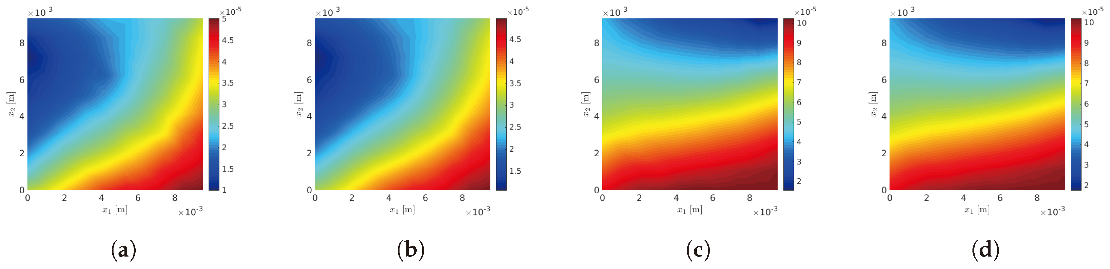
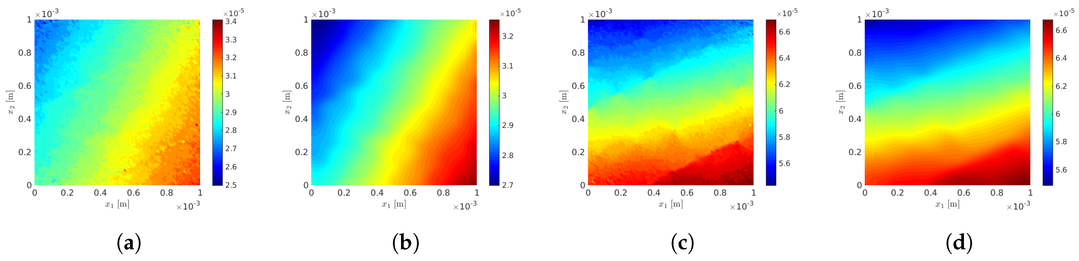
 for the mesoscopic domain of observation . (a) cross-section ; (b) cross-section ; (c) cross-section .
for the mesoscopic domain of observation . (a) cross-section ; (b) cross-section ; (c) cross-section .
for the mesoscopic domain of observation . (a) cross-section ; (b) cross-section ; (c) cross-section .


| [GPa] | [GPa] | |
|---|---|---|
| Relative error [%] |
| ℓ [m] | [GPa] | [GPa] | |||
|---|---|---|---|---|---|
| 3 | |||||
| 4 | |||||
| 3 | |||||
| 3 | |||||
| 3 | |||||
| 4 | |||||
| 4 | |||||
| 4 | |||||
| 3 | |||||
| 4 | |||||
| 4 | |||||
| 3 | |||||
| 4 | |||||
| 3 | |||||
| 4 | |||||
| 4 | |||||
| - | |||||
| - | |||||
| Relative error [%] | - | ||||
| 855,000 | |||||
| ℓ [m] | [GPa] | [GPa] | |||
|---|---|---|---|---|---|
| - | |||||
| () | 855,000 | ||||
| Relative error [%] | - | ||||
| () | 87,000 | ||||
| Relative error [%] | - | ||||
| () | 9000 | ||||
| Relative error [%] | - |
| ℓ [m] | [GPa] | [GPa] | |||
|---|---|---|---|---|---|
| 193 | |||||
| 202 | |||||
| 189 | |||||
| 197 | |||||
| 207 | |||||
| 201 | |||||
| 192 | |||||
| 199 | |||||
| 210 | |||||
| 205 | |||||
| 203 | |||||
| 198 | |||||
| 194 | |||||
| 208 | |||||
| 190 | |||||
| 208 | |||||
| - | |||||
| - | |||||
| Relative error [%] | - | ||||
| 19,176,000 | |||||
| [GPa] | [GPa] | |
|---|---|---|
| Relative error [%] |
| ℓ [m] | [GPa] | [GPa] | |||
|---|---|---|---|---|---|
| 3 | |||||
| 4 | |||||
| 3 | |||||
| - | |||||
| - | |||||
| Relative error [%] | - | ||||
| 150,000 | |||||
| [GPa] | [GPa] | |
|---|---|---|
| ℓ [m] | [GPa] | [GPa] | |||
|---|---|---|---|---|---|
| 5 | |||||
| 7500 | |||||
© 2020 by the authors. Licensee MDPI, Basel, Switzerland. This article is an open access article distributed under the terms and conditions of the Creative Commons Attribution (CC BY) license (http://creativecommons.org/licenses/by/4.0/).
Share and Cite
Zhang, T.; Pled, F.; Desceliers, C. Robust Multiscale Identification of Apparent Elastic Properties at Mesoscale for Random Heterogeneous Materials with Multiscale Field Measurements. Materials 2020, 13, 2826. https://doi.org/10.3390/ma13122826
Zhang T, Pled F, Desceliers C. Robust Multiscale Identification of Apparent Elastic Properties at Mesoscale for Random Heterogeneous Materials with Multiscale Field Measurements. Materials. 2020; 13(12):2826. https://doi.org/10.3390/ma13122826
Chicago/Turabian StyleZhang, Tianyu, Florent Pled, and Christophe Desceliers. 2020. "Robust Multiscale Identification of Apparent Elastic Properties at Mesoscale for Random Heterogeneous Materials with Multiscale Field Measurements" Materials 13, no. 12: 2826. https://doi.org/10.3390/ma13122826
APA StyleZhang, T., Pled, F., & Desceliers, C. (2020). Robust Multiscale Identification of Apparent Elastic Properties at Mesoscale for Random Heterogeneous Materials with Multiscale Field Measurements. Materials, 13(12), 2826. https://doi.org/10.3390/ma13122826