Efficient Toughening of Short-Fiber Composites Using Weak Magnetic Fields


Abstract

1. Introduction
2. Experimental
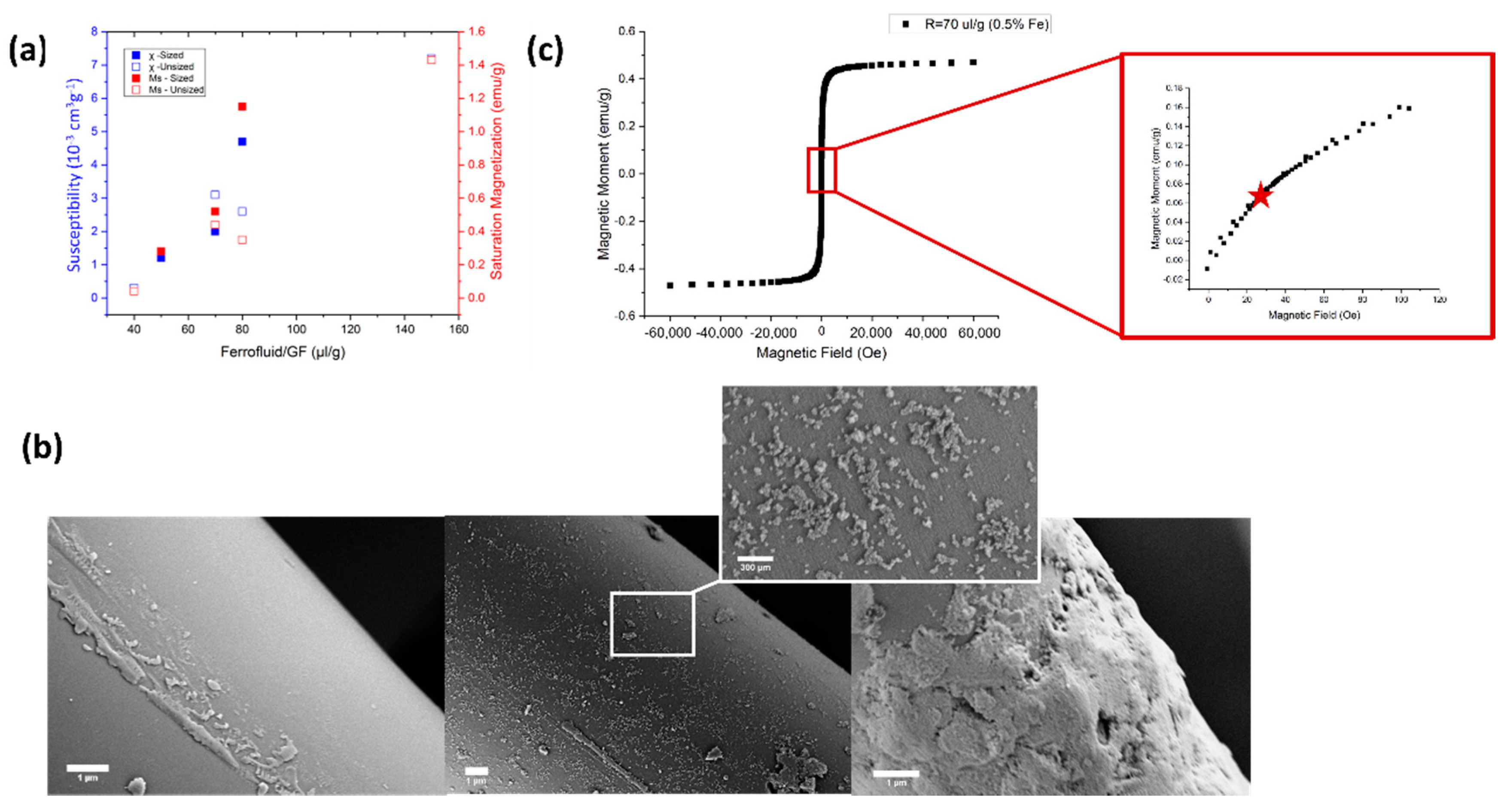
2.1. Magnetization of Glass Fibers
2.2. Composite Preparation
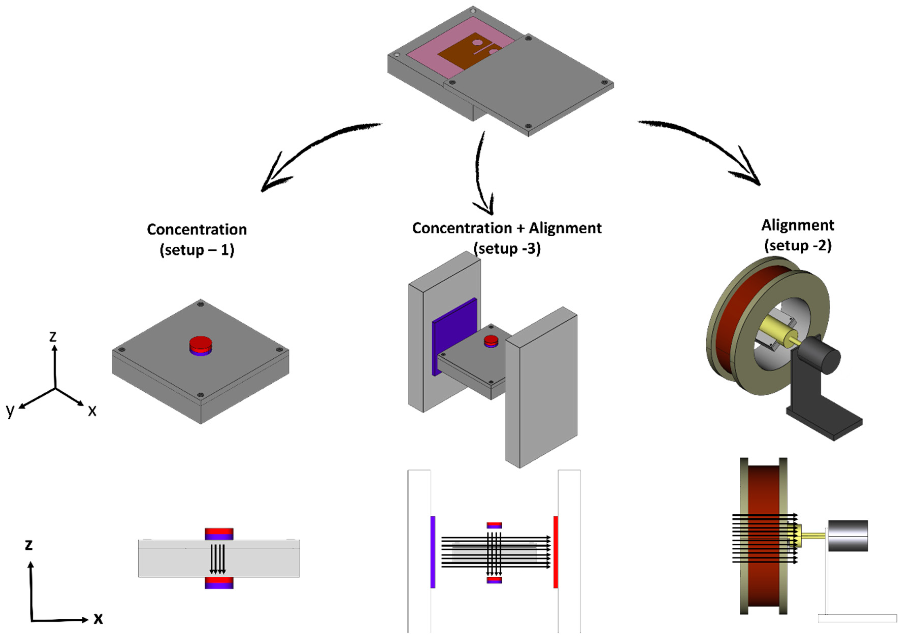
2.3. Curing Protocol and Setup
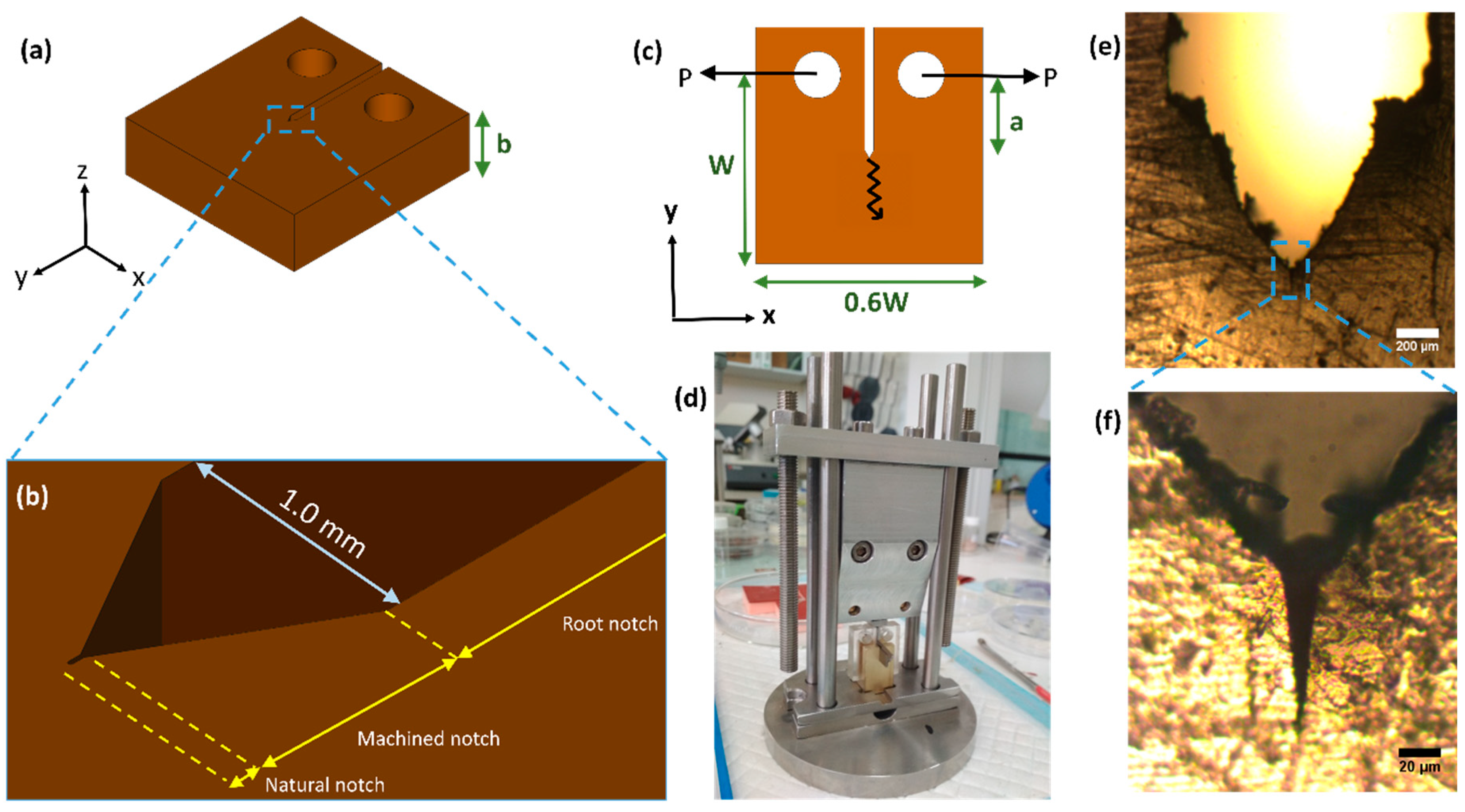
2.4. Notching
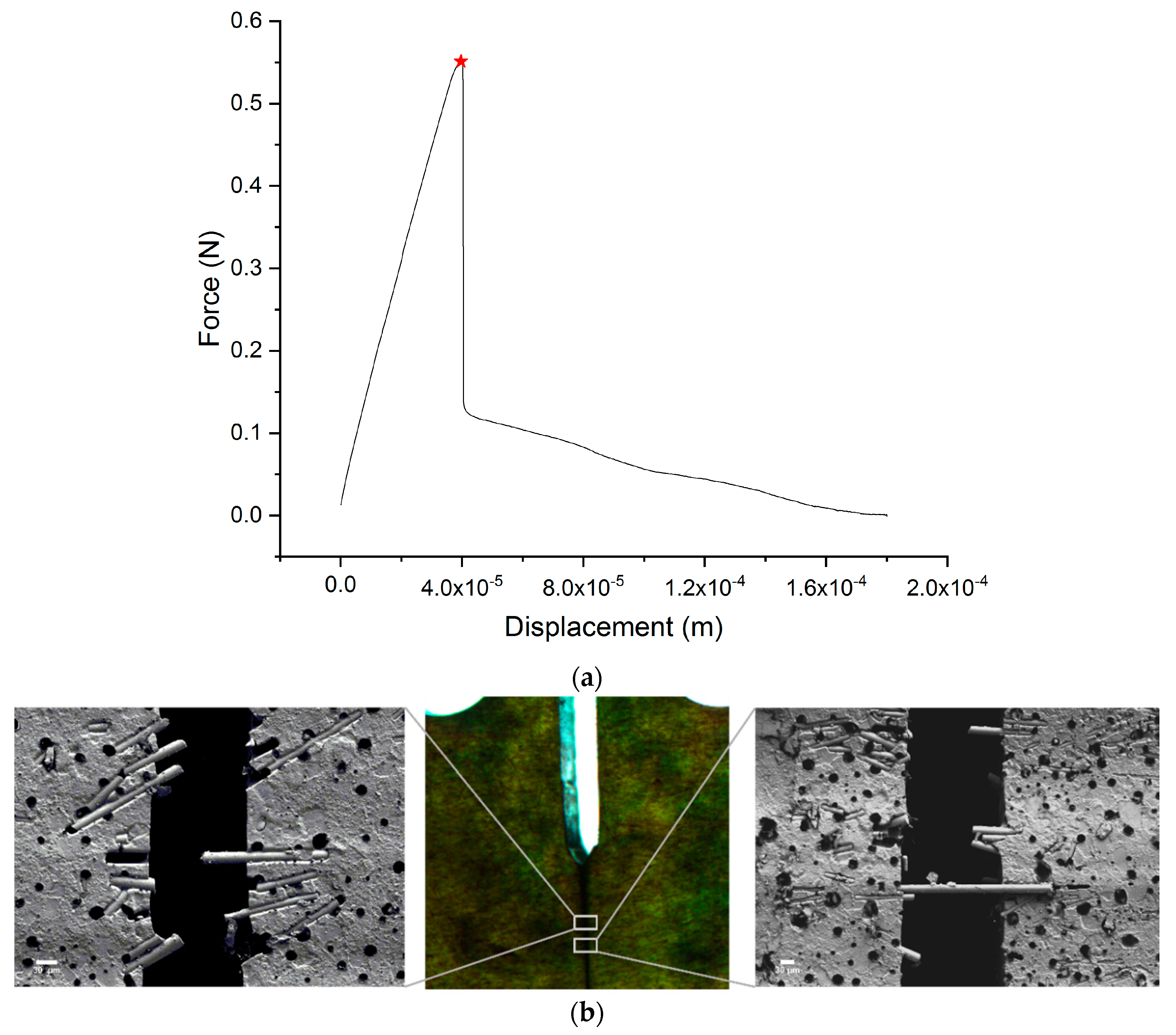
2.5. Mechanical Testing
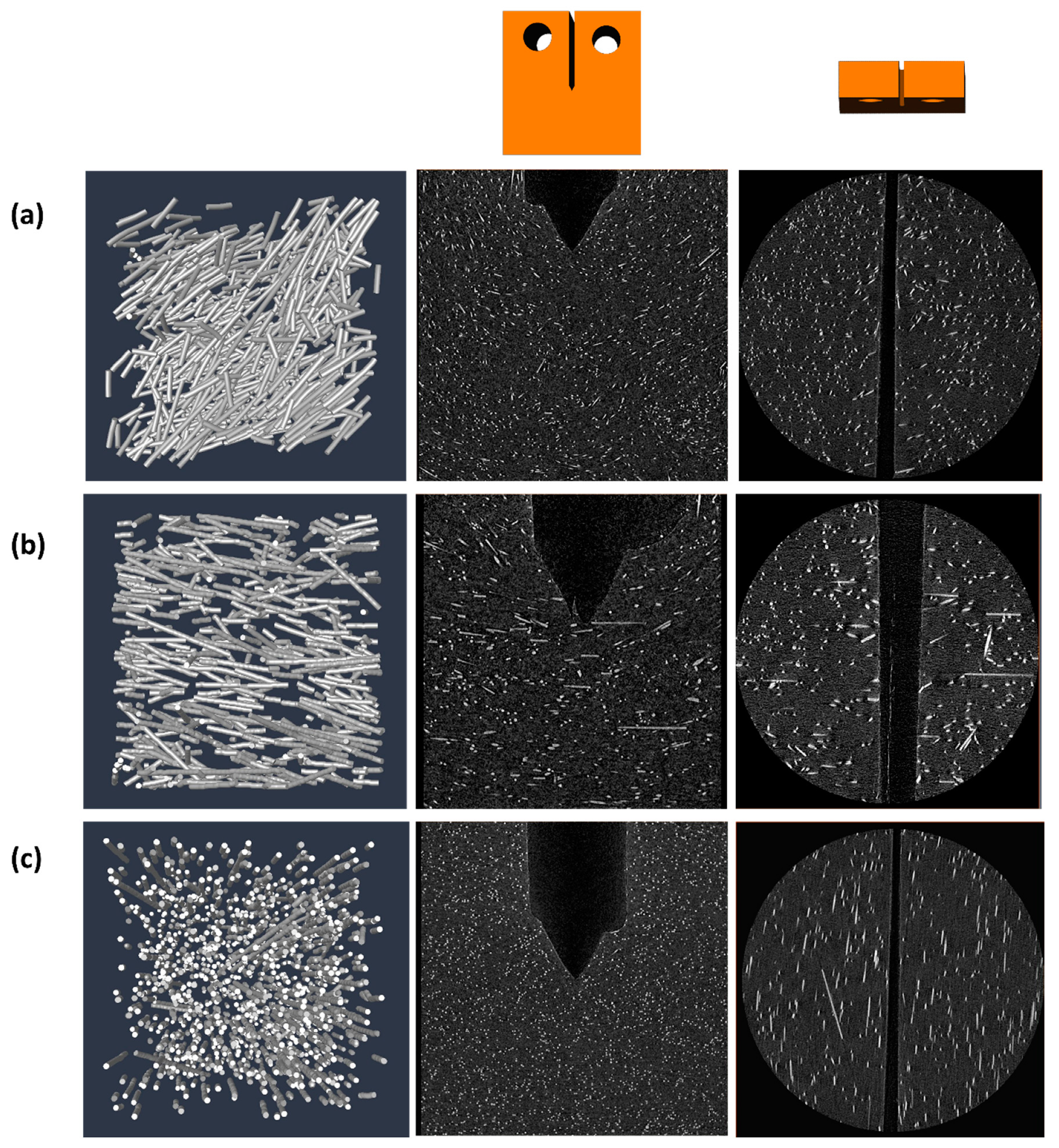
2.6. Imaging
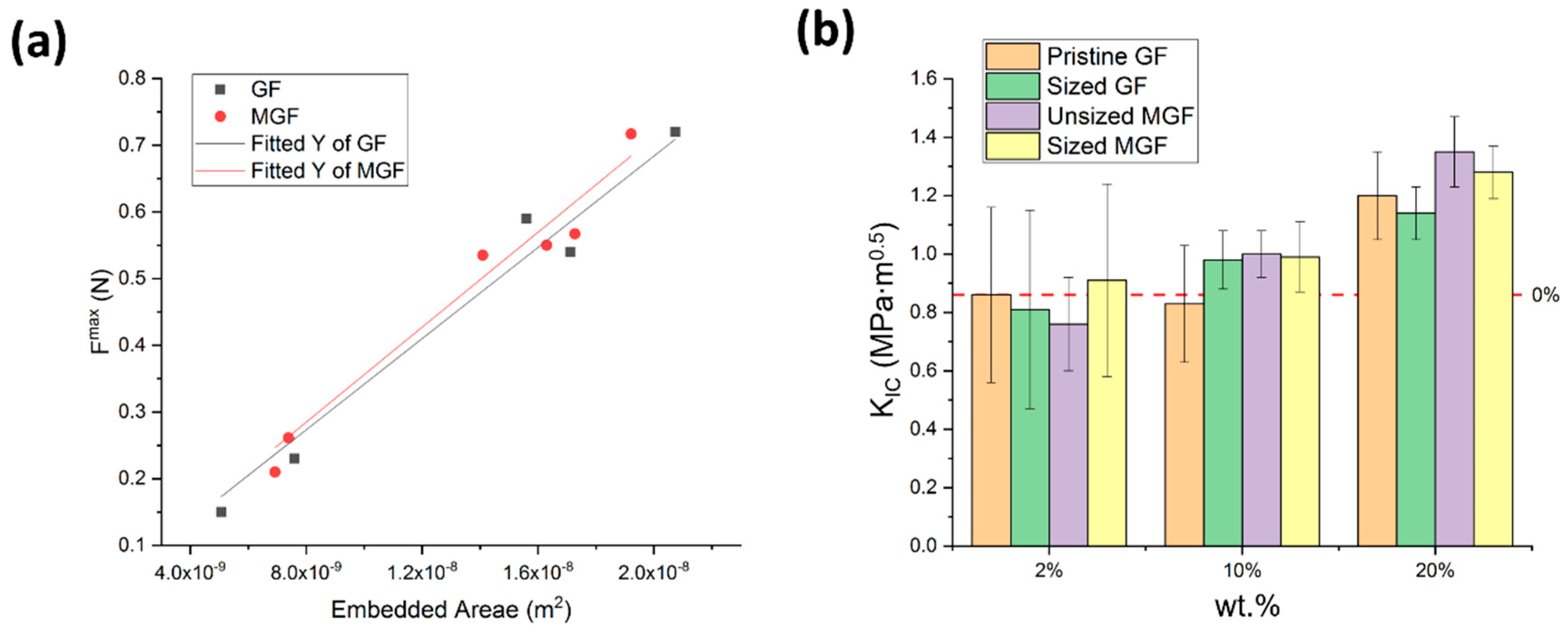
2.7. Micromechanics
3. Results and Discussion
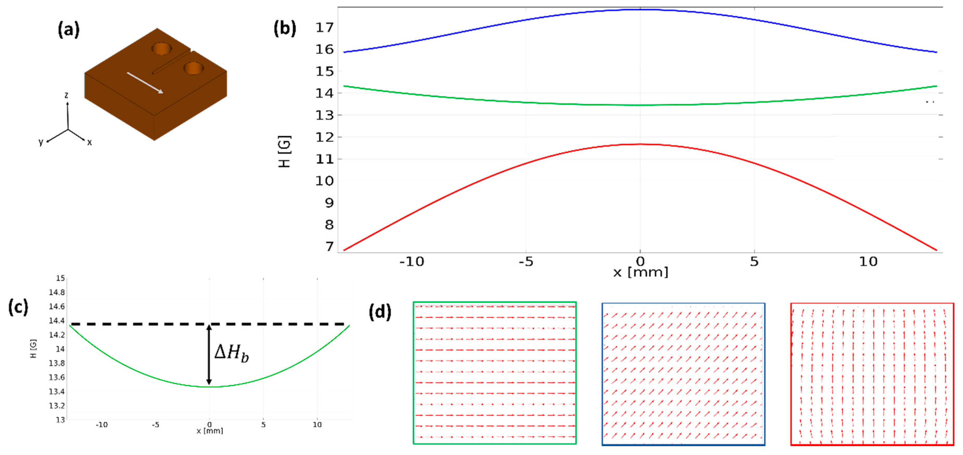
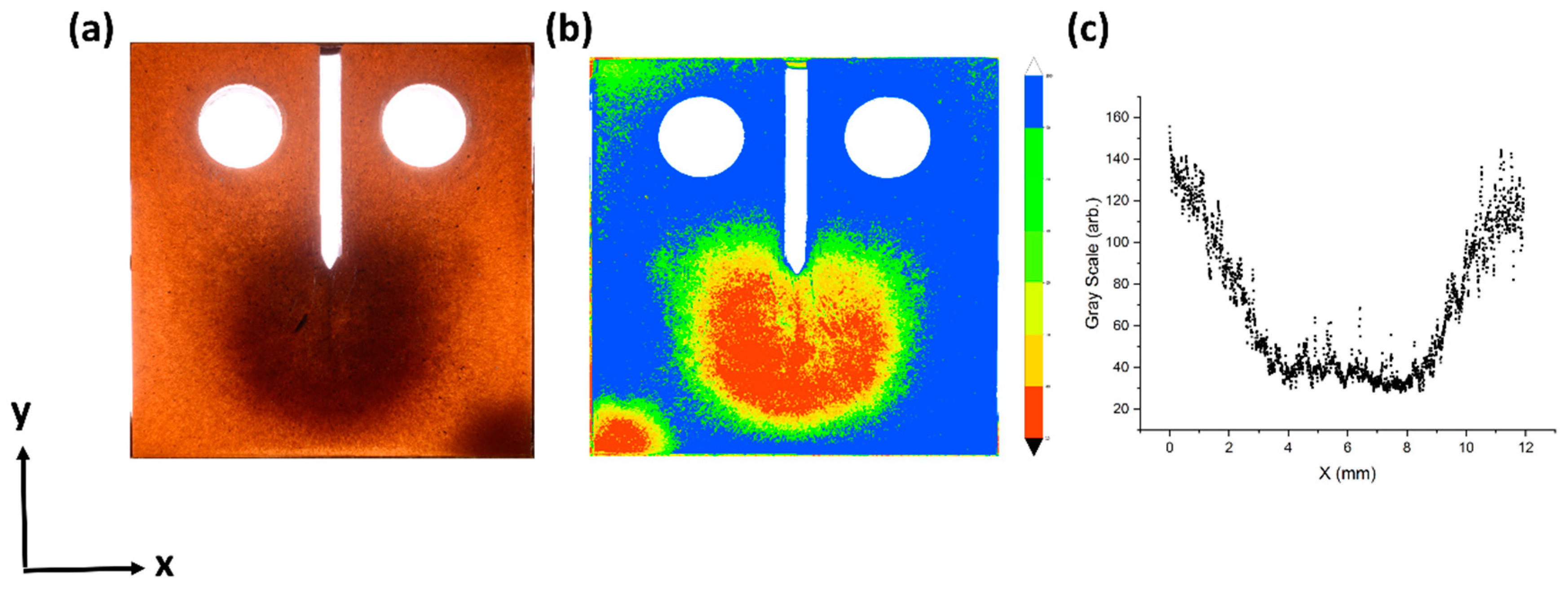
3.1. System Characterization
3.2. Magnetic Translation and Rotation
3.3. Mechanical Analysis
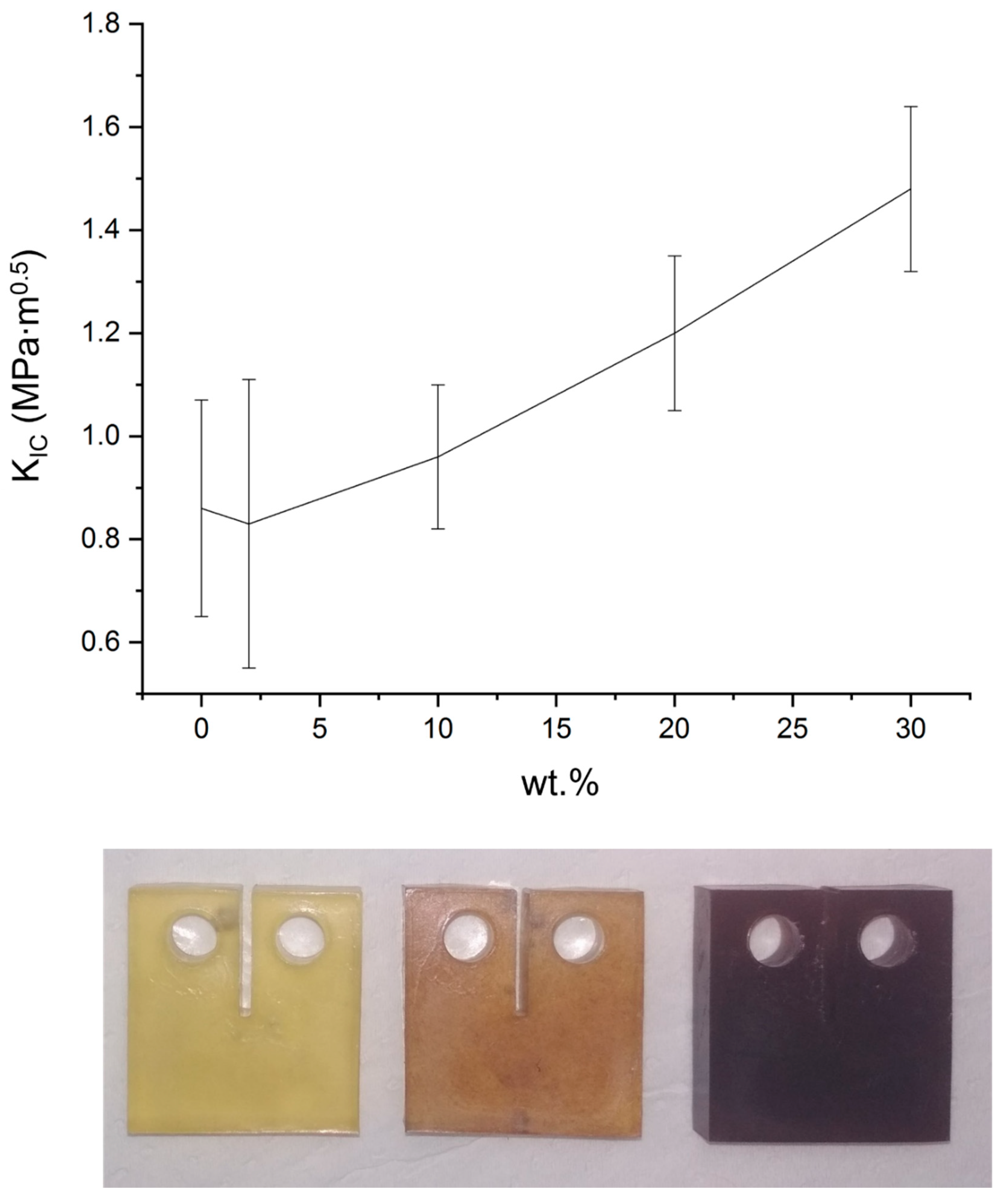
3.4. Mechanical Measurements
3.5. Toughening Mechanisms
4. Summary and Conclusions
Supplementary Materials
Author Contributions
Funding
Acknowledgments
Conflicts of Interest
References
- Hashin, Z. Analysis of Composite Materials—A Survey. J. Appl. Mech. 1983, 50, 481. [Google Scholar] [CrossRef]
- Zhang, W. Technical Problem Identification for the Failures of the Liberty Ships. Challenges 2016, 7, 20. [Google Scholar] [CrossRef]
- Griffith, A. The Phenomena of Rupture and Flow in Solid. In Philosophical Transactions of the Royal Society of London. Series A, Containing Papers of A Mathematical or Physical Character; The Royal Society: London, UK, 1921; pp. 163–198. [Google Scholar]
- Malek, A.M.; Saadatmanesh, H.; Ehsani, M.R. Prediction of failure load of R/C beams strengthened with FRP plate due to stress concentration at the plate end. ACI Struct. J. 1998, 95, 142–152. [Google Scholar]
- Livieri, P.; Lazzarin, P. Fatigue strength of steel and aluminium welded joints based on generalised stress intensity factors and local strain energy values. Int. J. Fract. 2005, 133, 247–276. [Google Scholar] [CrossRef]
- Ritchie, R.O. The conflicts between strength and toughness. Nat. Mater. 2011, 10, 817–822. [Google Scholar] [CrossRef] [PubMed]
- Marston, T.U.; Atkins, A.G.; Felbeck, D.K. Interfacial fracture energy and the toughness of composites. J. Mater. Sci. 1974, 9, 447–455. [Google Scholar] [CrossRef]
- Fu, S.Y.; Lauke, B. The fibre pull-out energy of misaligned short fibre composites. J. Mater. Sci. 1997, 32, 1985–1993. [Google Scholar] [CrossRef]
- Mai, Y.-W.; Lauke, B. Fracture Mechanics. In Science and Engineering of Short Fibre Reinforced Polymer Composites; Woodhead Publishing: Sawston, UK, 2009; pp. 231–331. [Google Scholar]
- Wetherhold, R.C.; Jain, L.K. The effect of crack orientation on the fracture properties of composite materials. Mater. Sci. Eng. A 1993, 165, 91–97. [Google Scholar] [CrossRef]
- Fu, S.Y.; Lauke, B. Effects of fiber length and fiber orientation distributions on the tensile strength of short-fiber-reinforced polymers. Compos. Sci. Technol. 1996, 56, 1179–1790. [Google Scholar] [CrossRef]
- Greenfeld, I.; Wagner, H.D. Nanocomposite toughness, strength and stiffness: Role of filler geometry. Nanocomposites 2015, 1, 3–17. [Google Scholar] [CrossRef][Green Version]
- Anderson, T.L. Fracture Mechanics: Fundamentals and Applications, 2nd ed.; Taylor & Francis Group: Boca Raton, FL, USA, 1994. [Google Scholar]
- Goldberg, O.; Greenfeld, I.; Wagner, H.D. Composite Reinforcement by Magnetic Control of Fiber Density and Orientation. ACS Appl. Mater. Interfaces 2018, 10, 16802–16811. [Google Scholar] [CrossRef] [PubMed]
- Wang, X.; Zhao, Z.; Qu, J.; Wang, Z.; Qiu, J. Fabrication and Characterization of Magnetic Fe3O4-CNT Composites. J. Phys. Chem. Solids 2010, 71, 673–676. [Google Scholar] [CrossRef]
- Laurent, S.; Forge, D.; Port, M.; Roch, A.; Robic, C.; Vander, E.L.; Muller, R.N. Magnetic Iron oxide Nanoparticles: Synthesis, Stabilization, Vectorization, Physicochemical Characterizations and Biological Applications. Chem. Rev. 2008, 108, 2064–2110. [Google Scholar] [CrossRef]
- Frogley, M.D.; Wagner, H.D. Mechanical Alignment of Quasi-One-Dimensional Nanoparticles. J. Nanosci. Nanotechnol. 2002, 2, 517–521. [Google Scholar] [CrossRef] [PubMed]
- Erb, R.M.; Libanori, R.; Rothfuchs, N.; Studart, A.R. Composites Reinforced in Three Dimensions by Using Low Magnetic Fields. Science 2012, 335, 199–204. [Google Scholar] [CrossRef] [PubMed]
- Ravindran, A.R.; Ladani, R.B.; Wu, S.; Kinloch, A.J.; Wang, C.H.; Mouritz, A.P. The electric field alignment of short carbon fibres to enhance the toughness of epoxy composites. Compos. Part A Appl. Sci. Manuf. 2018, 106, 11–23. [Google Scholar] [CrossRef]
- Ma, C.; Liu, H.-Y.; Du, X.; Mach, L.; Xu, F.; Mai, Y.-W. Fracture resistance, thermal and electrical properties of epoxy composites containing aligned carbon nanotubes by low magnetic field. Compos. Sci. Technol. 2015, 114, 126–135. [Google Scholar] [CrossRef]
- Lachman, N.; Wagner, H.D. Correlation between interfacial molecular structure and mechanics in CNT/epoxy nano-composites. Compos. Part A Appl. Sci. Manuf. 2010, 41, 1093–1098. [Google Scholar] [CrossRef]
- Erb, R.M.; Martin, J.J.; Soheilian, R.; Pan, C.; Barber, J.R. Actuating Soft Matter with Magnetic Torque. Adv. Funct. Mater. 2016, 26, 3859–3880. [Google Scholar] [CrossRef]
- Kimura, T. Study on the Effect of Magnetic Fields on Polymeric Materials and Its Application. Polym. J. 2003, 35, 823–843. [Google Scholar] [CrossRef]
- Camponeschi, E.; Vance, R.; Al-Haik, M.; Garmestani, H.; Tannenbaum, R. Properties of carbon nanotube-polymer composites aligned in a magnetic field. Carbon 2007, 45, 2037–2046. [Google Scholar] [CrossRef]
- Wu, S.; Ladani, R.B.; Zhang, J.; Kinloch, A.J.; Zhao, Z.; Ma, J.; Zhang, X.H.; Adrian, P.M.; Kamra, G.; Chun, H.; et al. Epoxy nanocomposites containing magnetite-carbon nanofibers aligned using a weak magnetic field. Polymer 2015, 68, 25–34. [Google Scholar] [CrossRef]
- Prolongo, S.G.; Meliton, B.G.; Del, R.G.; Ureña, A. New Alignment Procedure of Magnetite-CNT Hybrid Nanofillers on Epoxy Bulk Resin with Permanent Magnets. Compos. Part B Eng. 2013, 46, 166–172. [Google Scholar] [CrossRef]
- Martin, J.J.; Fiore, B.E.; Erb, R.M. Designing Bioinspired Composite Reinforcement Architectures via 3D Magnetic Printing. Nat. Commun. 2015, 6, 1–7. [Google Scholar] [CrossRef]
- Le, F.H.; Bouville, F.; Niebel, T.P.; Studart, A.R. Magnetically Assisted Slip Casting of Bioinspired Heterogeneous Composites. Nat. Mater. 2015, 14, 1–17. [Google Scholar]
- Bargardi, F.L.; Le, F.H.; Libanori, R.; Studart, A.R. Bio-inspired self-shaping ceramics. Nat. Commun. 2016, 7, 1–8. [Google Scholar] [CrossRef]
- Schmied, J.U.; Le, F.H.; Ermanni, P.; Studart, A.R.; Arrieta, A.F. Programmable snapping composites with bio-inspired architecture. Bioinspir. Biomim. 2017, 12, 026012. [Google Scholar] [CrossRef]
- Erb, R.M.; Segmehl, J.; Charilaou, M.; Löffler, J.F.; Studart, A.R. Non-linear Alignment Dynamics in Suspensions of Platelets under Rotating Magnetic Fields. Soft Matter 2012, 8, 7604–7609. [Google Scholar] [CrossRef]
- Standard Test Methods for Plane-Strain Fracture Toughness and Strain Energy Release Rate of Plastic Materials; ASTM Standard D5045-99; ASTM International: West Conshohocken, PA, USA, 1999.
- Moore, D.R. The measurement of Kc and Gc at slow speeds for discontinuous fibre composites. Eur. Struct. Integr. Soc. 2001, 28, 59–72. [Google Scholar]
- Norman, D.A.; Robertson, R.E. The effect of fiber orientation on the toughening of short fiber-reinforced polymers. J. Appl. Polym. Sci. 2003, 90, 2740–2751. [Google Scholar] [CrossRef]
- Ibrahim, R.N.; Stark, H.L. Validity requirements for fracture toughness measurements obtained from small circumferentially notched cylindrical specimens. Eng. Fract. Mech. 1987, 28, 455–460. [Google Scholar] [CrossRef]
- Mower, T.M.; Li, V.C. Fracture characterization of random short fiber reinforced thermoset resin composites. Eng. Fract. Mech. 1987, 26, 593–603. [Google Scholar] [CrossRef]
- Krenchel, H. Fibre Reinforcement: Theoretical and Practical Investigations of the Elasticity and Strength of Fibre-reinforced Materials; Akademisk Forlag: Copenhagen, Danmark, 1964. [Google Scholar]
- Wang, Y.; Lf, V.C.; Backer, S. Modelling of fibre pull-out from a cement matrix. Int. J. Cem. Compos. Light Concr. 1988, 10, 143–149. [Google Scholar] [CrossRef]
- Brandt, A.M. On the optimal direction of short metal fibres in brittle matrix composites. J. Mater. Sci. 1985, 20, 3831–3841. [Google Scholar] [CrossRef]
- Kim, J.-K.; Mai, Y.-W. High Strength, High Fracture Toughness Fibre Composites with Interface Control-A Review. Compos. Sci. Technol. 1991, 41, 333–378. [Google Scholar] [CrossRef]
- Hull, D.; Clyne, T. An Introduction to Composite Materials; Cambridge University Press: Cambridge, UK, 1996; pp. 43–53. [Google Scholar]
- Piggott, M.R. Load Bearing Fibre Composites, 2nd ed.; Kluwer Academic Publishers: Berlin, Germany, 2002. [Google Scholar]
- Fratzl, P.; Gupta, H.S.; Fischer, F.D.; Kolednik, O. Hindered crack propagation in materials with periodically varying young’s modulus-Lessons from biological materials. Adv. Mater. 2007, 19, 2657–2661. [Google Scholar] [CrossRef]
- Mirkhalaf, M.; Dastjerdia, K.; Barthelat, F. Overcoming the brittleness of glass through bio-inspiration and micro-architecture. Nat. Commun. 2014, 5, 3166. [Google Scholar] [CrossRef]
- Malik, I.A.; Barthelat, F. Toughening of thin ceramic plates using bioinspired surface patterns. Int. J. Solids Struct. 2016, 97, 1–11. [Google Scholar] [CrossRef]
- Kolednik, O. The yield stress gradient effect in inhomogenous materials. Int. J. Solids Struct. 2000, 37, 781–808. [Google Scholar] [CrossRef]


| Sample | Description (see Figure 2) | Orientation (see Figure 6) | Concentration | Hc/Hb |
|---|---|---|---|---|
| Control | None | Random | Uniform | - |
| Setup 1 | A pair of small permanent magnets | Unidirectional (Z) | Concentrated near the crack-tip | ∞ |
| Setup 2 | Solenoid and rotated motor | Unidirectional (X) | Uniform | 0 |
| Setup 3 | A pair of small permanent magnets + Bias magnetic field | Unidirectional (X) | Concentrated near the crack-tip | > 0 |
| wt % | KIC [MPa·m0.5] | KIC/KIC,0 |
|---|---|---|
| 0 | 0.86 ± 0.21 | 1.00 |
| 2 | 0.83 ± 0.28 | 0.97 |
| 10 | 0.96 ± 0.14 | 1.12 |
| 20 | 1.20 ± 0.15 | 1.40 |
| 30 | 1.48 ± 0.16 | 1.72 |
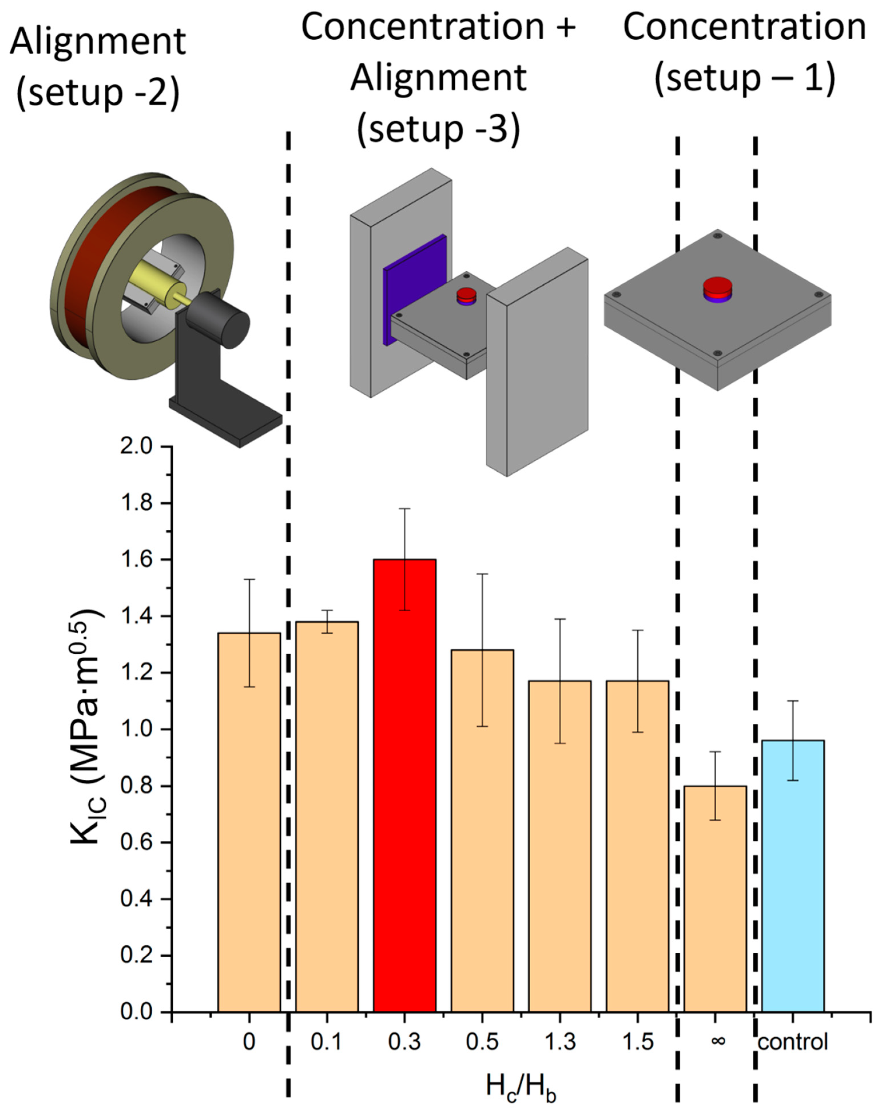
| Hc/Hb [G/G] | KIC [MPa·m0.5] | KIC/KIC,0 | |
|---|---|---|---|
| 0 (solenoid) | 0 | 1.34 ± 0.19 | 1.56 |
| 0.1 | 0.6 | 1.38 ± 0.04 | 1.60 |
| 0.3 | 5 | 1.60 ± 0.18 | 1.86 |
| 0.5 | 14 | 1.28 ± 0.27 | 1.49 |
| 1.3 | 59 | 1.17 ± 0.22 | 1.36 |
| 1.5 | 66 | 1.17 ± 0.18 | 1.36 |
| ∞ (no bias) | 90 | 0.80 ± 0.12 | 0.93 |
| control | 38 | 0.96 ± 0.14 | 1.12 |
| Symbol | Description | Method | Value | Units |
|---|---|---|---|---|
| df | Short fiber diameter | SEM | 16 | μm |
| lf | Short fiber average length | μCT | 220 ± 50 | μm |
| Em | Matrix tensile modulus | Tensile (dog-bone) | 1.22 ± 0.14 | GPa |
| Ef | Fiber tensile modulus | Tensile | 80 ± 12 | GPa |
| σy0 | Matrix yield stress | Tensile (dog-bone) | 72.6 ± 4.1 | MPa |
| σmmax0 | Matrix ultimate stress | Tensile (dog-bone) | 100.8 ± 0.14 | MPa |
| σf | Fiber ultimate strength | Tensile (Weibull) | 3248 ± 50 | MPa |
| τi | Interfacial shear strength | Pull-out | 34.6 ± 2.9 | MPa |
| Gi | fiber-matrix surface energy | Pull-out | 1.6 ± 0.8 | kJ/m2 |
| lc | Critical length | Calculated [42] | 740 | μm |
| rp | Radius of plasticity | Calculated [13] | 28 | μm |
| Dpz | Process-zone size | Calculated [34] | 650 | μm |
© 2020 by the authors. Licensee MDPI, Basel, Switzerland. This article is an open access article distributed under the terms and conditions of the Creative Commons Attribution (CC BY) license (http://creativecommons.org/licenses/by/4.0/).
Share and Cite
Goldberg, O.; Greenfeld, I.; Wagner, H.D. Efficient Toughening of Short-Fiber Composites Using Weak Magnetic Fields. Materials 2020, 13, 2415. https://doi.org/10.3390/ma13102415
Goldberg O, Greenfeld I, Wagner HD. Efficient Toughening of Short-Fiber Composites Using Weak Magnetic Fields. Materials. 2020; 13(10):2415. https://doi.org/10.3390/ma13102415
Chicago/Turabian StyleGoldberg, Omri, Israel Greenfeld, and Hanoch Daniel Wagner. 2020. "Efficient Toughening of Short-Fiber Composites Using Weak Magnetic Fields" Materials 13, no. 10: 2415. https://doi.org/10.3390/ma13102415
APA StyleGoldberg, O., Greenfeld, I., & Wagner, H. D. (2020). Efficient Toughening of Short-Fiber Composites Using Weak Magnetic Fields. Materials, 13(10), 2415. https://doi.org/10.3390/ma13102415