Mathematical Modeling of Breast Tumor Destruction Using Fast Heating during Radiofrequency Ablation


Abstract
1. Introduction
2. Materials and Methods
2.1. Introduction
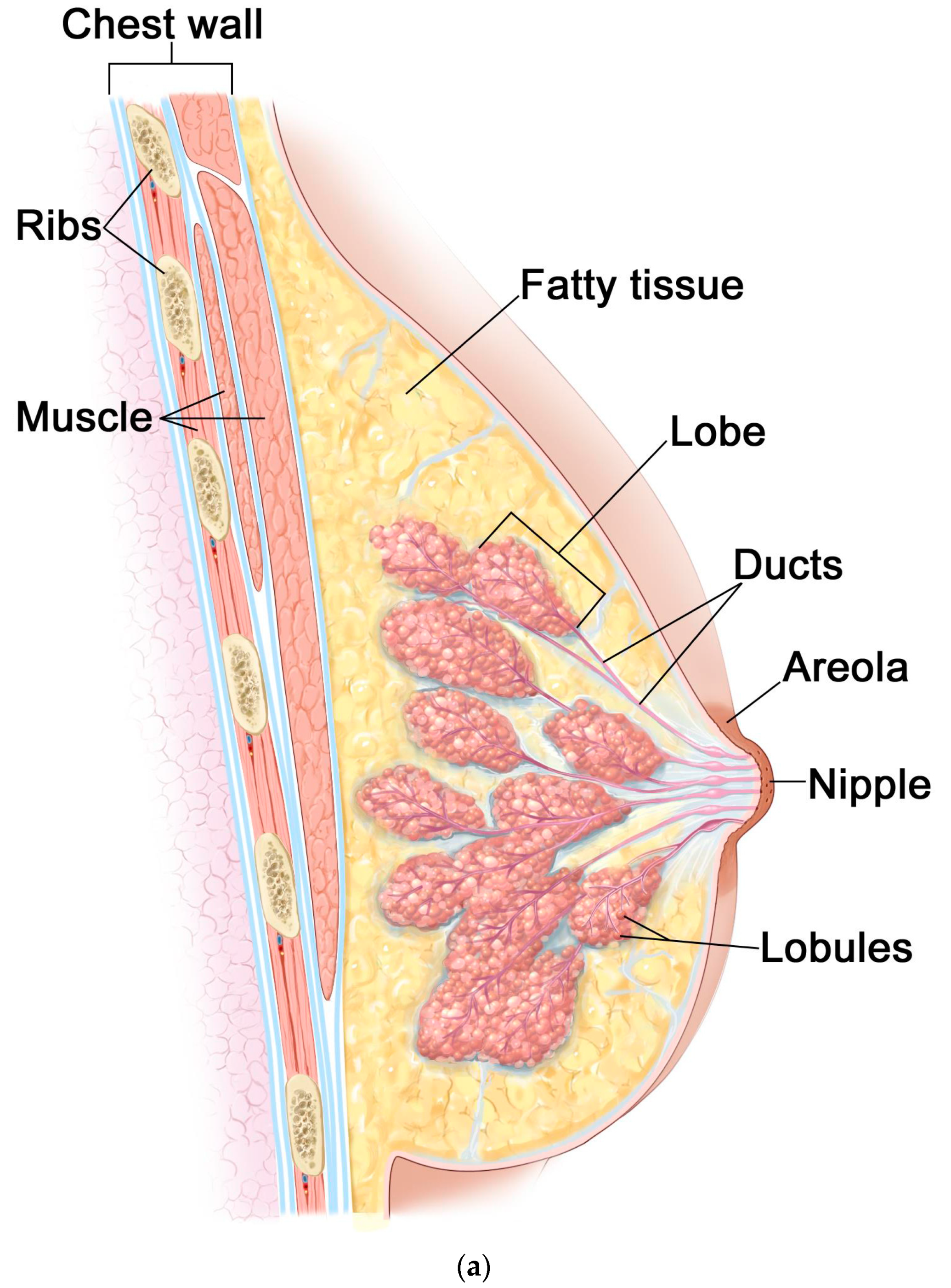
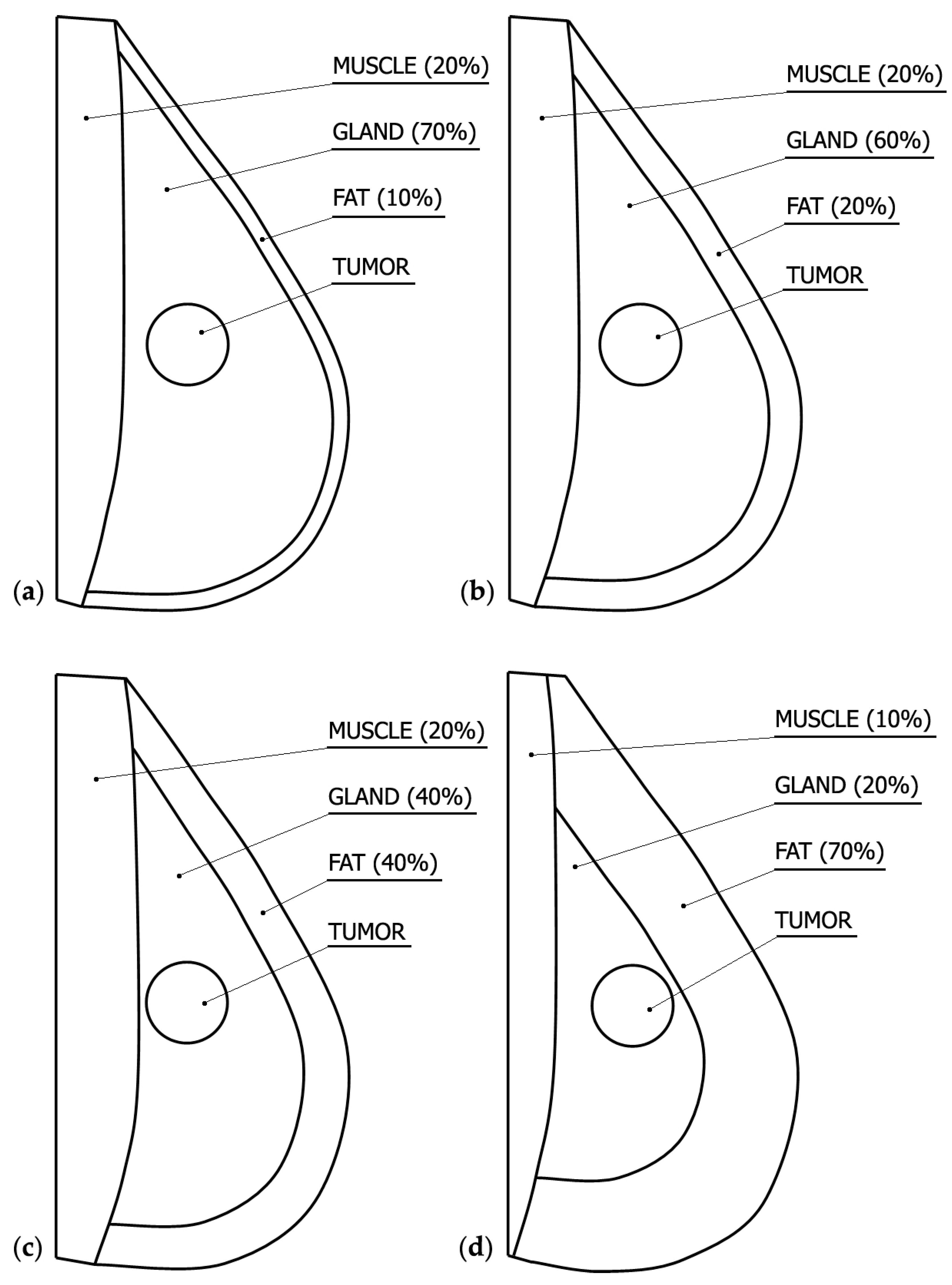
2.2. Breast Modeling
2.3. Mathematical Modeling of Electric and Temperature Fields
- the initial temperature of the electrode tine and trocar domains (indicated as Ω5 and Ω6) have been set to 25 °C, simulating the ambient room temperature condition
- the initial temperature of the breast and tumor domains (indicated as Ω1, Ω2, Ω3 and Ω4) have been considered to be uniform and the same as the body core temperature of the human body
2.4. Arrhenius Scheme—A Model of Tissue Destruction
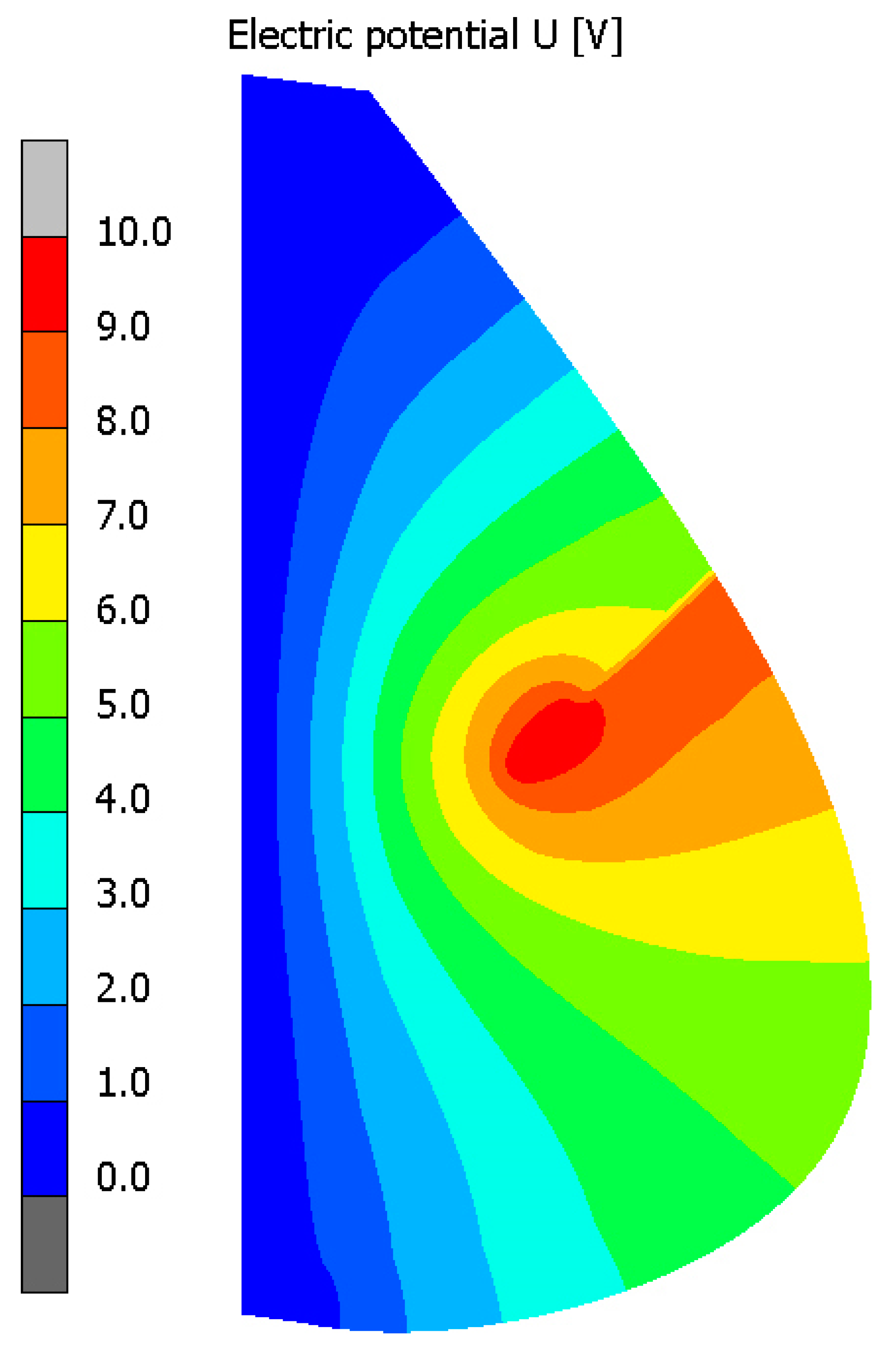
3. Results
4. Discussion
Funding
Conflicts of Interest
References
- Bojakowska, U.; Kalinowski, P.; Kowalska, M.E. Epidemiology and prophylaxis of breast cancer. J. Edu. Health Sport 2016, 6, 701–710. [Google Scholar]
- Lokuhetty, D.; White, V.A.; Watanabe, R.; Cree, I.A.; International Agency for Research on Cancer (IARC). WHO Classification of Tumours. Breast Tumours, 5th ed.; WHO Classification of Tumours Editorial Board; World Health Organization: Genève, Switzerland, 2019. [Google Scholar]
- Wojciechowska, U.; Didkowska, J.; Morbidity and Deaths from Malignant Tumors in Poland. National Cancer Registry, Maria Skłodowska-Curie Institute of Oncology. Available online: http://onkologia.org.pl/rak-piersi-kobiet/ (accessed on 17 June 2019). (In Polish).
- Didkowska, J.; Wojciechowska, U. Breast cancer in Poland and Europe—Population and statistics. J. Oncol. 2013, 63, 111–118. [Google Scholar]
- Ferlay, J.; Shin, H.; Bray, F.; Forman, D.; Mathers, C.; Parkin, D.M. Estimates of worldwide burden of cancer in 2008: GLOBOCAN 2008. Int. J. Cancer 2010, 127, 2893–2917. [Google Scholar] [CrossRef] [PubMed]
- Chu, K.F.; Dupuy, D.E. Thermal ablation of tumours: Biological mechanisms and advances in therapy. Nat. Rev. Cancer 2014, 14, 199–208. [Google Scholar] [CrossRef]
- Zhao, Z.; Wu, F. Minimally-invasive thermal ablation of early-stage breast cancer: A systemic review. EJSO-Eur. J. Surg. Oncol. 2010, 36, 1149–1155. [Google Scholar] [CrossRef]
- Sundeep, S.; Repaka, R. Parametric sensitivity analysis of critical factors affecting the thermal damage during RFA of breast tumor. Int. J. Therm. Sci. 2018, 124, 366–374. [Google Scholar]
- Rzepka, E.; Püsküllüoglu, M. The role of hyperthermia in oncological treatment. Oncol. Clin. Pract. 2012, 8, 178–188. [Google Scholar]
- Pennes, H.H. Analysis of tissue and arterial blood temperature in the resting human forearm. J. Appl. Physiol. 1948, 1, 93–122. [Google Scholar] [CrossRef]
- Jamil, M.; Ng, E.Y.K. To optimize the efficacy of bioheat transfer in capacitive hyperthermia: A physical perspective. J. Therm. Biol. 2013, 38, 272–279. [Google Scholar] [CrossRef]
- Lv, Y.G.; Deng, Z.S.; Liu, J. 3D numerical study on the induced heating effects of embedded micro/nanoparticles on human body subject to external medical electromagnetic field. IEEE Trans. Nanobiosci. 2005, 4, 284–294. [Google Scholar]
- Schutt, D.; Berjano, E.J.; Haemmerich, D. Effect of electrode thermal conductivity in cardiac radiofrequency catheter ablation: A computational modeling study. Int. J. Hyperther. 2009, 25, 99–107. [Google Scholar] [CrossRef]
- Majchrzak, E.; Mochnacki, B.; Dziewonski, M.; Jasinski, M. Numerical modelling of hyperthermia and hypothermia processes. In Advanced Materials Research, Proceedings of the International Conference on Computational Materials Science (CMS 2011), Guangzhou, China, 17–18 April 2011; Xiong, F., Ed.; Trans Tech Publications: Guangzhou, China, 2011; pp. 268–270. [Google Scholar]
- Gasselhuber, A.; Dreher, M.R.; Negussie, A.; Wood, B.J.; Rattay, F.; Haemmerich, D. Mathematical spatio-temporal model of drug delivery from low temperature sensitive liposomes during radiofrequency tumour ablation. Int. J. Hyperther. 2010, 26, 499–513. [Google Scholar] [CrossRef]
- Paruch, M. Cancer ablation during RF hyperthermia using internal electrode. In Advances in Mechanics: Theoretical, Computational and Interdisciplinary Issues, 1st ed.; Kleiber, M., Burczynski, T., Wilde, K., Gorski, J., Winkelmann, K., Smakosz, L., Eds.; Taylor&Francis Group, CRC Press: Boca Raton, FL, USA, 2016; pp. 455–458. [Google Scholar]
- Andreuccetti, D.; Zoppetti, N. Quasi-static electromagnetic dosimetry: From basic principles to examples of applications. Int. J. Occup. Saf. Ergon. 2006, 12, 201–215. [Google Scholar] [CrossRef]
- Varon, L.A.B.; Orlande, H.R.B.; Elicabe, G.E. Estimation of state variables in the hyperthermia therapy of cancer with heating imposed by radiofrequency electromagnetic waves. Int. J. Therm. Sci. 2015, 98, 228–236. [Google Scholar] [CrossRef]
- Lamien, B.; Varon, L.A.B.; Orlande, H.R.B.; Elicabe, G.E. State estimation in bioheat transfer: A comparison of particle filter algorithms. Int. J. Numer. Methods Heat Fluid Flow 2017, 27, 615–638. [Google Scholar] [CrossRef]
- Ng, E.Y.K.; Jamil, M. Parametric sensitivity analysis of radiofrequency ablation with efficient experimental design. Int. J. Therm. Sci. 2014, 80, 41–47. [Google Scholar] [CrossRef]
- Paruch, M. Identification of the cancer ablation parameters during RF hyperthermia using gradient, evolutionary and hybrid algorithms. Int. J. Numer. Methods Heat Fluid Flow 2017, 27, 674–697. [Google Scholar] [CrossRef]
- Doss, J.D. Calculation of electric fields in conductive media. Med. Phys. 1982, 9, 566–573. [Google Scholar] [CrossRef]
- Van Sonnenberg, E.; McNullen, W.N.; Solbiati, L. Tumor Ablation. Principles and Practice; Springer: New York, NY, USA, 2005; pp. 3–16. [Google Scholar]
- Goldberg, S.N.; Saldinger, P.F.; Gazelle, G.S.; Huertas, J.C.; Stuart, K.E.; Jacobs, T.; Kruskal, J.B. Percutaneous tumor ablation: Increased necrosis with combined radio-frequency ablation and intratumoral doxorubicin injection in a rat breast tumor model. Radiology 2001, 220, 420–427. [Google Scholar] [CrossRef]
- Hung, K.Y.; Lin, Y.C.; Feng, H.P. The effects of acid etching on the nanomorphological surface characteristics and activation energy of titanium medical materials. Materials 2017, 10, 1164–1177. [Google Scholar] [CrossRef]
- Yiming, L.; Hongchao, J.; Zhongman, C.; Xuefeng, T.; Yaogang, L.; Jinping, L. Comparative study on constitutive models for 21-4N heat resistant steel during high temperature deformation. Materials 2019, 12, 1893–1915. [Google Scholar]
- Siteman Cancer Center. Breast Cancer Treatment. General Information about Breast Cancer. Available online: https://siteman.wustl.edu/ncipdq/cdr0000062955/ (accessed on 16 June 2019).
- Siteman Cancer Center. Breast Cancer Treatment. Stages of Breast Cancer. Available online: https://siteman.wustl.edu/ncipdq/cdr0000062955/ (accessed on 16 June 2019).
- Ng, E.Y.K.; Sudharsan, N.M. An improved three-dimensional direct numerical modelling and thermal analysis of a female breast with tumour. J. Eng. Med. 2001, 215, 25–37. [Google Scholar] [CrossRef]
- Wahab, A.A.; Salim, M.I.M.; Ahamat, M.A.; Manaf, N.A.; Yunus, J.; Lai, K.W. Thermal distribution analysis of three-dimensional tumor-embedded breast models with different breast density compositions. Med. Biol. Eng. Comput. 2016, 54, 1363–1373. [Google Scholar] [CrossRef]
- Cheng, D.K. Fundamentals of Engineering Electromagnetics; Addison-Wesley Publishing Company: Boston, MA, USA, 1993. [Google Scholar]
- Paruch, M.; Turchan, L. Mathematical modelling of the destruction degree of cancer under the influence of a RF hyperthermia. AIP Conf. Proc. 2018, 1922, 1–10. [Google Scholar]
- Paruch, M. Identification of the degree of tumor destruction on the basis of the Arrhenius integral using the evolutionary algorithm. Int. J. Therm. Sci. 2018, 130, 507–517. [Google Scholar] [CrossRef]
- Jasinski, M. Numerical analysis of soft tissue damage process caused by laser action. AIP Conf. Proc. 2018, 1922, 1–10. [Google Scholar]
- Gas, P. Optimization of multi-slot coaxial antennas for microwave thermotherapy based on the S11-parameter analysis. Biocybern. Biomed. Eng. 2017, 37, 78–93. [Google Scholar] [CrossRef]
- Zhang, B.; Moser, M.A.; Zhang, E.M.; Luo, Y.; Zhang, H.; Zhang, W. Study of the relationship between the target tissue necrosis volume and the target tissue size in liver tumours using two-compartment finite element RFA modelling. Int. J. Hyperth. 2014, 30, 593–602. [Google Scholar] [CrossRef]
- Nilsson, A.L. Blood flow, temperature, and heat loss of skin exposed to local radiative and convective cooling. J. Investg. Dermatol. 1987, 88, 586–593. [Google Scholar] [CrossRef]
- Osman, M.M.; Afify, E.M. Thermal modelling of the normal woman’s breast. J. Biomech. Eng. 1984, 106, 123–130. [Google Scholar] [CrossRef]
- Abraham, J.P.; Sparrow, E.M. A thermal-ablation bioheat model including liquid-to-vapor phase change, pressure- and necrosis-dependent perfusion, and moisture-dependent properties. Int. J. Heat Mass Transf. 2007, 50, 2537–2544. [Google Scholar] [CrossRef]
- Henriques, F.C. Studies of thermal injuries, V. The predictability and the significance of thermally induced rate process leading to irreversible epidermal injury. Arch. Pathol. 1947, 43, 489–502. [Google Scholar]
- Korczak, A.; Jasinski, M. Modelling of biological tissue damage process with application of interval arithmetic. J. Theor. Appl. Mech. 2019, 57, 249–261. [Google Scholar] [CrossRef]
- Gas, P.; Wyszkowska, J. Influence of multi-tine electrode configuration in realistic hepatic RF ablative heating. Arch. Electr. Eng. 2019, 68, 521–533. [Google Scholar]
- Singh, S.; Repaka, R. Numerical study to establish relationship between coagulation volume and target tip temperature during temperature-controlled radiofrequency ablation. Electromagn. Biol. Med. 2018, 37, 13–22. [Google Scholar] [CrossRef] [PubMed]
- Majchrzak, E.; Turchan, L.; Jasinski, M. Identification of laser intensity assuring the destruction of target region of biological tissue using the gradient method and generalized dual-phase lag equation. Iran. J. Sci. Technol. Trans. Mech. Eng. 2019, 43, 539–548. [Google Scholar] [CrossRef]
- Chang, I.A.; Nguyen, U.D. Thermal modeling of lesion growth with radiofrequency ablation devices. Biomed. Eng. Online 2004, 3, 1–19. [Google Scholar] [CrossRef]
- Jasinski, M. Mathematical Modelling of Tissue Damage Process Caused by External Heat Sources; Silesian University of Technology: Gliwice, Poland, 2016; pp. 23–25. (In Polish) [Google Scholar]
- Majchrzak, E.; Paruch, M.; Dziewonski, M.; Freus, S.; Freus, K. Sensitivity analysis of temperature field and parameter identification in burned and healthy skin tissue. In Book Series: Advanced Structured Materials: Computational Modeling, Optimization and Manufacturing Simulation of Advanced Engineering Materials; Munoz-Rojas, P.A., Ed.; Springer International Publishing: Cham, Switzerland, 2016; Volume 49, pp. 89–112. [Google Scholar]
- Kałuża, G.; Majchrzak, E.; Turchan, Ł. Sensitivity analysis of temperature field in the heated soft tissue with respect to the perturbations of porosity. Appl. Math. Model. 2017, 49, 498–513. [Google Scholar] [CrossRef]
- Paruch, M. Sensitivity analysis and the inverse problem in the mathematical modelling of tumor ablation using the interstitial hyperthermia. In Proceedings of the 4th Polish Congress of Mechanics and 23rd International Conference on Computer Methods in Mechanics, Cracow, Poland, 8–12 September 2019. [Google Scholar]
- Jain, R.K.; Ward-Hartley, K. Tumor blood flow-characterization, modifications and role in hyperthermia. IEEE Trans. Sonics Ultrason. 1984, 31, 504–526. [Google Scholar] [CrossRef]


| Tissue | Electrical Conductivity σ (S/m) | Specific Heat c (J/(kg·K)) | Thermal Conductivity λ (W/(mK)) | Density ρ (kg/m3) | Metabolic Heat Source Qmet (W/m3) | Blood Perfusion GB (1/s) |
|---|---|---|---|---|---|---|
| Gland | 0.563 | 2960 | 0.33 | 1041 | 700 | 0.0005 |
| Fat | 0.0254 | 2348 | 0.21 | 911 | 400 | 0.0002 |
| Muscle | 0.439 | 3421 | 0.49 | 1090 | 700 | 0.0008 |
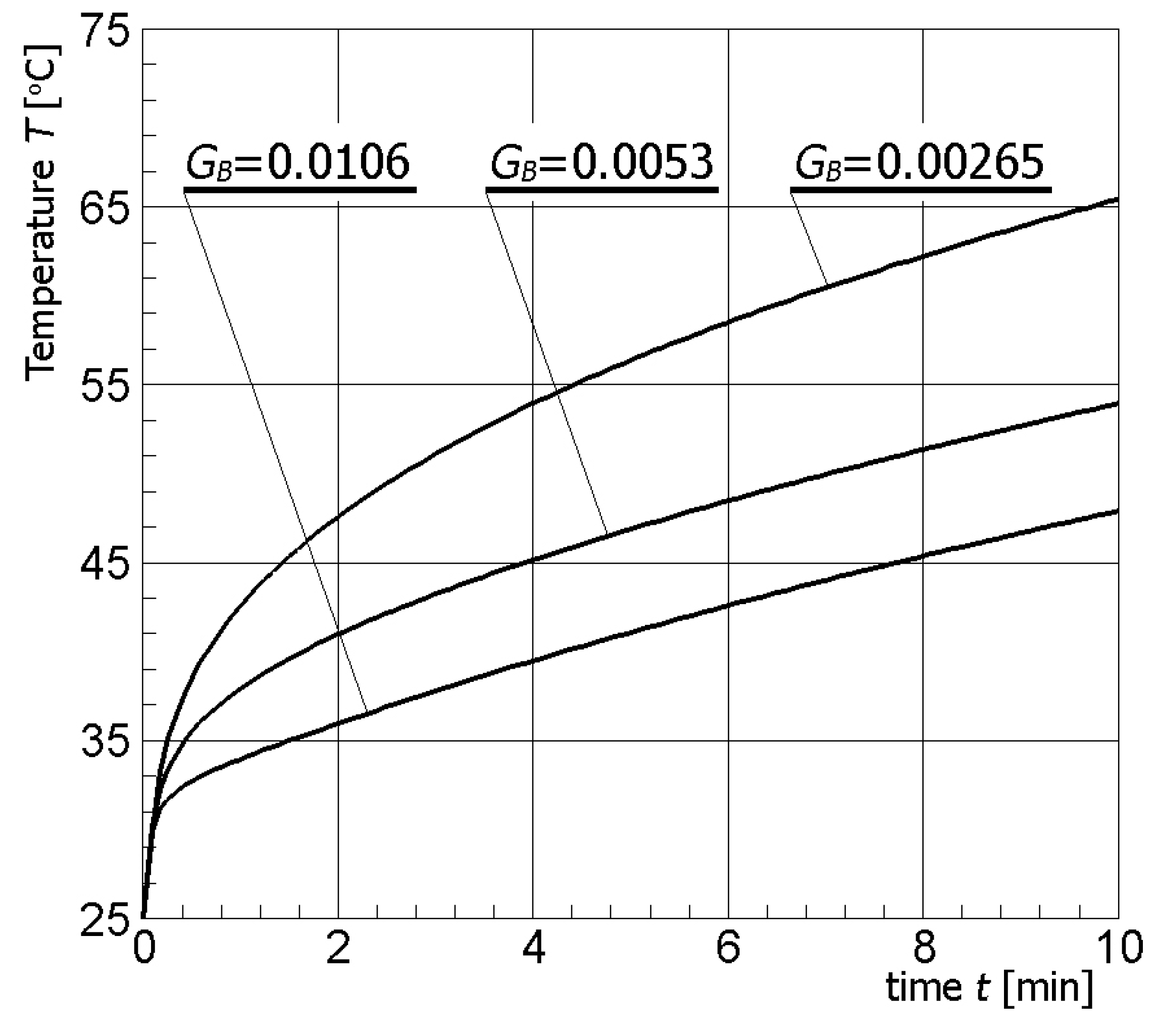
| Tumor | 0.79 | 3770 | 0.48 | 1050 | 7792 | 0.0053 |
| Blood Electrode Trocar | - 108 10−5 | 3617 840 1045 | - 18 0.026 | 1050 6450 70 | - - - | - - - |
| Tissue Type | A (1/s) | ΔE (J/mol) |
|---|---|---|
| Breast | 1.18 × 1044 | 3.02 × 10⁵ |
| Liver | 7.39 × 1039 | 2.58 × 10⁵ |
| Skin | 1.80 × 1051 | 3.27 × 10⁵ |
| Tissue with the capillaries | 1.98 × 10106 | 6.67 × 10⁵ |
| Aorta | 5.60 × 1063 | 4.30 × 10⁵ |
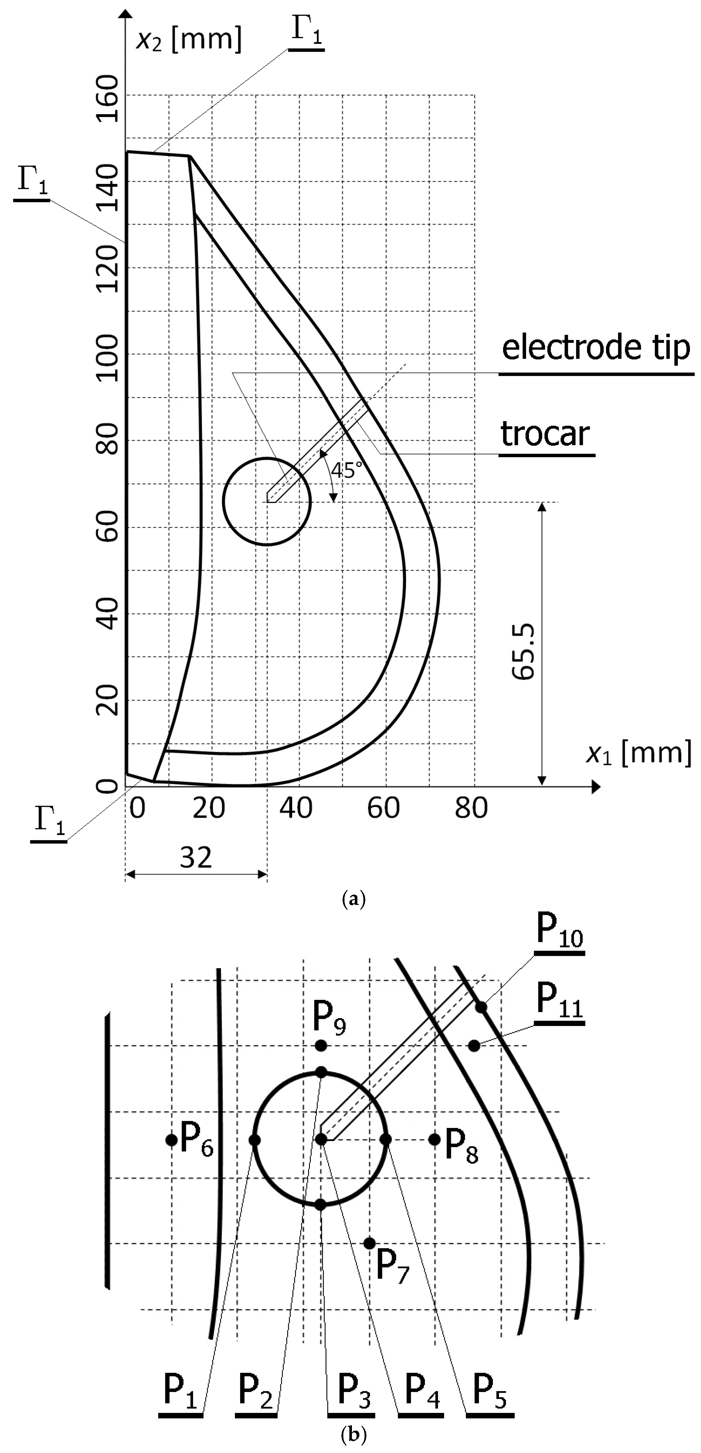
| Control Point | x (m) | y (m) |
|---|---|---|
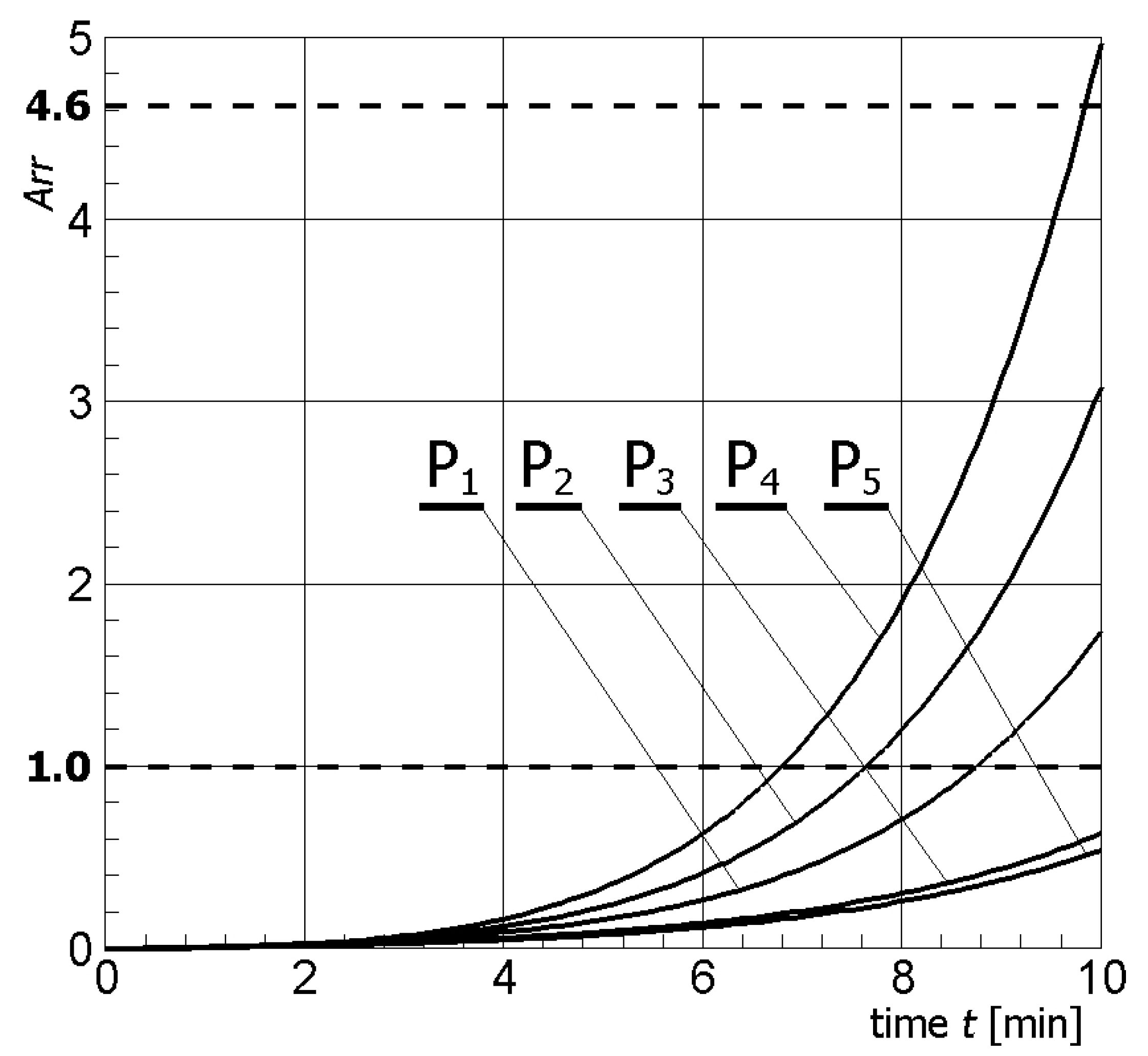
| P1 (in tumor) | 0.022 | 0.0655 |
| P2 (in tumor) | 0.032 | 0.0755 |
| P3 (in tumor) | 0.032 | 0.0555 |
| P4 (in tumor) | 0.032 | 0.0655 |
| P5 (in tumor) | 0.042 | 0.0655 |
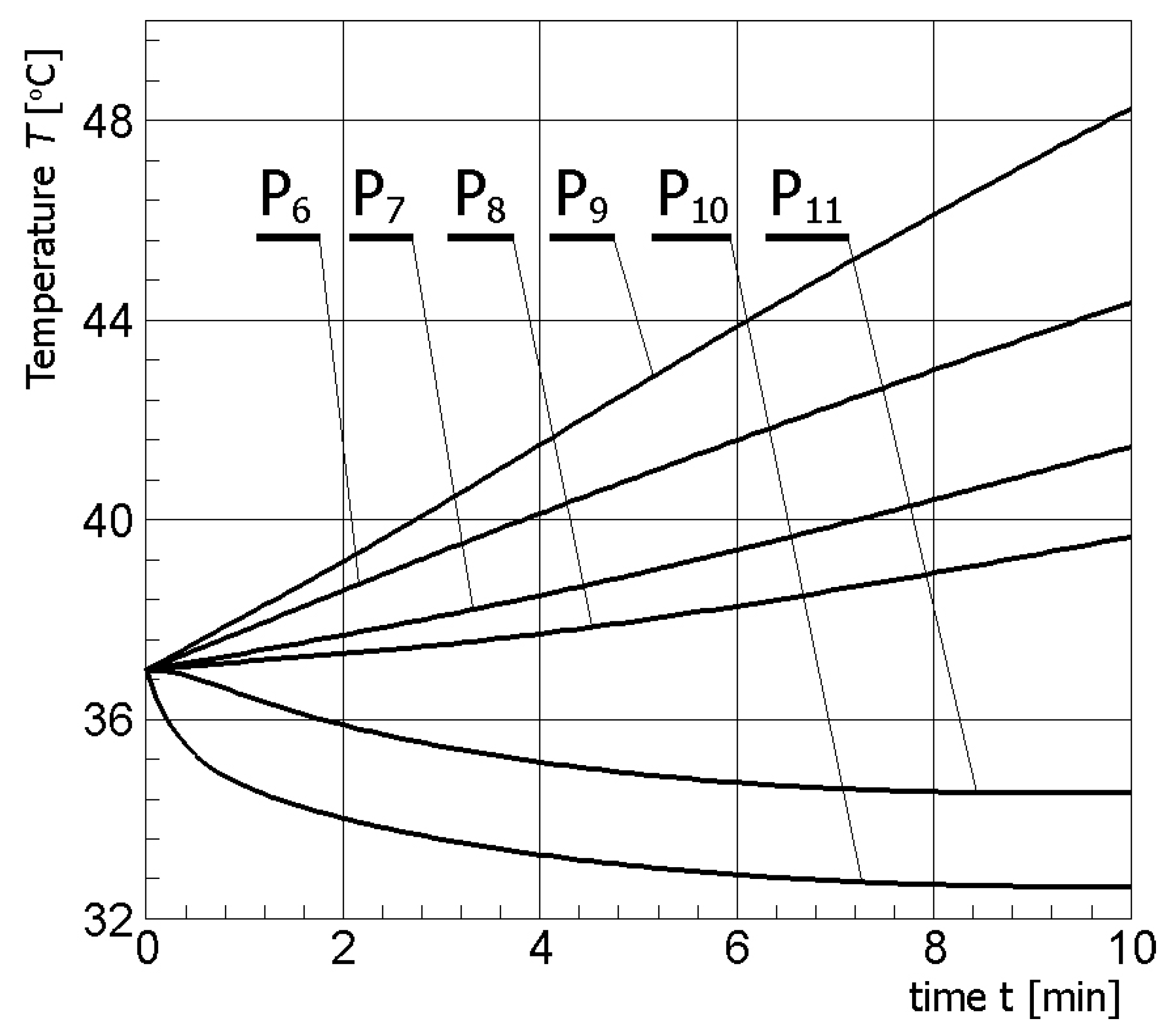
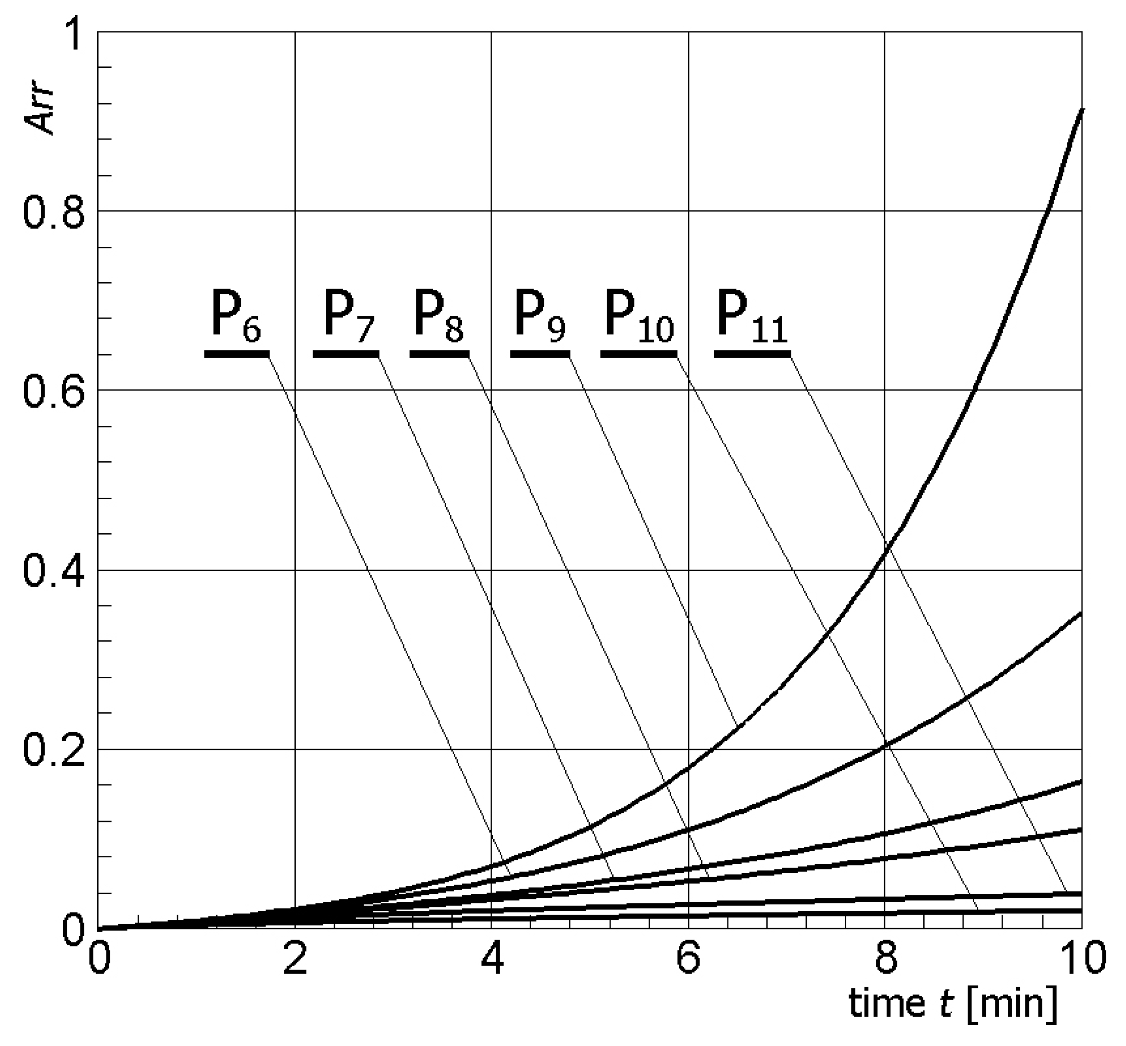
| P6 (in muscle) | 0.01 | 0.0655 |
| P7 (in gland) | 0.04 | 0.05 |
| P8 (in gland) | 0.05 | 0.0655 |
| P9 (in gland) | 0.032 | 0.08 |
| P10 (on the skin) | 0.0575 | 0.086 |
| P11 (in fat) | 0.0565 | 0.08 |
| Parameter | Value |
|---|---|
| Baseline physiological temperature TB Body core temperature Tb | 37 °C 37 °C |
| Initial temperature of the breast and tumor T1–4 Initial temperature of the electrode and trocar T5–6 | 37 °C 25 °C |
| Ambient temperature Tamb | 25 °C |
| Effective heat transfer coefficient αeff | 13.5 W/(m2K) |
| Time step Δt Length of the active part of the applicator Width of the applicator | 1 s 10 mm 1.41 mm |
| Control Point | Arr | T °C | Probability of Destruction % |
|---|---|---|---|
| P1 | 1.7388 | 50.6 | 82.43 |
| P2 | 3.0849 | 52.5 | 95.43 |
| P3 | 0.6313 | 46.9 | 46.81 |
| P4 | 4.9728 | 53.9 | 99.31 |
| P5 | 0.5393 | 46.4 | 41.68 |
| P6 | 0.3533 | 44.4 | 29.76 |
| P7 | 0.1642 | 41.5 | 15.14 |
| P8 | 0.1109 | 39.7 | 10.5 |
| P9 | 0.9155 | 48.3 | 59.97 |
| P10 | 0.021 | 32.7 | 2.08 |
| P11 | 0.0394 | 34.6 | 3.86 |
© 2019 by the author. Licensee MDPI, Basel, Switzerland. This article is an open access article distributed under the terms and conditions of the Creative Commons Attribution (CC BY) license (http://creativecommons.org/licenses/by/4.0/).
Share and Cite
Paruch, M. Mathematical Modeling of Breast Tumor Destruction Using Fast Heating during Radiofrequency Ablation. Materials 2020, 13, 136. https://doi.org/10.3390/ma13010136
Paruch M. Mathematical Modeling of Breast Tumor Destruction Using Fast Heating during Radiofrequency Ablation. Materials. 2020; 13(1):136. https://doi.org/10.3390/ma13010136
Chicago/Turabian StyleParuch, Marek. 2020. "Mathematical Modeling of Breast Tumor Destruction Using Fast Heating during Radiofrequency Ablation" Materials 13, no. 1: 136. https://doi.org/10.3390/ma13010136
APA StyleParuch, M. (2020). Mathematical Modeling of Breast Tumor Destruction Using Fast Heating during Radiofrequency Ablation. Materials, 13(1), 136. https://doi.org/10.3390/ma13010136