Finite Element Method-Based Skid Resistance Simulation Using In-Situ 3D Pavement Surface Texture and Friction Data


Abstract

1. Introduction
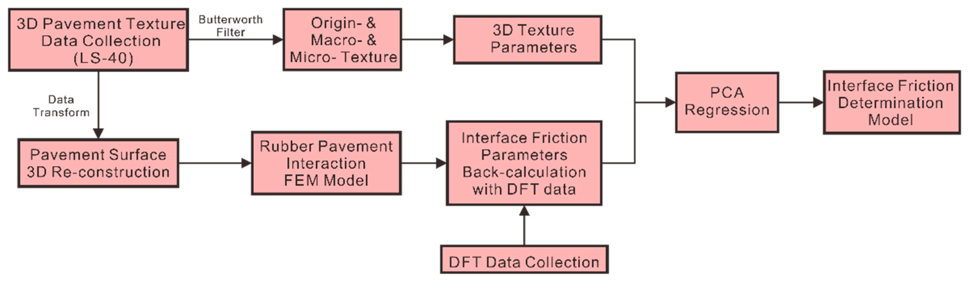
2. Objective
- Collecting in-situ high-resolution 3D pavement surface texture and skid resistance measured by the dynamic friction tester (DFT);
- Characterizing pavement texture attributes at both macro- and micro-scale with 3D areal texture parameters; the Butterworth filter is applied to separate the texture data into two scales;
- Proposing a re-construction method to establish 3D areal pavement surfaces as inputs for the FEM numerical simulation below;
- Implementing the FEM-based rubber pavement interaction model to simulate the DFT measurements;
- Computing the rubber pavement interface friction using the DFT data sets according to the binary search back-calculation method;
- Determining the relationships between rubber pavement interface friction and the 3D areal pavement texture parameters using principal component analysis PCA regression.
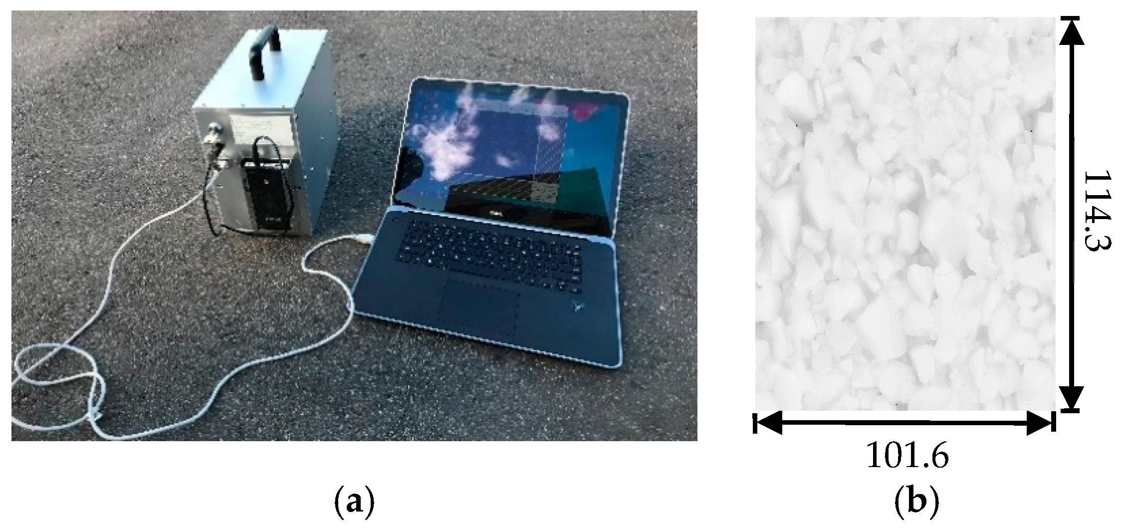
3. Field Data Collection
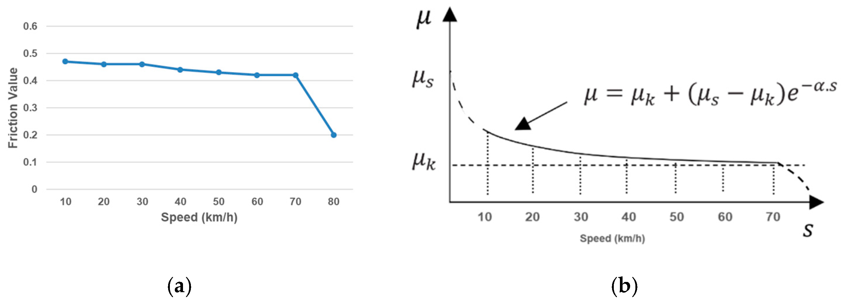
4. Interface Friction Model
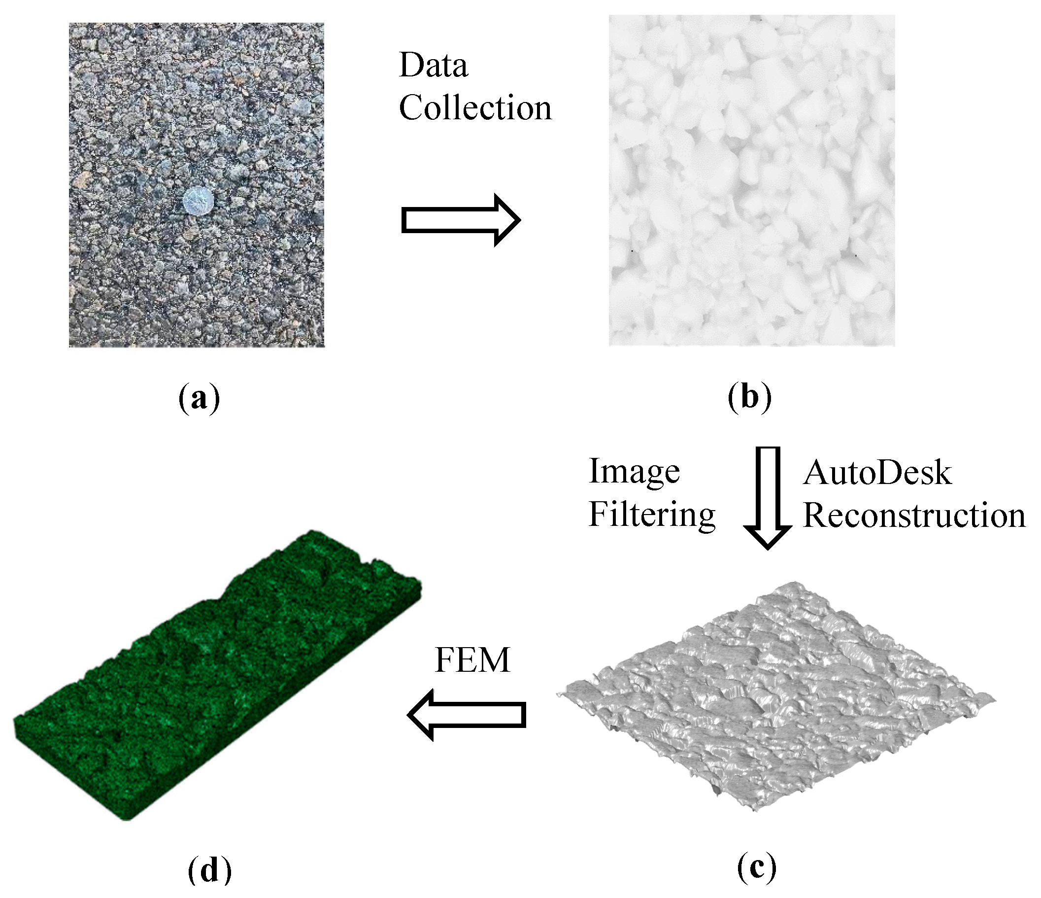
5. Reconstruction of 3D Pavement Texture Surface
6. Back-Calculation of Interface Friction Parameters
6.1. FEM Based Skid Resistance Simulation
6.2. Binary Search Back-calculation Approach
- (1)
- Calculate the midpoint value σ0 from the initial range interval [0, 0.85];
- (2)
- Input σ0 into the FEM simulation process and obtain the simulated skid number ;
- (3)
- Compare the . with the in-situ skid number . If the percentage error is less than 10%, the convergence is satisfied and the iteration process stops. Otherwise the iteration process continues and proceeds to step 4;
- (4)
- Calculate the new midpoint σ1 from the subinterval [0, σ0]. If the difference from step 3 is positive or [σ0, 0.85] if the difference is negative, feed it into the FEM simulation process for simulated skid resistance , and check whether the differences are within desired accuracy range. Repeat the process until the percentage error is less than 10%.
6.3. Validation of FEM Simulation Results
7. Friction Prediction Models Based on Surface Texture Parameters
7.1. Model Development
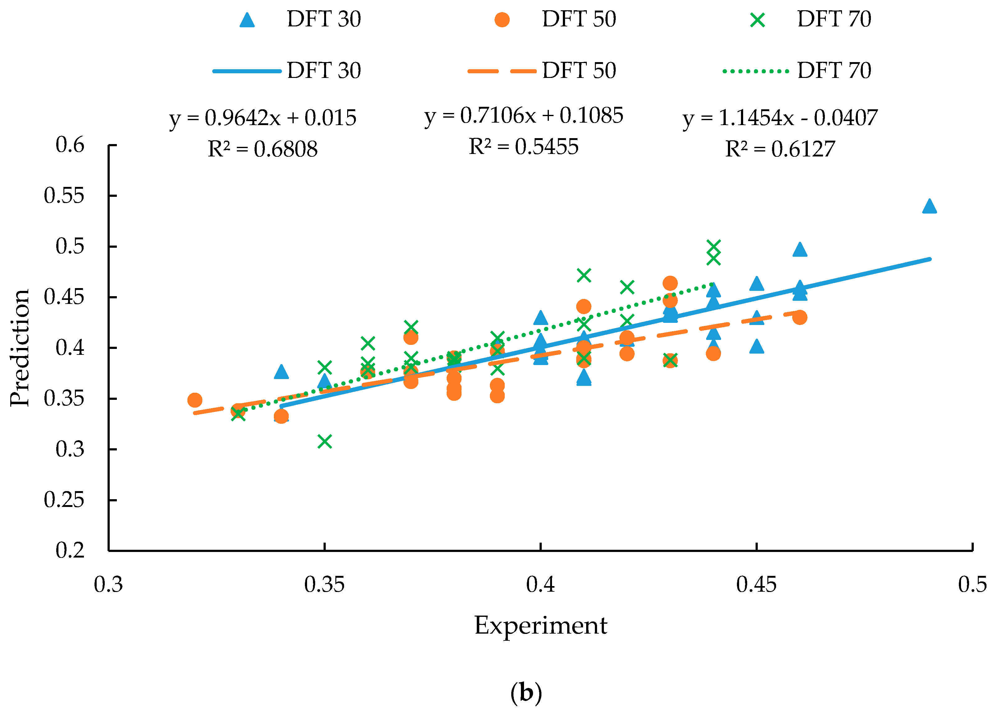
7.2. Model Verification and Discussion
8. Conclusions
- A rubber areal pavement interaction FEM model is established to determine the rubber pavement interface friction by re-constructing 3D areal pavement model from high resolution surface texture data;
- The binary search back-calculation method is used to derive the rubber pavement interface friction parameters so that the simulated skid resistance fits with the in-situ skid resistance data at a desired accuracy level;
- PCA regression models are developed to correlate interface friction parameters and the 3D areal pavement texture characteristics, which can be used to prepare the inputs of friction parameters for FEM simulation.
Author Contributions
Funding
Acknowledgments
Conflicts of Interest
References
- Fwa, T.F. Skid resistance determination for pavement management and wet-weather road safety. Int. J. Transp. Sci. Technol. 2017, 6, 217–227. [Google Scholar] [CrossRef]
- Hall, J.W.; Smith, K.L.; Titus-Glover, L. Guide for Pavement Friction Contractor’s Final Report for National Cooperative Highway Research Program (NCHRP) Project 01-43; Transportation Research Board of the National Academies: Washington, DC, USA, 2009. [Google Scholar]
- Henry, J.J. Evaluation of Pavement Friction Characteristics; Transportation Research Board: Washington, DC, USA, 2000. [Google Scholar]
- Sengoz, B.; Onsori, A.; Topal, A. Effect of aggregate shape on the surface properties of flexible pavement. KSCE J. Civ. Eng. 2014, 18, 1364–1371. [Google Scholar] [CrossRef]
- Chen, B.; Zhang, X.; Yu, J.; Wang, Y. Impact of contact stress distribution on skid resistance of asphalt pavements. Constr. Build. Mater. 2017, 133, 330–339. [Google Scholar] [CrossRef]
- Khaleghian, S.; Emami, A.; Taheri, S. A technical survey on tire-road friction estimation. Friction 2017, 5, 123–146. [Google Scholar] [CrossRef]
- Sandburg, U. Influence of Road Surface Texture on Traffic Characteristics Related to Environment, Economy, and Safety: A State-of-the-Art Study Regarding Measures and Measuring Methods; VTI Report 53A-1997; Swedish National Road Administration: Borlange, Sweden, 1998.
- Das, A.; Rosauer, V.; Bald, J.S. Study of road surface characteristics in frequency domain using micro-optical 3-D camera. KSCE J. Civ. Eng. 2015, 19, 1282–1291. [Google Scholar] [CrossRef]
- Li, T. Influencing Parameters on Tire–Pavement Interaction Noise: Review, Experiments, and Design Considerations. Designs 2018, 2, 38. [Google Scholar] [CrossRef]
- Ueckermann, A.; Wang, D.; Oeser, M.; Steinauer, B. A contribution to non-contact skid resistance measurement. Int. J. Pavement Eng. 2015, 16, 646–659. [Google Scholar] [CrossRef]
- Zelelew, H.M.; Khasawneh, M.; Abbas, A. Wavelet-based characterization of asphalt pavement surface macro-texture. Road Mater. Pavement Des. 2014, 5, 622–641. [Google Scholar] [CrossRef]
- Villani, M.M.; Scarpas, A.; de Bondt, A.; Khedoe, R.; Artamendi, I. Application of fractal analysis for measuring the effects of rubber polishing on the friction of asphalt concrete mixtures. Wear 2014, 320, 179–188. [Google Scholar] [CrossRef]
- Hartikainen, L.; Petry, F.; Westermann, S. Frequency-wise correlation of the power spectral density of asphalt surface roughness and tire wet friction. Wear 2014, 317, 111–119. [Google Scholar] [CrossRef]
- Kane, M.; Rado, Z.L.; Timmons, A. Exploring the texture-friction relationship: From texture empirical decomposition to pavement friction. Int. J. Pavement Eng. 2015, 16, 919–928. [Google Scholar] [CrossRef]
- Ueckermann, A.; Wang, D.; Oeser, M.; Steinauer, B. Calculation of skid resistance from texture measurements. J. Traffic Transp. Eng. 2015, 2, 3–16. (In English) [Google Scholar] [CrossRef]
- Li, Q.J.; Yang, G.; Wang, K.C.P.; Zhan, Y.; Wang, C. Novel macro- and micro-texture indicators for pavement friction by using high-resolution three-dimensional surface data. Transp. Res. Rec. 2017, 2641, 164–176. [Google Scholar] [CrossRef]
- Tanner, J.A. Computational Methods for Frictional Contact with Applications to the Space Shuttle Orbiter Nose-Gear Tire; NASA Technical Paper No. 3574; NASA, Langley Research Center: Hampton, VA, USA, 1996.
- Davis, P.A. Quasi-Static and Dynamic Response Characteristics of f-4 Bias-Ply and Radial-Belted Main Gear Tires; NASA Technical Paper 3586; NASA, Langley Research Center: Hampton, VA, USA, 1997.
- Johnson, A.R.; Tanner, J.A.; Mason, A.J. Quasi-Static Viscoelastic Finite Element Model of an Aircraft Tire; NASA/TM-1999-209141; NASA, Langley Research Center: Hampton, VA, USA, 1999.
- Cho, J.R.; Lee, H.W.; Sohn, J.S.; Kim, G.J.; Woo, J.S. Numerical investigation of hydroplaning characteristics of three-dimensional patterned tire. Eur. J. Mech. Solids 2006, 25, 914–926. [Google Scholar] [CrossRef]
- Wollny, I.; Behnke, R.; Villaret, K.; Kaliske, M. Numerical modeling of tyre–pavement interaction phenomena: Coupled structural investigations. Road Mater. Pavement Des. 2016, 17, 563–578. [Google Scholar] [CrossRef]
- Acosta, M.; Kanarachos, S.; Blundell, M. Road Friction Virtual Sensing: A Review of Estimation Techniques with Emphasis on Low Excitation Approaches. Appl. Sci. 2017, 7, 1230. [Google Scholar] [CrossRef]
- Savkoor, A.R. Mechanics of sliding friction of elastomers. Wear 1986, 113, 37–60. [Google Scholar] [CrossRef]
- Ma, B.; Xu, H.-G.; Liu, H.-F. Effects of road surface fractal and rubber characteristics on tire sliding friction factor. J. Jilin Univ. Eng. Technol. Ed. 2013, 43, 317–322. [Google Scholar]
- Li, Z.; Li, Z.R.; Xia, Y.M. Experimental and numerical study of frictional contact behavior of rolling tire. J. Shanghai Jiaotong Univ. 2013, 47, 817–821. [Google Scholar]
- Dorsch, V.; Becker, A.; Vossen, L. Enhanced rubber friction model for finite element simulations of rolling tyres. Plast. Rubber Compos. 2002, 31, 458–464. [Google Scholar] [CrossRef]
- Tielking, J.T.; Roberts, F.L. Tire contact pressure and its effect on pavement strain. J. Transp. Eng. 1987, 113, 56–71. [Google Scholar] [CrossRef]
- Roque, R.; Myers, L.; Birgisson, B. Evaluating measured tire contact stresses to predict pavement response and performance. Transp. Res. Rec. 2000, 1716, 73–81. [Google Scholar] [CrossRef]
- Ghoreishy, M.H.R.; Malekzadeh, M.; Rahimi, H. A parametric study on the steady state rolling behaviour of a steel-belted radial tyre. Iran. Polym. J. 2007, 16, 539–548. [Google Scholar]
- Wang, H.; Al-Qadi, I. Combined effect of moving wheel loading and three-dimensional contact stresses on perpetual pavement responses. Transp. Res. Rec. 2009, 2095, 53–61. [Google Scholar] [CrossRef]
- Fwa, T.F.; Ong, G.P. Wet-pavement hydroplaning risk and skid resistance: Analysis. J. Transp. Eng. 2008, 134, 182–190. [Google Scholar] [CrossRef]
- Wang, H.; Al-Qadi, I.L.; Stanciulescu, I. Effect of surface friction on tire-pavement contact stresses during vehicle maneuvering. J. Eng. Mech. 2014, 140, 0401400. [Google Scholar] [CrossRef]
- Zhou, H.; Wang, G.; Ding, Y.; Yang, J.; Liang, C.; Fu, J. Effect of friction model and tire maneuvering on tire-pavement contact stress. Adv. Mater. Sci. Eng. 2015, 2015, 632647. [Google Scholar] [CrossRef]
- Oden, J.T.; Martins, J.A.C. Models and computational methods for dynamic friction phenomena. Comput. Methods Appl. Mech. Eng. 1985, 52, 527–634. [Google Scholar] [CrossRef]
- Anupam, K.; Srirangam, S.K.; Scarpas, A.; Kasbergen, C. Influence of Temperature on Tire–Pavement Friction: Analyses. Transp. Res. Rec. 2013, 2369, 114–124. [Google Scholar] [CrossRef]
- Srirangam, S.K.; Anupam, K.; Scarpas, A.; Kösters, A. Influence of Temperature on Tire-Pavement Friction-1: Laboratory Tests and Finite Element Modeling. In Proceedings of the 92nd Annual Meeting of the Transportation Research Board, Washington, DC, USA, 13–17 January 2013. [Google Scholar]
- Srirangam, S.K.; Anupam, K.; Kasbergen, C.; Scarpas, A. Study of Influence of Operating Parameters on Braking Friction and Rolling Resistance. Transp. Res. Rec. 2015, 2525, 79–90. [Google Scholar] [CrossRef]
- Tang, T.; Anupam, K.; Kasbergen, C.; Kogbara, R.; Scarpas, A.; Masad, E. Finite Element Studies of Skid Resistance under Hot Weather Condition. Transp. Res. Rec. 2018, 2672. [Google Scholar] [CrossRef]
- Puccinelli, J. Long-Term Pavement Performance Warm Mix Asphalt Study; Daft Final Report, Contract No. DTFH61-12-C-00017; Federal Highway Administration: Mclean, VA, USA, 2014.
- Li, S.; Noureldin, S.; Zhu, K.; Jiang, Y. Pavement Surface Microtexture: Testing, Characterization and Frictional Interpretation; STP1555; ASTM International: Conshohocken, PA, USA, 2012. [Google Scholar]
- ASTM Standard E1911-09a. Standard Test Method for Measuring Paved Surface Frictional Properties Using the Dynamic Friction Tester; ASTM International: West Conshohocken, PA, USA, 2009.
- Mataei, B.; Zakeri, H.; Zahedi, M.; Nejad, F.M. Pavement friction and skid resistance measurement methods: A literature review. Open J. Civ. Eng. 2016, 6, 537–565. [Google Scholar] [CrossRef]
- Tamboli, K.; Athre, K. Experimental investigations on water lubricated hydrodynamic bearing. Procedia Technol. 2016, 23, 68–75. [Google Scholar] [CrossRef]
- Schwarzer, N. Modelling of Contact Problems of Rough Surfaces; Publication of the Saxonian Institute of Surface Mechanics: Eilenburg, Germany, 2007. [Google Scholar]
- Zhang, L.; Fwa, T.F.; Ong, G.P.; Chu, L. Analysing effect of roadway width on skid resistance of porous pavement. Road Mater. Pavement Des. 2013, 17, 1–14. [Google Scholar] [CrossRef]
- Kosgolla, J.V. Numerical Simulation of Sliding Friction and Wet Traction Force on a Smooth Tire Sliding on a Random Rough Pavement. Ph.D. Thesis, University of South Florida, Tampa, FL, USA, 2012. [Google Scholar]
- Tao, Q.; Lee, H.P.; Lim, S.P. Contact mechanics of surfaces with various models of roughness descriptions. Wear 2001, 249, 539–545. [Google Scholar] [CrossRef]
- Hyun, S.; Pei, L.; Molinari, J.F.; Robbins, M.O. Finite-element analysis of contact between elastic self-affine surfaces. Phy. Rev. E 2004, 70, 026117. [Google Scholar] [CrossRef]
- Thompson, M.K.; Thompson, J.M. Considerations for the incorporation of measured surfaces in finite element models. Scanning 2010, 32, 183–198. [Google Scholar] [CrossRef]
- Pawar, G.; Pawlus, P.; Etsion, I.; Raeymaekers, B. The effect of determining topography parameters on analyzing elastic contact between isotropic rough surfaces. J. Tribol. 2013, 135, 1–10. [Google Scholar] [CrossRef]
- Peter, K. Beanplot: A Boxplot Alternative for Visual Comparison of Distributions. J. Stat. Softw. 2008, 28, 1–9. [Google Scholar]
- AutoCAD 2013 User’s Guide; Autodesk, Inc.: San Rafae, CA, USA, 2013.
- Zuniga-Garcia, N.; Prozzi, J.A. Contribution of Micro-and Macro-Texture for Predicting Friction on Pavement Surfaces; CHPP Report-UTA# 3-2016; University Transportation Center for Highway Pavement Preservation, Michigan State University: East Lansing, MI, USA, 2016. [Google Scholar]
- ABAQUS User’s Manual; Version 6.13; Dassault Systèmes: Paris, France, 2013.
- Srirangam, S.K. Numerical Simulation of Tire-Pavement Interaction. PhD Thesis, Delft University of Technology, Delft, The Netherlands, 2015. [Google Scholar]
- Wilson, D.J.; Dunn, R. Analyzing Road Pavement Skid Resistance. In ITE 2005 Annual Meeting and Exhibit Compendium of Technical Papers; Institute of Transportation Engineers (ITE) ARRB Group Ltd.: Washington, DC, USA, 2005. [Google Scholar]
- ASTM E501-94. Standard Specification for Standard Rib Tire for Pavement Skid-Resistance Tests; ASTM International: West Conshohocken, PA, USA, 2000.
- ASTM E1844-08. Standard Specification for A Size 10 × 4–5 Smooth-Tread Friction Test Tire; ASTM International: West Conshohocken, PA, USA, 2015.
- ASTM E524-88. Standard Specification for Standard Smooth Tire for Pavement Skid-Resistance Tests; ASTM International: West Conshohocken, PA, USA, 2000.
- Ong, G.P.; Fwa, T.F. Wet-pavement hydroplaning risk and skid resistance: Modeling. J. Transp. Eng. 2008, 133, 590–598. [Google Scholar] [CrossRef]
- Zegard, A.; Helmand, F.; Tang, T.; Anupam, K.; Scarpas, A. Rheological Properties of Tire Rubber using Dynamic Shear Rheometer for FEM Tire-Pavement Interaction Studies. In Proceedings of the Eighth International Conference on Maintenance and Rehabilitation of Pavements, Singapore, 27–29 July 2016. [Google Scholar]
- Srirangam, S.K.; Anupam, K.; Kasbergen, C.; Scarpas, A. Analysis of asphalt mix surface-tread rubber interaction by using finite element method. J. Traffic Transp. Eng. 2017, 4, 395–402. (In English) [Google Scholar] [CrossRef]
- Michelin. The Tyre, Grip; Société de Technologie Michelin: Clermont-Ferrand, France, 2001. [Google Scholar]
- Kawa, I.; Hayhoe, G.F. Development of a Computer Program to Compute Pavement Thickness and Strength. In Proceedings of the 2002 Federal Aviation Administration Airport Technology Transfer Conference, Atlantic, NJ, USA, May 2002; Atlantic City International Airport: Egg Harbor, NJ, USA, 2002. [Google Scholar]
- Jolliffe, I.T. Principal Component Analysis, 2nd ed.; Springer: New York, NY, USA, 2002. [Google Scholar]
- Abdi, H.; Williams, L.J. Principal component analysis. Interdiscip. Rev. Comput. Stat. 2010, 2, 433–459. [Google Scholar] [CrossRef]
- Leach, R. (Ed.) Characterisation of Areal Surface Texture; Springer Science & Business Media: Berlin/Heidelberg, Germany, 2013. [Google Scholar]
- ISO. Geometrical Product Specifications (GPS)—Surface Texture: Areal—Part 2: Terms, Definitions and Surface Texture Parameters; ISO 25178-2:2012(en); ISO: London, UK, 2012. [Google Scholar]
- Oufqir, S.; Bloom, P.R.; Toner, B.M.; El Azzouzi, M. Surface characterization of natural and Ca-saturated soil humic-clay composites at the micrometer scale: Effect of Calcium. J. Mater. Environ. Sci. 2015, 6, 3174–3183. [Google Scholar]
- Klauer, K.; Eifler, M.; Seewig, J.; Kirsch, B.; Aurich, J.C. Application of function-oriented roughness parameters using confocal microscopy. Eng. Sci. Technol. Int. J. 2018, 21, 302–313. [Google Scholar] [CrossRef]
- Löberg, J.; Mattisson, I.; Hansson, S.; Ahlberg, E. Characterisation of titanium dental implants I: Critical assessment of surface roughness parameters. Open Biomater. J. 2010, 2, 18–35. [Google Scholar] [CrossRef]


| Section ID | Binder | Comment | Aggregate Combination |
|---|---|---|---|
| E1 | PG 70-28 | HMA with RAP + RAS | 1 |
| E2 | PG 70-28 | WMA foaming with RAP + RAS | 1 |
| E3 | PG 70-28 | WMA chemical with RAP + RAS | 1 |
| E4 | PG 64-22 | WMA chemical with RAP + RAS | 1 |
| E5 | PG 58-28 | WMA chemical with RAP + RAS | 1 |
| E6 | PG 70-28 | WMA stone mix with mineral filler | 2 |
| C1–C6 | PG 70-28 | HMA with RAP | 3 |
| No. | μs | μk | α | No. | μs | μk | α |
|---|---|---|---|---|---|---|---|
| 1 | 0.4 | 0.35 | 0.5 | 15 | 0.4 | 0.36 | 0.2 |
| 2 | 0.4 | 0.35 | 0.5 | 16 | 0.4 | 0.36 | 0.2 |
| 3 | 0.4 | 0.36 | 0.2 | 17 | 0.4 | 0.36 | 0.2 |
| 4 | 0.4 | 0.39 | 0.6s | 18 | 0.4 | 0.35 | 0.6 |
| 5 | 0.5 | 0.31 | 0.6 | 19 | 0.4 | 0.39 | 0.6 |
| 6 | 0.5 | 0.23 | 0.4 | 20 | 0.5 | 0.35 | 0.6 |
| 7 | 0.5 | 0.35 | 0.6 | 21 | 0.5 | 0.4 | 0.2 |
| 8 | 0.4 | 0.35 | 0.6 | 22 | 0.5 | 0.36 | 0.2 |
| 9 | 0.4 | 0.33 | 0.6 | 23 | 0.5 | 0.34 | 0.2 |
| 10 | 0.4 | 0.34 | 0.6 | 24 | 0.4 | 0.37 | 0.6 |
| 11 | 0.4 | 0.34 | 0.6 | 25 | 0.5 | 0.4 | 0.2 |
| 12 | 0.4 | 0.35 | 0.6 | 26 | 0.5 | 0.3 | 0.2 |
| 13 | 0.4 | 0.35 | 0.6 | 27 | 0.4 | 0.37 | 0.6 |
| 14 | 0.4 | 0.35 | 0.6 | ||||
| Texture Parameter | Category | Definition | Unit |
|---|---|---|---|
| Sq | Height parameters | Root-mean-square height | mm |
| Ssk | Skewness | ||
| Sp | Maximum peak height | mm | |
| Sv | Maximum pit height | mm | |
| Sz | Maximum height | mm | |
| Sa | Arithmetic mean height | mm | |
| Fdmax | Maximum depth of surface furrows in the height parameters | mm | |
| Fdmean | Mean depth of surface furrows in the height parameters | mm | |
| Fden | Mean density of surface furrows in the height parameters | cm/cm2 | |
| Sal | Spatial parameters | Autocorrelation length | mm |
| Str | Texture-aspect ratio | ||
| Sdq | Hybrid parameters | Root-mean-square gradient | |
| Sdr | Developed interfacial area ratio | % | |
| Vm | Volume parameters | Material volume | mm3/mm2 |
| Vv | Void volume | mm3/mm2 | |
| Vmp | Peak material volume | mm3/mm2 | |
| Vmc | Core material volume | mm3/mm2 | |
| Vvc | Core void volume | mm3/mm2 | |
| Vvv | Pit void volume | mm3/mm2 | |
| Sk | Core roughness depth | mm | |
| Spk | Reduced summit height | mm | |
| Svk | Reduced valley depth | mm | |
| Spc | Arithmetic mean peak curvature | 1/mm | |
| S10z | Ten point height | mm | |
| S5p | Five point peak height | mm | |
| S5v | Five point pit height | mm | |
| Shv | Mean hill volume | mm3 | |
| Sa2 | Functional parameters | Areas below the material ratio curve | mm3/mm2 |
| Sr1 | Upper bearing area | % | |
| Sr2 | Lower bearing area | % | |
| Threshold | Islands parameters | The threshold value to estimate the bumps contained in the height parameters | mm |
| Mean Volume | Mean volume of the islands | mm3 | |
| Mean Height/Surface ratio | Mean ratio of the height to surface of the islands | mm/mm2 | |
| Mean Area | Motifs parameters | Mean area of the motifs | mm |
| Temperature | Pavement surface temperature | °C | |
| Statistical Results | Average | Maximum | Minimum | Standard Deviation | |||||
|---|---|---|---|---|---|---|---|---|---|
| Parameters | Macro | Micro | Macro | Micro | Macro | Micro | Macro | Micro | |
| Sq | 0.37 | 0.02 | 0.87 | 0.04 | 0.22 | 0.02 | 0.17 | 0.01 | |
| Ssk | −1.66 | −0.33 | 0.02 | 0.02 | −2.54 | −0.64 | 0.55 | 0.13 | |
| Sp | 1.77 | 0.42 | 4.93 | 0.84 | 0.89 | 0.21 | 0.95 | 0.16 | |
| Sv | 2.81 | 0.51 | 3.72 | 0.96 | 1.88 | 0.24 | 0.49 | 0.18 | |
| Sz | 4.59 | 0.93 | 8.57 | 1.69 | 3.22 | 0.47 | 1.21 | 0.32 | |
| Sa | 0.26 | 0.02 | 0.67 | 0.02 | 0.15 | 0.01 | 0.14 | 0.002 | |
| Fdmax | 3.05 | 0.35 | 4.61 | 0.62 | 2.01 | 0.20 | 0.62 | 0.12 | |
| Fden | 11.64 | 18.80 | 12.93 | 19.03 | 8.66 | 18.61 | 1.20 | 0.11 | |
| Sal | 2.90 | 0.19 | 4.49 | 0.19 | 2.04 | 0.18 | 0.49 | 0.001 | |
| Str | 0.72 | 0.20 | 0.93 | 0.29 | 0.51 | 0.005 | 0.10 | 0.08 | |
| Sdq | 0.63 | 0.23 | 1.27 | 0.47 | 0.44 | 0.17 | 0.20 | 0.07 | |
| Sdr | 15.41 | 2.52 | 40.89 | 7.11 | 8.28 | 1.41 | 7.84 | 1.31 | |
| Vm | 0.01 | 0.002 | 0.03 | 0.003 | 0.01 | 0.002 | 0.006 | 0.002 | |
| Vv | 0.37 | 0.03 | 0.99 | 0.03 | 0.21 | 0.02 | 0.20 | 0.003 | |
| Vmp | 0.01 | 0.002 | 0.03 | 0.002 | 0.01 | 0.007 | 0.01 | 0.004 | |
| Vmc | 0.26 | 0.01 | 0.76 | 0.02 | 0.14 | 0.01 | 0.16 | 0.002 | |
| Vvc | 0.30 | 0.02 | 0.86 | 0.03 | 0.17 | 0.02 | 0.18 | 0.001 | |
| Vvv | 0.07 | 0.003 | 0.15 | 0.01 | 0.04 | 0.002 | 0.03 | 0.003 | |
| Sk | 0.63 | 0.04 | 1.92 | 0.05 | 0.36 | 0.04 | 0.39 | 0.003 | |
| Spk | 0.28 | 0.03 | 0.67 | 0.07 | 0.15 | 0.02 | 0.12 | 0.01 | |
| Svk | 0.70 | 0.04 | 1.45 | 0.07 | 0.39 | 0.02 | 0.26 | 0.01 | |
| Spc | 9.15 | 10.45 | 45.01 | 47.14 | 5.43 | 4.30 | 8.74 | 11.06 | |
| S10z | 3.19 | 0.68 | 6.29 | 1.38 | 2.18 | 0.41 | 0.93 | 0.22 | |
| S5p | 1.07 | 0.32 | 3.20 | 0.67 | 0.35 | 0.19 | 0.63 | 0.11 | |
| S5v | 2.12 | 0.37 | 3.09 | 0.71 | 1.40 | 0.21 | 0.42 | 0.11 | |
| Shv | 1.81 | 0.03 | 6.26 | 0.12 | 0.70 | 0.01 | 1.40 | 0.02 | |
| Sa2 | 0.0595 | 0.0022 | 0.1303 | 0.0046 | 0.0316 | 0.0012 | 0.0221 | 0.0007 | |
| Sr1 | 8.64 | 11.4427 | 11.28 | 13.999 | 7.25 | 10.429 | 1.01 | 0.7643 | |
| Sr2 | 82.54 | 88.2025 | 84.97 | 89.333 | 81.15 | 87.317 | 1.03 | 0.5326 | |
| Threshold | 1.6029 | 0.3999 | 4.4747 | 0.8204 | 0.862 | 0.2094 | 0.7711 | 0.1268 | |
| Mean Volume | 10135 | 890.9 | 22357 | 3566.1 | 0.32 | 0.0022 | 7925.8 | 1131.04 | |
| Mean Height/Surface ratio | 1.2094 | 1.0105 | 13.5843 | 13.132 | 0.0002 | 2.929 | 2.9249 | 2.5314 | |
| Mean Area | 45.906 | 6.5764 | 106.636 | 14.94 | 25.104 | 2.4568 | 18.215 | 3.3 | |
| Temperature | 15.8 | 15.8 | 18.9 | 18.9 | 11.8 | 11.8 | 3.64 | 3.64 | |
| Component | μs | μk | α | ||||
|---|---|---|---|---|---|---|---|
| Coefficient | p-Value | Coefficient | p-Value | Coefficient | p-Value | ||
| Intercept | 4.503 × 10−01 | *** | 3.504 × 10−01 | *** | 4.519 × 10−01 | *** | |
| 1 | 0.1022 × 10−01 | ** | −0.03165 × 10−01 | *** | −0.1298 × 10−01 | * | |
| 2 | 0.2557 × 10−01 | *** | 0.04643 × 10−01 | ** | −0.4774 × 10−01 | * | |
| 3 | −0.1781 × 10−01 | ** | 0.2217 × 10−01 | *** | 0.7817 × 10−01 | * | |
| 4 | 0.4148 × 10−01 | ** | 0.1323 × 10−01 | * | −5.040 × 10−01 | * | |
| 5 | 0.7041 × 10−01 | *** | 0.2229 × 10−01 | * | 41.24 × 10−01 | ** | |
| 6 | −1.349 × 10−01 | *** | −7.055 × 10−01 | *** | −63.63 × 10−01 | ** | |
| 7 | 2.895 × 10−01 | *** | 12.98 × 10−01 | ** | 228.3 × 10−01 | ** | |
| 8 | −4.715 × 10−01 | *** | −17.40 × 10−01 | * | −767.0 × 10−01 | ** | |
| 9 | −2.459 × 10−01 | ** | −22.91 × 10−01 | ** | −1786.0 × 10−01 | *** | |
| 10 | 3.975 × 10−01 | *** | |||||
| 11 | −13.93 × 10−01 | *** | |||||
| 12 | −187.3 × 10−01 | *** | |||||
| 13 | 114.0 × 10−01 | *** | |||||
| 14 | −1120.0 × 10−01 | *** | |||||
| 15 | 699.5 × 10−01 | *** | |||||
| 16 | −313.8 × 10−01 | *** | |||||
| 17 | 1933.0 × 10−01 | *** | |||||
| Validation Results | p-value | *** | *** | *** | |||
| R2 | 9.812 × 10−01 | 8.873 × 10−01 | 8.179 × 10−01 | ||||
| Adjusted R2 | 9.456 × 10−01 | 8.276 × 10−01 | 7.215 × 10−01 | ||||
| RSE | 0.1027 × 10−01 | 0.1379 × 10−01 | 0.9858 × 10−01 | ||||
| No. of Samples | 27 | ||||||
| Item | μs | μk | α | Item | μs | μk | α | ||
|---|---|---|---|---|---|---|---|---|---|
| Coefficient | Coefficient | Coefficient | Coefficient | Coefficient | Coefficient | ||||
| Macro | Micro | Micro | Macro | Macro | Micro | Micro | Macro | ||
| Intercept | 0.0029 | −0.0336 | 0.7926 | Vvc | −0.0250 | −0.9959 | 0.0187 | ||
| Sq | 1.2279 | −0.0786 | 0.0217 | Vvv | 9.2543 | −0.6802 | 0.2615 | ||
| Ssk | 0.0076 | Sk | −0.0103 | 0.0106 | |||||
| Sp | 0.0012 | Spk | 0.3215 | −0.1864 | |||||
| Sv | 0.0328 | Svk | 0.3706 | −0.0115 | 0.0275 | ||||
| Sz | 0.0011 | Spc | −0.0008 | −0.0004 | −0.0002 | ||||
| Sa | −0.7194 | 0.0345 | S10z | −0.0277 | |||||
| Fdmax | 0.0187 | S5p | 0.0099 | 0.0023 | |||||
| Fdmean | −0.0152 | −0.2727 | 0.0083 | S5v | 0.0253 | ||||
| Fden | 0.0197 | Shv | −0.0151 | ||||||
| Sal | 4.5669 | −0.67 | −6.1146 | Sa2 | 7.2769 | −0.3313 | |||
| Str | −0.0280 | Sr1 | 0.0121 | −0.0007 | |||||
| Sdq | 0.0152 | 0.0349 | 0.054 | Sr2 | 0.0025 | ||||
| Sdr | 0.0004 | 0.0023 | 0.0001 | 0.0015 | Threshold | 0.0012 | |||
| Vm | 4.3611 | −3.275 | Mean Height/Surface ratio | −0.0017 | 0.0003 | −0.0002 | |||
| Vv | −0.0182 | −0.6727 | 0.0195 | Mean Area | −0.0934 | ||||
| Vmp | 4.3611 | −3.275 | Temperature | 0.0004 | −0.0022 | ||||
| Vmc | −0.0226 | −1.7592 | 0.0317 | ||||||
© 2019 by the authors. Licensee MDPI, Basel, Switzerland. This article is an open access article distributed under the terms and conditions of the Creative Commons Attribution (CC BY) license (http://creativecommons.org/licenses/by/4.0/).
Share and Cite
Peng, Y.; Li, J.Q.; Zhan, Y.; Wang, K.C.P.; Yang, G. Finite Element Method-Based Skid Resistance Simulation Using In-Situ 3D Pavement Surface Texture and Friction Data. Materials 2019, 12, 3821. https://doi.org/10.3390/ma12233821
Peng Y, Li JQ, Zhan Y, Wang KCP, Yang G. Finite Element Method-Based Skid Resistance Simulation Using In-Situ 3D Pavement Surface Texture and Friction Data. Materials. 2019; 12(23):3821. https://doi.org/10.3390/ma12233821
Chicago/Turabian StylePeng, Yi, Joshua Qiang Li, You Zhan, Kelvin C. P. Wang, and Guangwei Yang. 2019. "Finite Element Method-Based Skid Resistance Simulation Using In-Situ 3D Pavement Surface Texture and Friction Data" Materials 12, no. 23: 3821. https://doi.org/10.3390/ma12233821
APA StylePeng, Y., Li, J. Q., Zhan, Y., Wang, K. C. P., & Yang, G. (2019). Finite Element Method-Based Skid Resistance Simulation Using In-Situ 3D Pavement Surface Texture and Friction Data. Materials, 12(23), 3821. https://doi.org/10.3390/ma12233821