The Fitting of a Fiber-Reinforced-Plastic Complex Curved Surface and Its Orbit Optimization Model with Belt Grinding Line Contact


Abstract
1. Introduction
2. Glass Radome Complex Surface Mathematical Experiment
2.1. Modeling and Error Analysis of FRP Complex Surface Based on Least-Squares Method
2.2. Trajectory Planning for Abrasive Belt Grinding
3. Materials and Methods
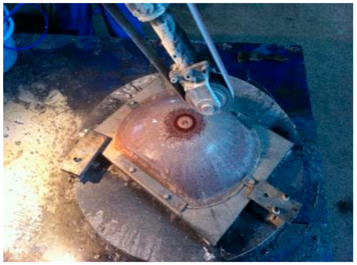
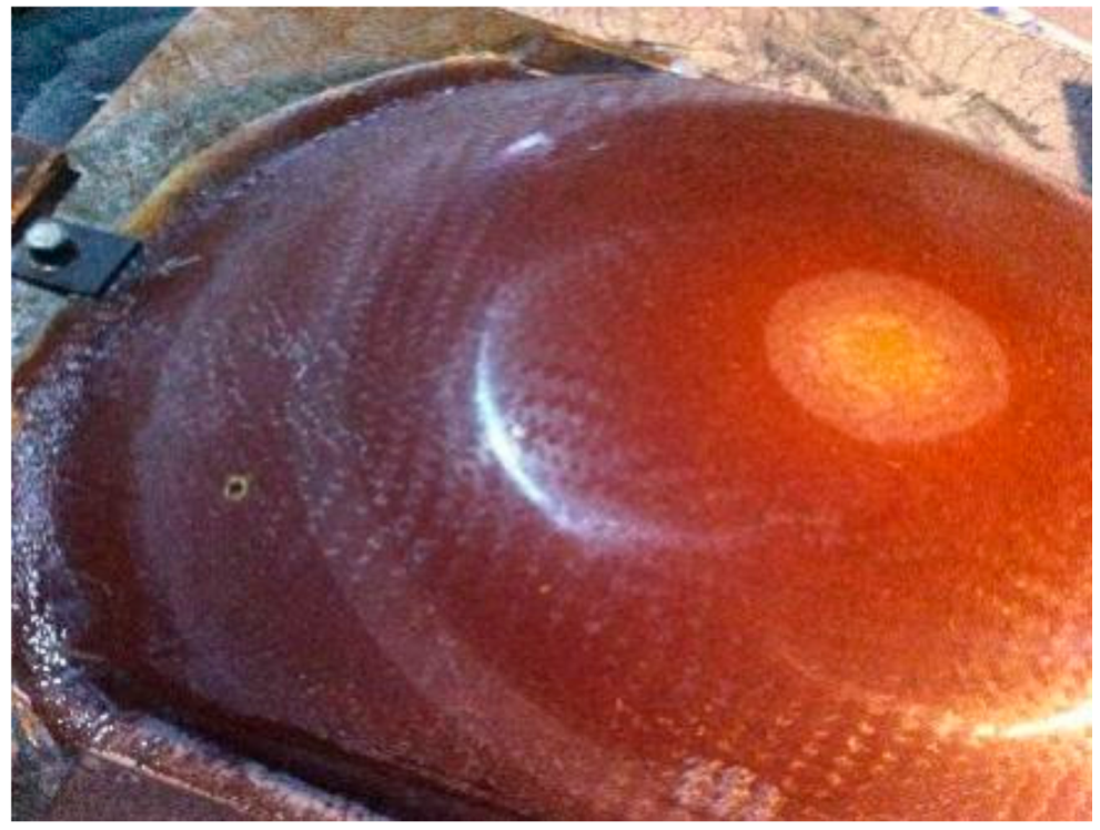
3.1. Materials
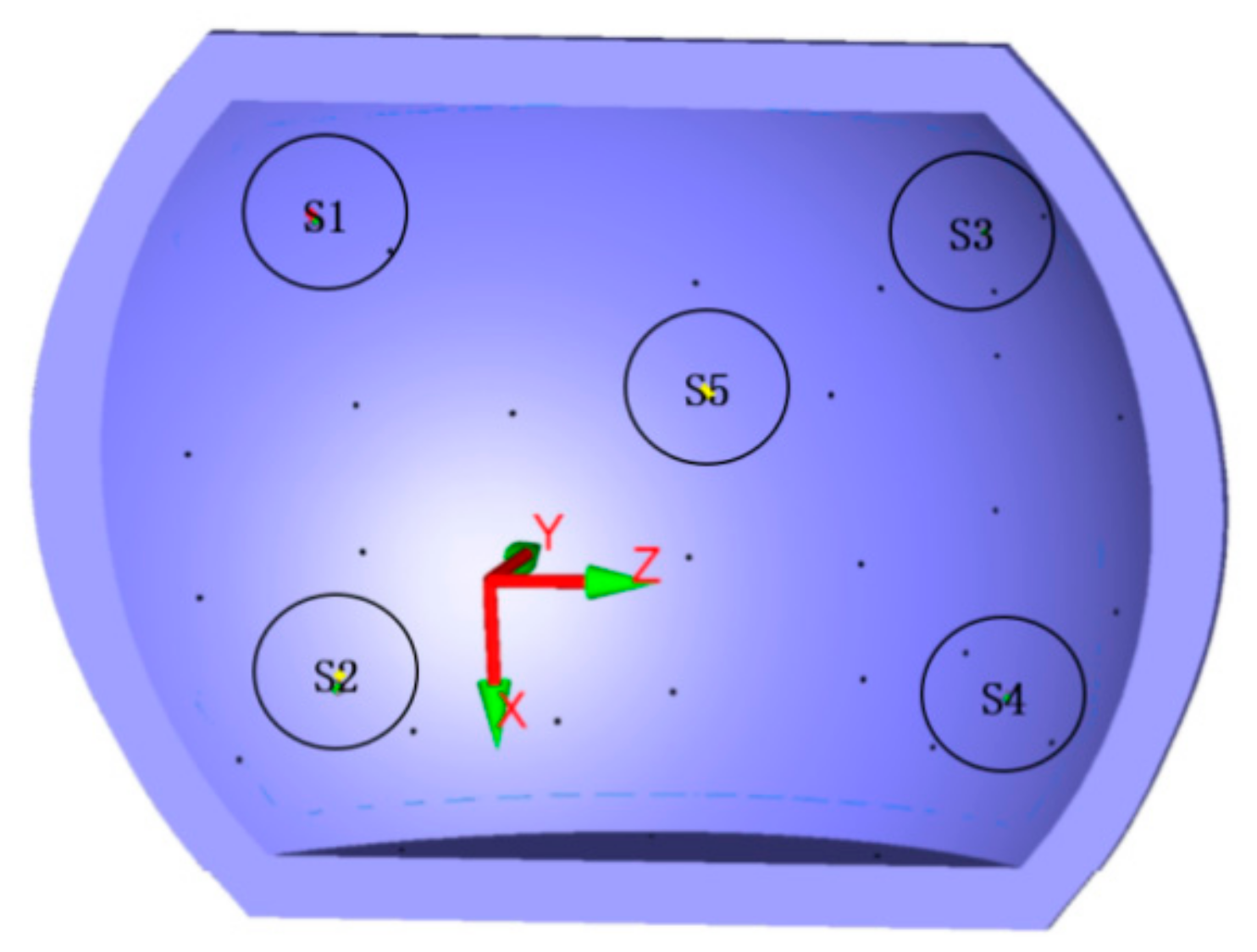
3.2. Methods
4. Results
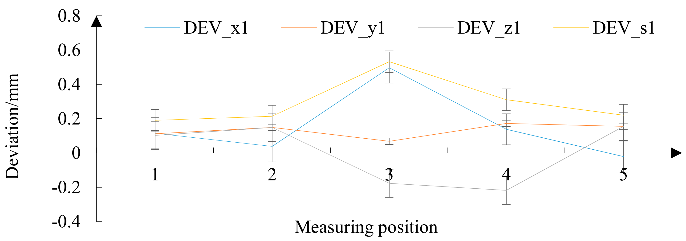
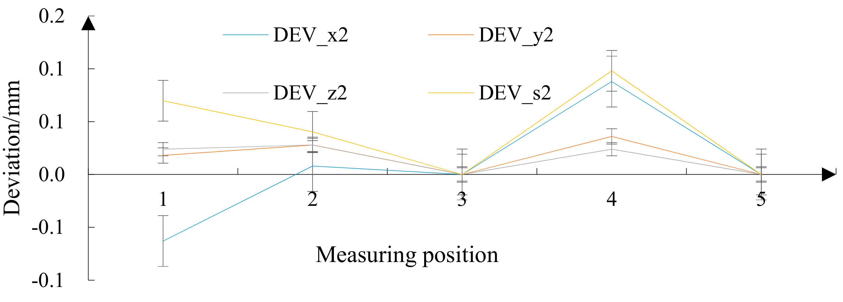
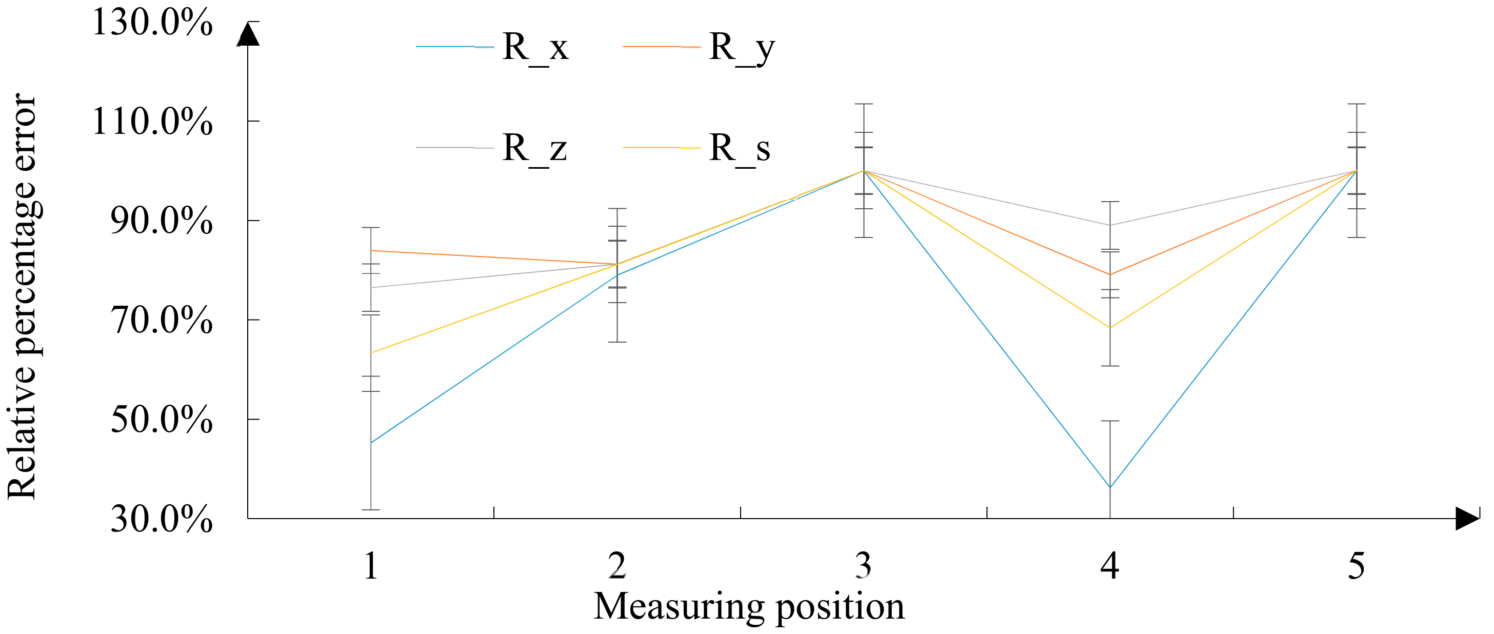
4.1. Contour Accuracy Analysis
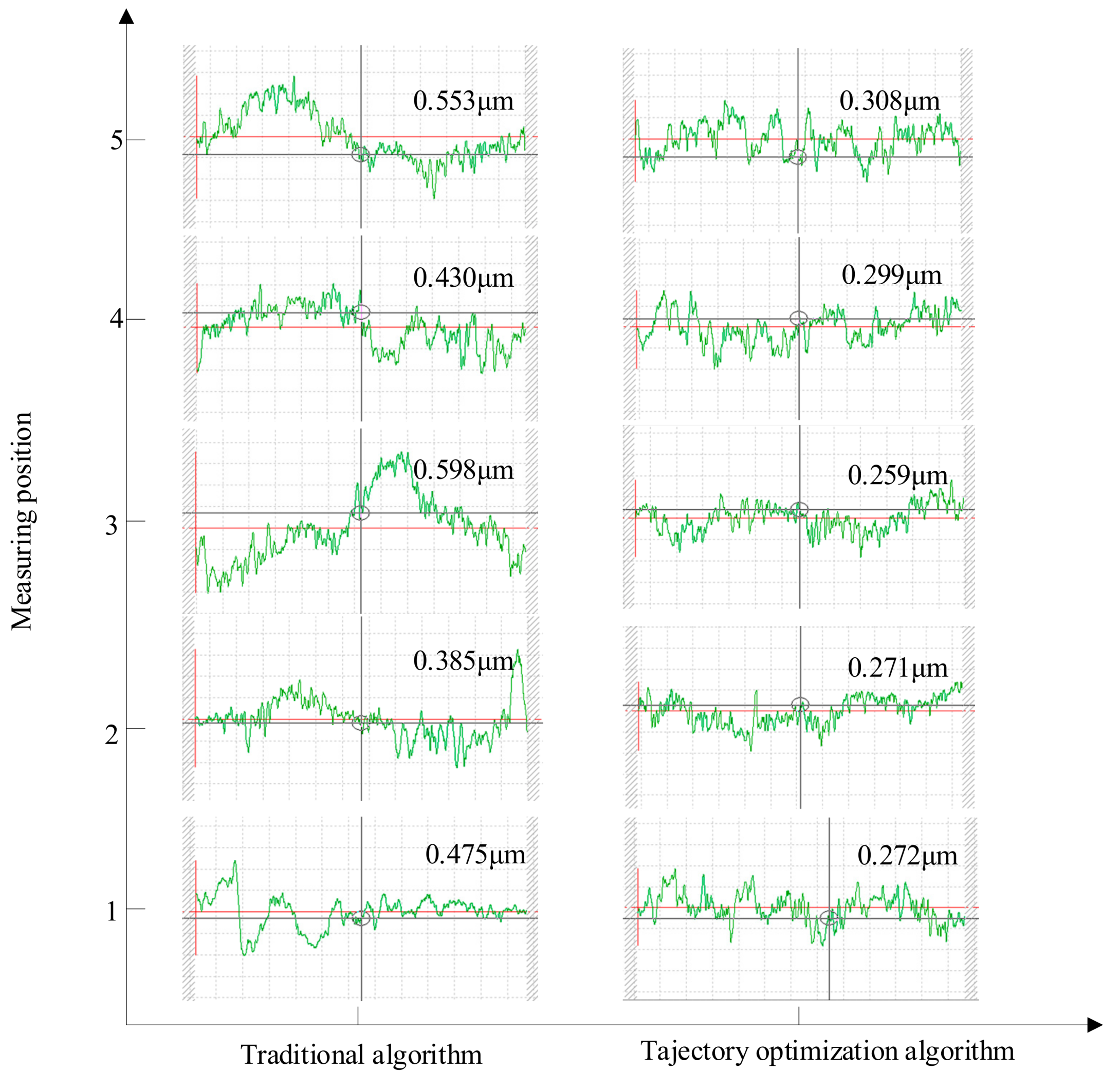
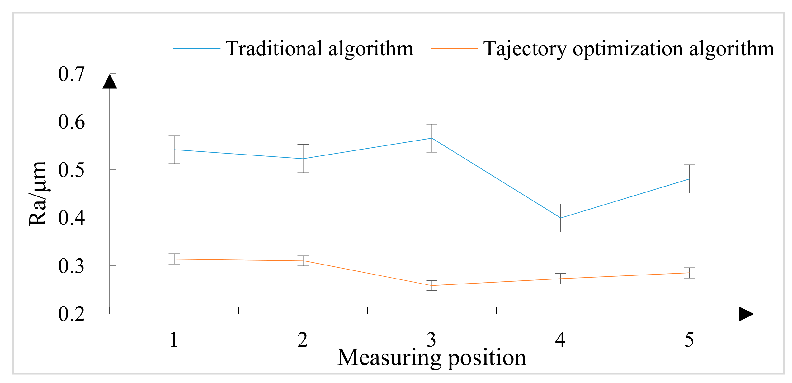
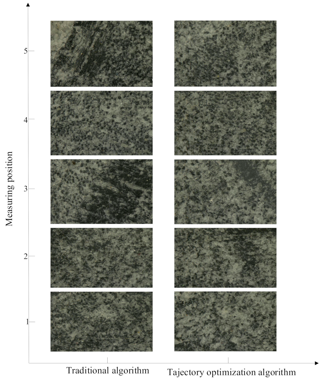
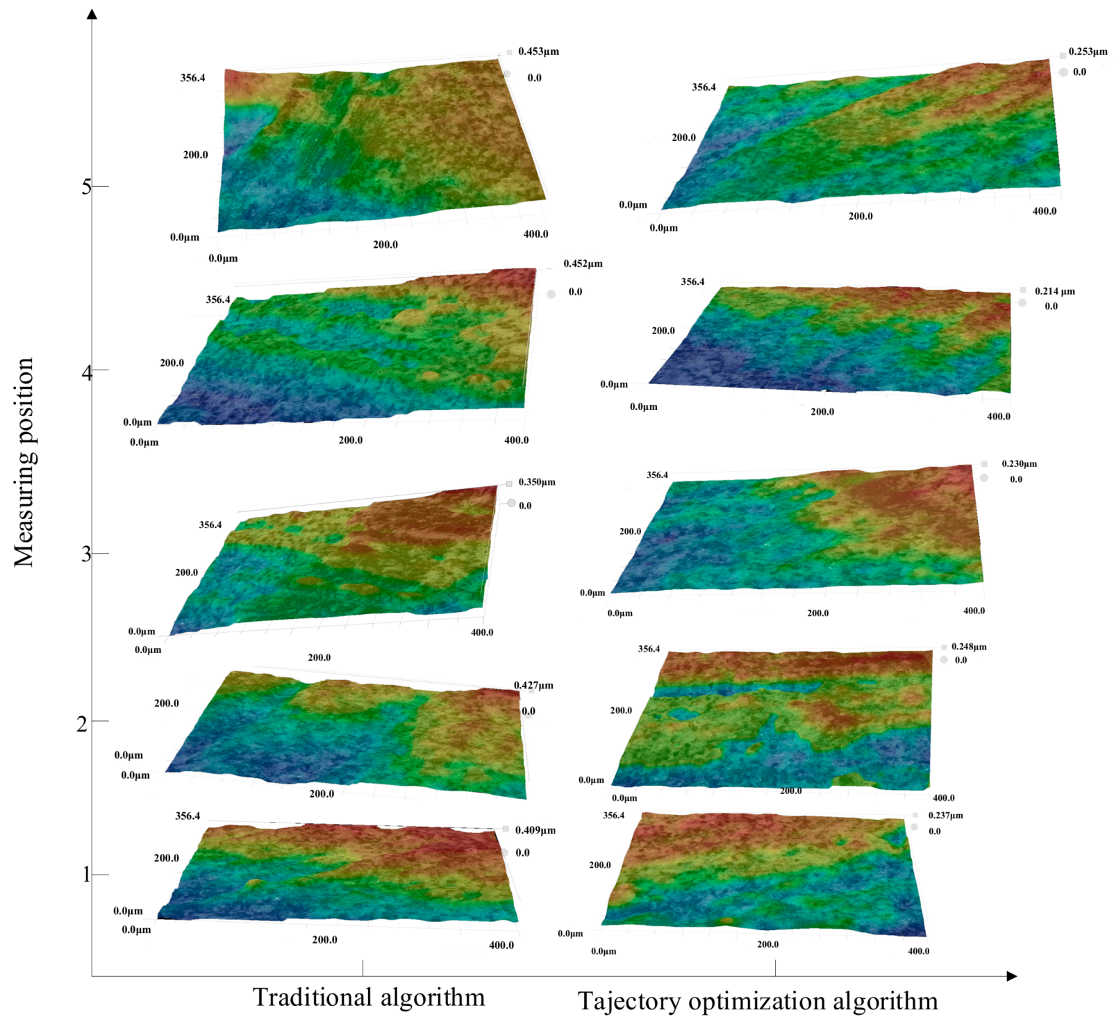
4.2. Surface Integrity
5. Conclusions
Author Contributions
Funding
Conflicts of Interest
References
- Jin, Y.M. Discussion on Drilling Holes on Connecting Edges of Radomeby Using Unilateral FRP Tooling. Fiber Reinf. Plast. 2011, 44, 1–6. [Google Scholar]
- Wang, S.Z. Development Status and Trends of Foreign FRP. FRP Compos. Mater. 1990, 6, 30–35. Available online: http://www.cnki.com.cn/Article/CJFDTotal-BLGF199006008.htm (accessed on 20 August 2019).
- Yan, S.C.; Liang, K.R. Development, Application and Prospect of FRP/Composite Materials. Guangdong Chem. Ind. 2014, 41, 72–73. [Google Scholar]
- Prasanthr, I.S.N.V.R.; Ravishankar, D.V.; Hussain, M.M.; Badiganti, C.M.; Sharma, V.K.; Pathak, S. Investigations on performance characteristics of GFRP composites in Milling. Int. J. Adv. Manuf. Technol. 2018, 99, 1351–1360. [Google Scholar] [CrossRef]
- Gemi, L.; Morkavurk, S.; Gemi, D.S.; Köklü, U. An experimental study on the effects of various drill types on drilling performance of GFRP composite pipes and damage formation. Compos. Part B 2019, 172, 186–194. [Google Scholar] [CrossRef]
- Zhang, W.S. Machining of composites. Fiber Reinf. Plast. Compos 1995, 1, 45–47. Available online: http://www.cnki.com.cn/Article/CJFDTOTAL-BLGF501.014.htm (accessed on 20 August 2019).
- Gao, C. Processing Technology of High Performance Lightweight Composite Components Used in Special Vehicle; Nanjing University of Science & Technology: Nanjing, China, 2011. [Google Scholar]
- Zhe, X. The Grinding of FRP parts. Fiber Compos. 2000, 17, 28–29. [Google Scholar]
- Huang, Y.; Huang, Z. Modern Abrasive Belt Grinding Technology and Engineering Application; Chongqing University Press: Chongqing, China, 2009. [Google Scholar]
- Xiao, G.J.; He, Y.; Huang, Y.; Li, Q. Shark-skin-inspired micro-riblets forming mechanism of TC17 titanium alloy with Belt grinding. IEEE Access. 2019. [Google Scholar] [CrossRef]
- Huo, H. Experimental Research on Milling Process of Engineering Ceramics/Glass Steel Composite Components; Nanjing University of Science & Technology: Nanjing, China, 2012. [Google Scholar]
- Hussain, S.A.; Pandurangadu, V.; Kumar, K.P. Machining parameters optimization in turning of GFRP composites by desirability function analysis embedded with Taguchi method. Int. J. Mach. Mach. Mater. 2015, 17, 95–107. [Google Scholar]
- Palanikumar, K.; Karunamoorthy, L.; Karthikeya, R. Multiple performance optimization of machining parameters on the machining of GFRP composites using carbide (K10) tool. Mater. Manuf. Process. 2006, 21, 846–852. [Google Scholar] [CrossRef]
- Vankanti, V.K.; Ganta, V. Optimization of process parameters in drilling of GFRP composite using Taguchi method. J. Mater. Res. Technol. 2014, 3, 35–41. [Google Scholar] [CrossRef]
- Solati, A.; Hamedi, M.; Safarabadi, M. Combined GA-ANN approach for prediction of HAZ and bearing strength in laser drilling of GFRP composite. Opt. Laser Technol. 2019, 113, 104–115. [Google Scholar] [CrossRef]
- Shi, K.N.; Ren, J.X.; Wang, S.B.; Liu, N.; Liu, Z.M.; Zhang, D.H.; Lu, W.F. An Improved Cutting Power-based Model for Evaluating Total Energy Consumption in General End. Milling Process J. Clean. Prod. 2019, 231, 1330–1341. [Google Scholar] [CrossRef]
- Wang, R.; Wang, Y.; Wu, C.K.; Li, L. Research of the Method for FRP Yacht Surface Modeling Based on the High Dimensional Data. Ship Eng. 2012, 34, 154–157. [Google Scholar]
- Oqielat, M.N. Surface fitting methods for modelling leaf surface from scanned data. J. King Saud Univ. Sci. 2019, 31. [Google Scholar] [CrossRef]


| Number | Relative Position X | Relative Position Y | Number | Relative Position X | Relative Position Y |
|---|---|---|---|---|---|
| 1 | 82.943 | −23.279 | 24 | −3.8173 | 12.385 |
| 2 | 79.795 | −20.676 | 25 | −7.6255 | 12.187 |
| 3 | 76.646 | −18.073 | 26 | −11.424 | 11.858 |
| 4 | 73.498 | −15.469 | 27 | −15.21 | 11.398 |
| 5 | 67.369 | −10.487 | 28 | −18.977 | 10.807 |
| 6 | 64.308 | −8.2131 | 29 | −22.722 | 10.087 |
| 7 | 61.171 | −6.0457 | 30 | −26.439 | 9.2382 |
| 8 | 57.961 | −3.9879 | 31 | −30.125 | 8.2612 |
| 9 | 54.681 | −2.0422 | 32 | −33.775 | 7.1574 |
| 10 | 51.336 | −0.211 | 33 | −37.385 | 5.9282 |
| 11 | 47.93 | 1.5037 | 34 | −40.95 | 4.5751 |
| 12 | 44.467 | 3.0997 | 35 | −44.467 | 3.0997 |
| 13 | 40.95 | 4.5751 | 36 | −47.93 | 1.5037 |
| 14 | 37.385 | 5.9282 | 37 | −51.336 | −0.211 |
| 15 | 33.775 | 7.1574 | 38 | −54.681 | −2.0422 |
| 16 | 30.125 | 8.2612 | 39 | −57.96 | −3.9879 |
| 17 | 26.439 | 9.2382 | 40 | −61.171 | −6.0457 |
| 18 | 22.722 | 10.087 | 41 | −64.308 | −8.2131 |
| 19 | 18.977 | 10.807 | 42 | −67.369 | −10.487 |
| 20 | 15.21 | 11.398 | 43 | −73.498 | −15.469 |
| 21 | 11.424 | 11.852 | 44 | −76.646 | −18.073 |
| 22 | 7.6256 | 12.187 | 45 | −79.795 | −20.676 |
| 23 | 3.8174 | 12.385 | 46 | −82.943 | −23.279 |
| Number | Relative Position X | Relative Position Y | Number | Relative Position X | Relative Position Y |
|---|---|---|---|---|---|
| 1 | −84.123 | −23.829 | 20 | −3.817 | 12.385 |
| 2 | −80.188 | −20.466 | 21 | −7.625 | 12.187 |
| 3 | −76.252 | −17.265 | 22 | −11.424 | 11.858 |
| 4 | −72.317 | −14.225 | 23 | −15.213 | 11.398 |
| 5 | −68.353 | −11.325 | 24 | −18.977 | 10.807 |
| 6 | −64.291 | −8.523 | 25 | −22.722 | 10.087 |
| 7 | −60.093 | −5.808 | 26 | −26.439 | 9.238 |
| 8 | −55.767 | −3.201 | 27 | −30.125 | 8.261 |
| 9 | −51.322 | −0.726 | 28 | −33.775 | 7.157 |
| 10 | −46.769 | 1.595 | 29 | −37.385 | 5.928 |
| 11 | −42.117 | 3.746 | 30 | −40.953 | 4.575 |
| 12 | −37.375 | 5.706 | 31 | −44.467 | 3.099 |
| 13 | −32.554 | 7.459 | 32 | −47.935 | 1.503 |
| 14 | −27.664 | 8.990 | 33 | −51.336 | −0.211 |
| 15 | −22.715 | 10.286 | 34 | −54.681 | −2.042 |
| 16 | −17.719 | 11.337 | 35 | −57.962 | −3.987 |
| 17 | −12.684 | 12.133 | 36 | −61.171 | −6.045 |
| 18 | −7.623 | 12.667 | 37 | −64.308 | −8.213 |
| 19 | −2.545 | 12.936 | 38 | −67.369 | −10.487 |
| Parameter | Range |
|---|---|
| Turntable diameter (mm) | 1500 |
| Turntable speed (r/min) frequency conversion adjustable | 1–20 |
| Processing barrel and head diameter (mm) | Φ800–Φ4000 |
| Throwing efficiency (/h) | 6–10 |
| Surface roughness, Ra (μm) | 0.1–0.4 |
| Contact wheel size (mm) | Φ25–Φ180 |
| x/y/z-axis repeat positioning accuracy | ≤0.01 mm |
| Surface Average Roughness | |
|---|---|
| Traditional algorithm | 0.503 μm |
| Trajectory optimization algorithm | 0.289 μm |
© 2019 by the authors. Licensee MDPI, Basel, Switzerland. This article is an open access article distributed under the terms and conditions of the Creative Commons Attribution (CC BY) license (http://creativecommons.org/licenses/by/4.0/).
Share and Cite
Xing, J.; Xiao, G.; He, Y.; Huang, Y.; Liu, S. The Fitting of a Fiber-Reinforced-Plastic Complex Curved Surface and Its Orbit Optimization Model with Belt Grinding Line Contact. Materials 2019, 12, 2688. https://doi.org/10.3390/ma12172688
Xing J, Xiao G, He Y, Huang Y, Liu S. The Fitting of a Fiber-Reinforced-Plastic Complex Curved Surface and Its Orbit Optimization Model with Belt Grinding Line Contact. Materials. 2019; 12(17):2688. https://doi.org/10.3390/ma12172688
Chicago/Turabian StyleXing, Jiazheng, Guijian Xiao, Yi He, Yun Huang, and Shuai Liu. 2019. "The Fitting of a Fiber-Reinforced-Plastic Complex Curved Surface and Its Orbit Optimization Model with Belt Grinding Line Contact" Materials 12, no. 17: 2688. https://doi.org/10.3390/ma12172688
APA StyleXing, J., Xiao, G., He, Y., Huang, Y., & Liu, S. (2019). The Fitting of a Fiber-Reinforced-Plastic Complex Curved Surface and Its Orbit Optimization Model with Belt Grinding Line Contact. Materials, 12(17), 2688. https://doi.org/10.3390/ma12172688