Comparative Study on Constitutive Models for 21-4N Heat Resistant Steel during High Temperature Deformation


 ,
,
Abstract
1. Introduction
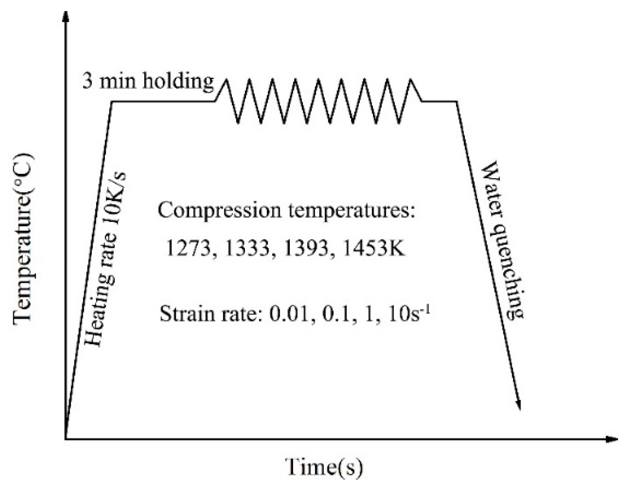
2. Experiment
3. Result and Discussion
3.1. J-C Model
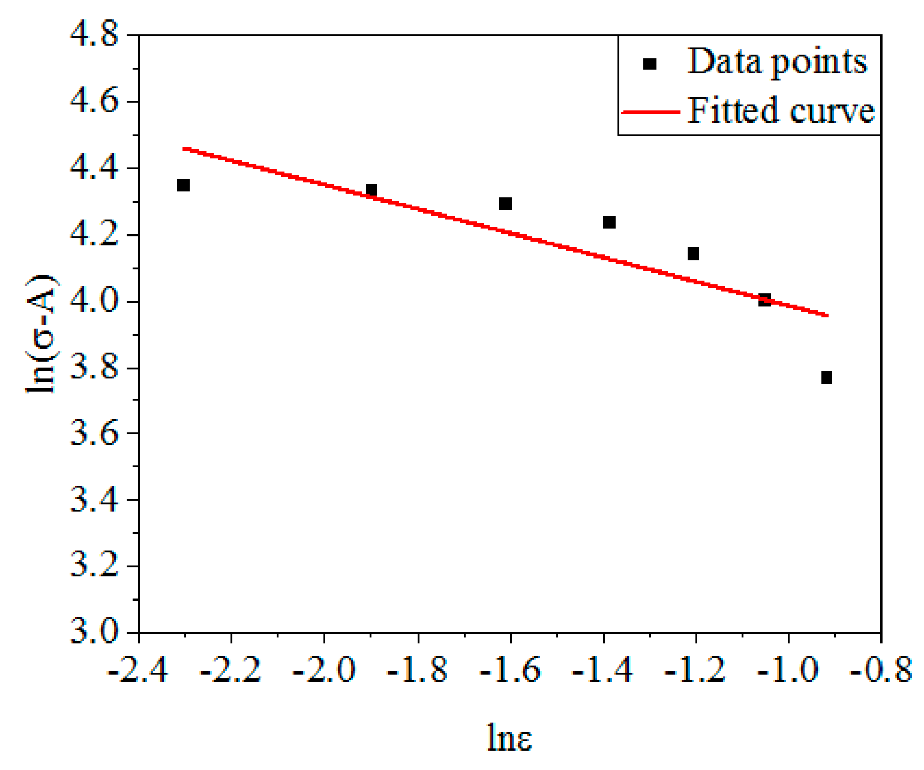
3.1.1. Determination of Parameters n and B
3.1.2. Determination of Parameter C
3.1.3. Determination of Parameter m
3.2. Modified J-C Model
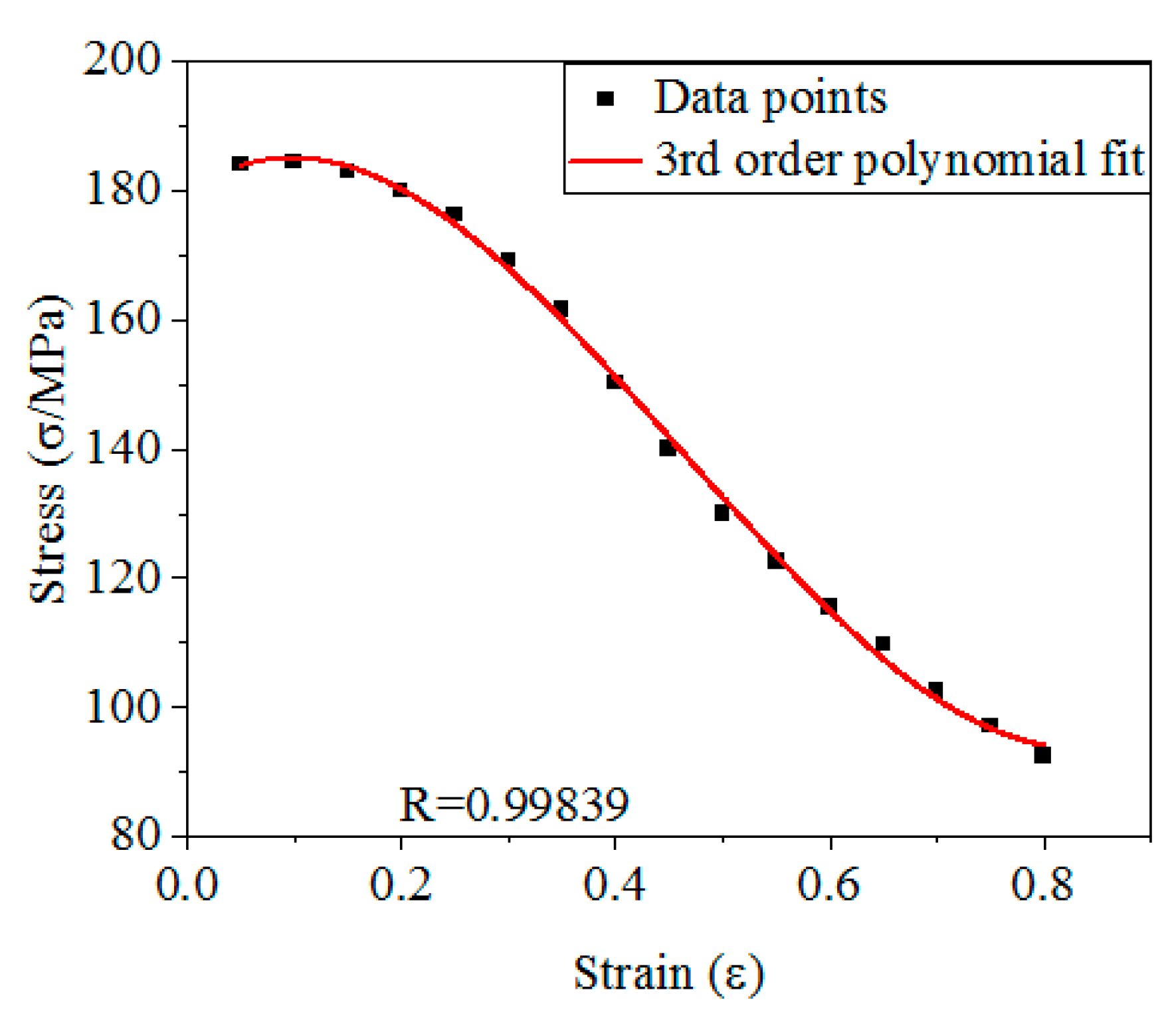
3.2.1. Determination of Parameters A1, B1, B2, B3
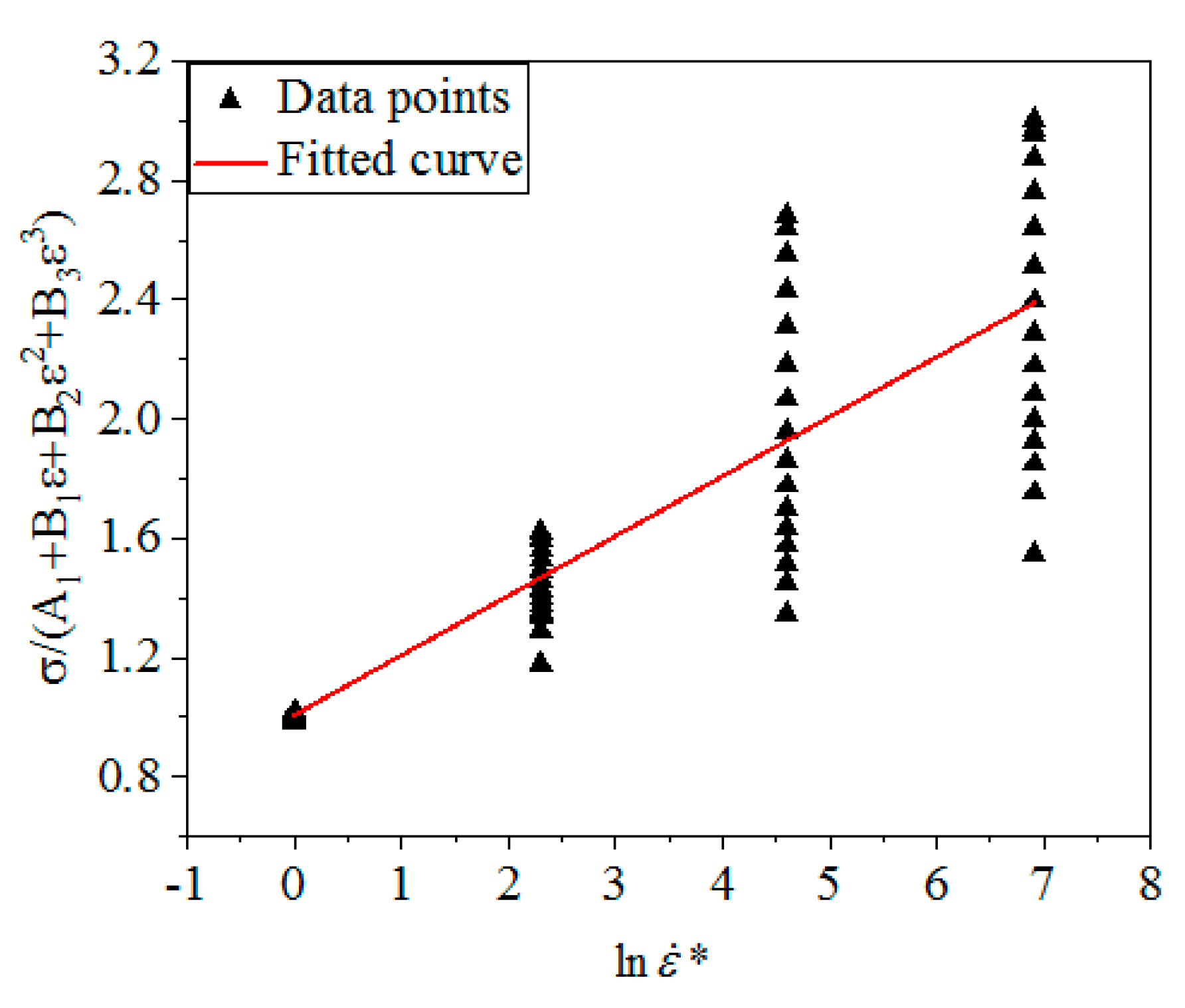
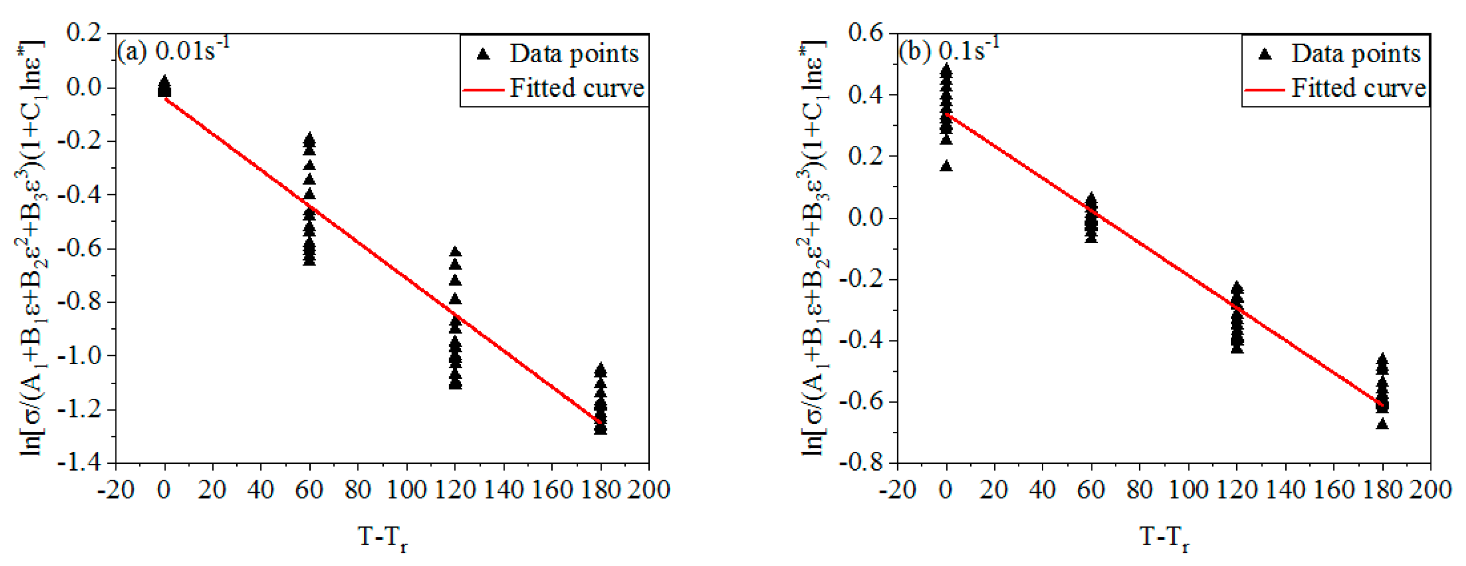
3.2.2. Determination of Parameter C1
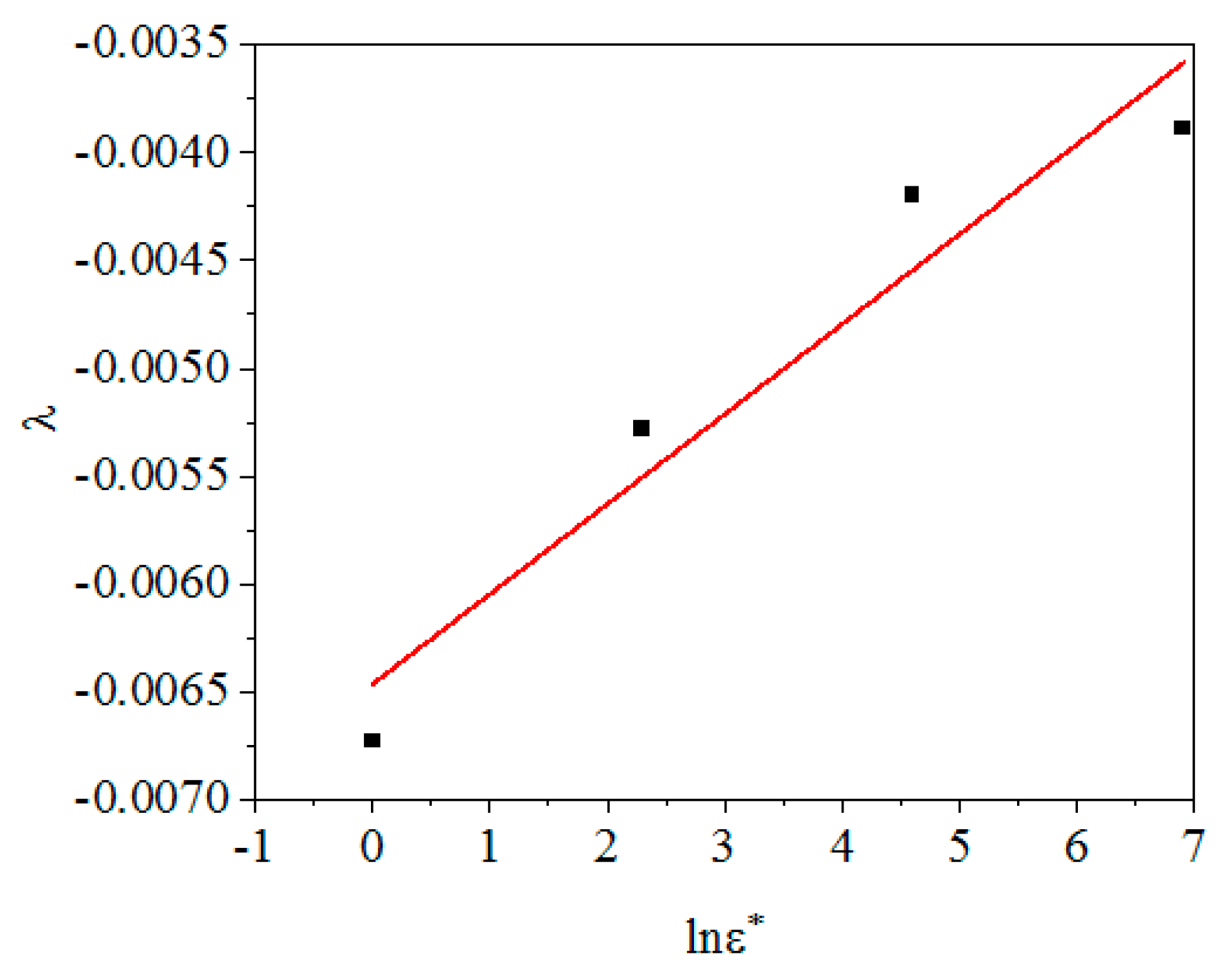
3.2.3. Determination of Parameters λ1, λ2
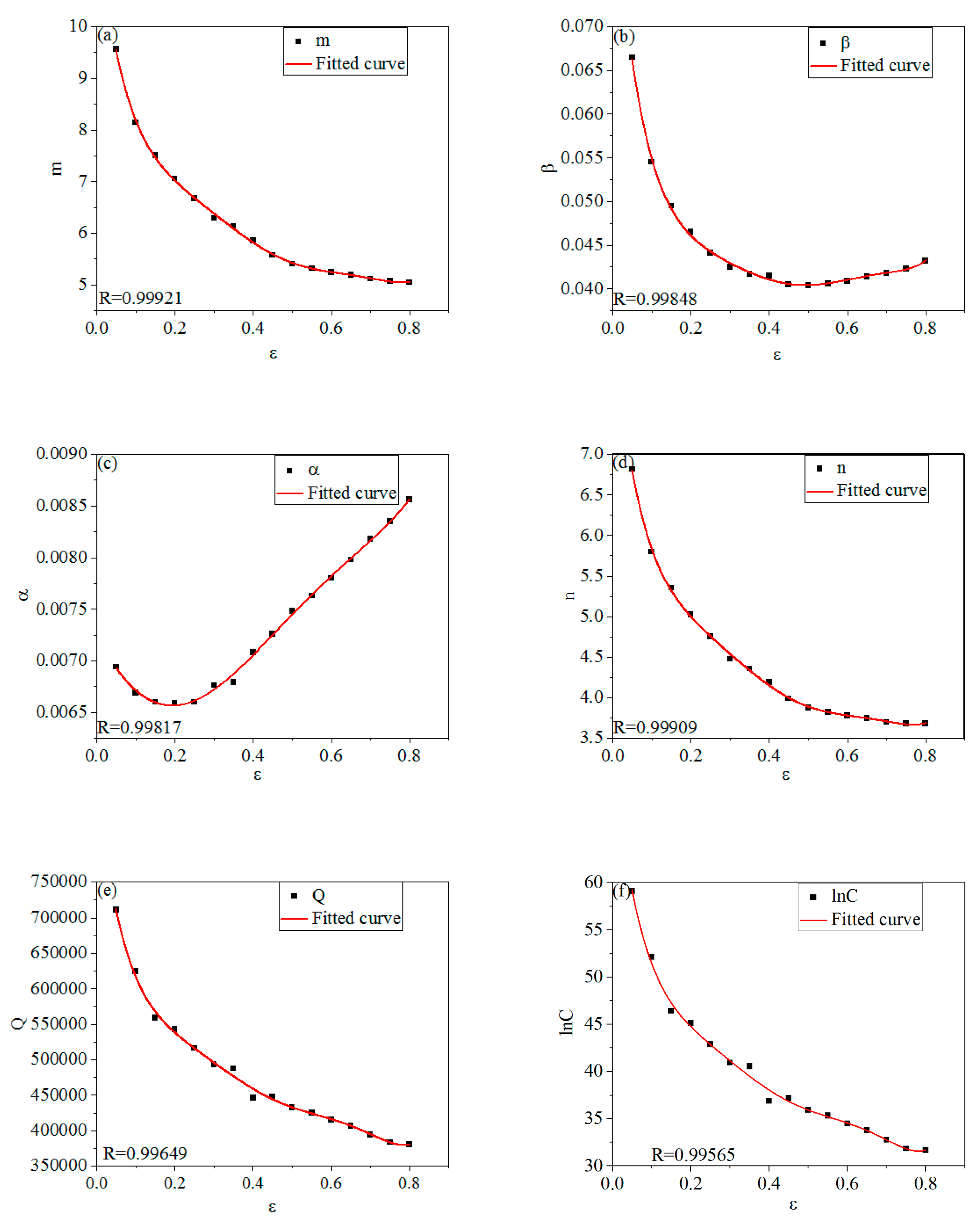
3.3. Arrhenius Model
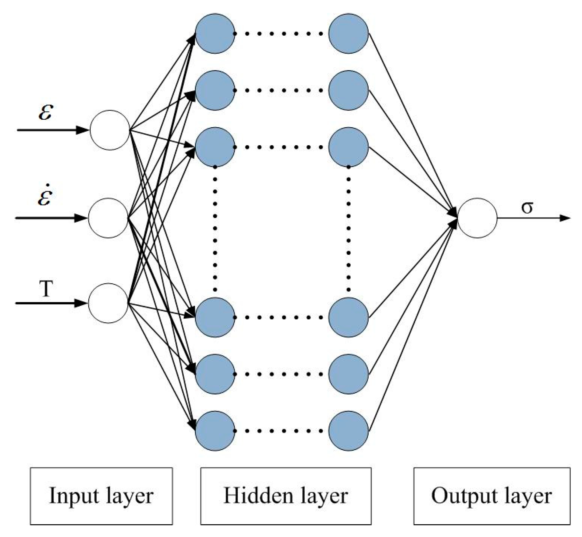
3.4. BP-ANN Model
3.5. Analysis of Constitutive Equation Accuracy
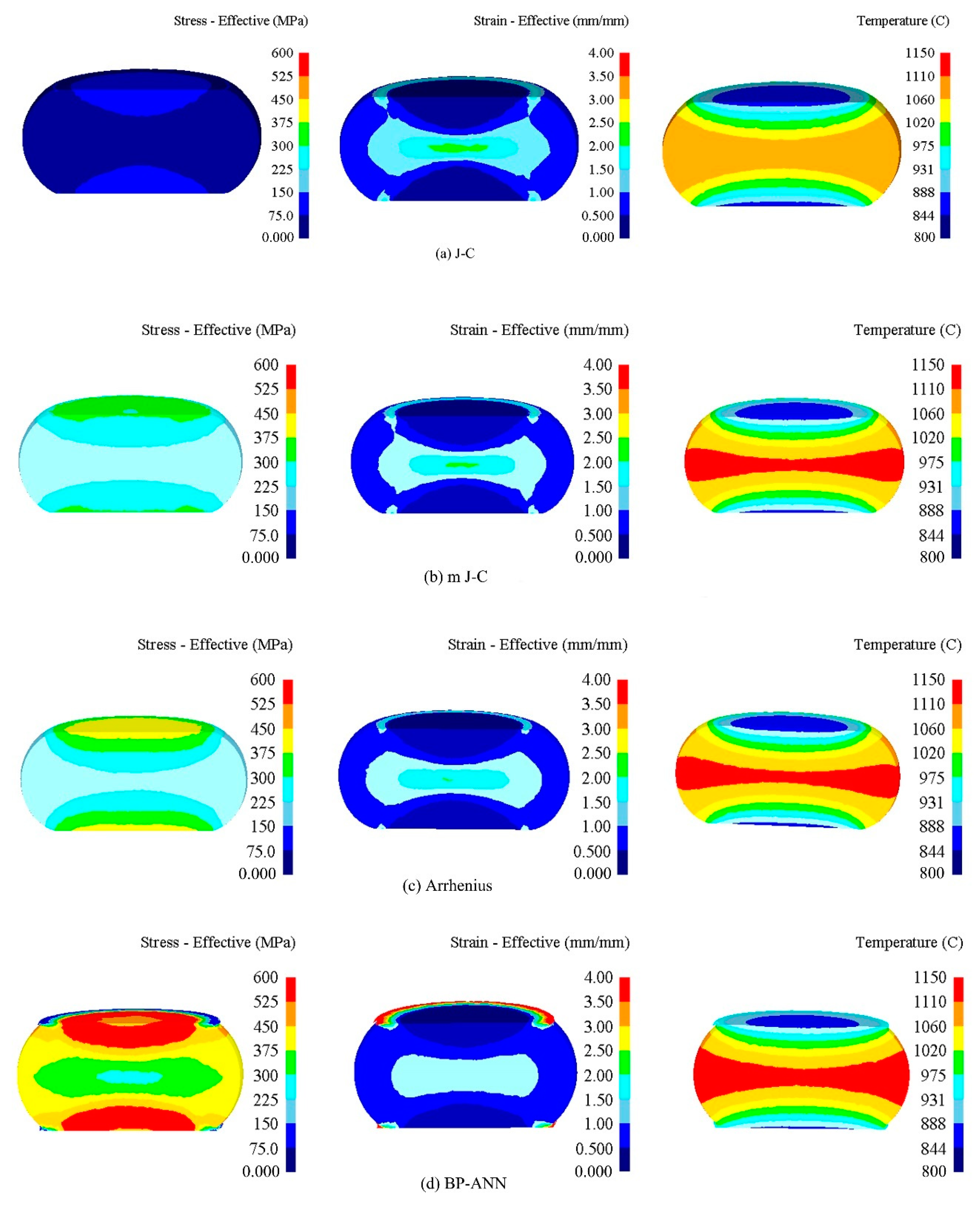
3.6. Finite Element Simulation of Four Models
4. Conclusions
- The T and are the main influencing factors of 21-4N during hot deformation, and they have a coupling effect on σ.
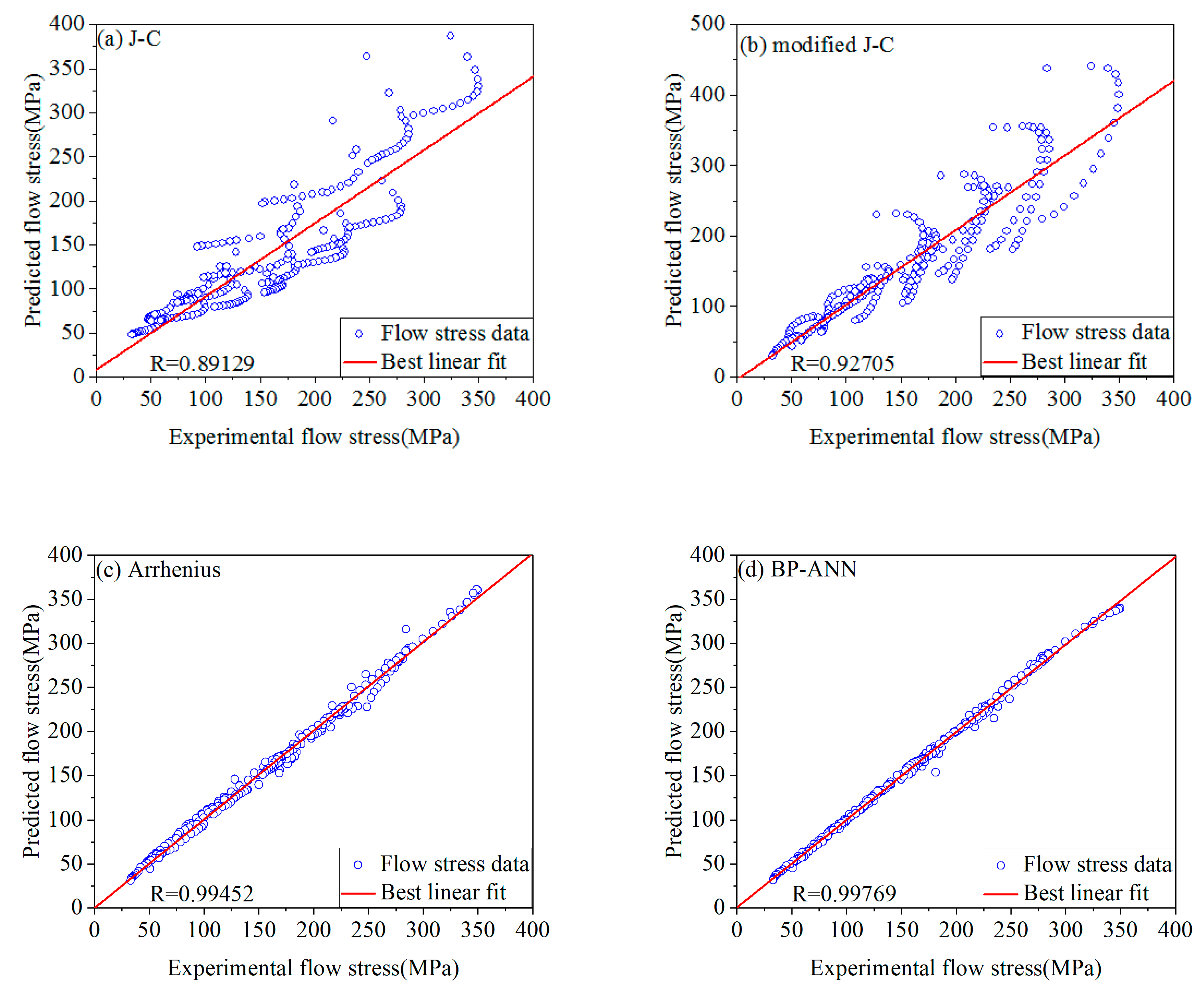
- J-C model ignores the coupling effect of the and T. As a result, when the deformation condition changes greatly, the accuracy decreases obviously.
- Modified J-C model considers the coupling effect of T and . The parameter compensation is carried out on the basis of J-C model. The prediction accuracy has been greatly improved. When the deformation condition changes greatly, the accuracy of it is still within a reasonable range.
- Arrhenius model uses the Z parameter to express the coupling effect of T and . The prediction accuracy is higher than modified J-C model. It is suitable for the σ prediction under the reasonable deformation conditions.
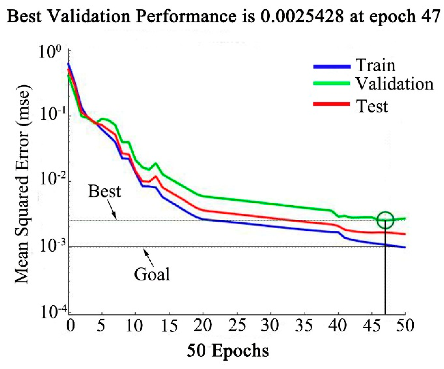
- The established BP-ANN model has two hidden layers, which is 3 × 10 × 10 × 1 topology, and the training is completed after 47 iterations. And it has a very high accuracy under the conditions allowed by the deformation conditions.
- All the four models can be input into the finite element software for compression test simulation, and the simulation results are not much different from the experimental results, indicating that the four models established have certain practicability.
Author Contributions
Funding
Conflicts of Interest
References
- Ji, H.C.; Liu, J.P.; Wang, B.Y.; Tang, X.F.; Lin, J.G.; Huo, Y.M. Microstructure evolution and constitutive equations for the high-temperature deformation of 5Cr21Mn9Ni4N heat-resistant steel. J. Alloys Compd. 2017, 693, 674–687. [Google Scholar] [CrossRef]
- Li, W.Y.; Yu, M.; Li, J.L.; Zhang, G.F.; Wang, S.Y. Characterizations of 21-4N to 4Cr9Si2 stainless steel dissimilar joint bonded by electric-resistance-heat-aided friction welding. Mater. Des. 2009, 30, 4230–4235. [Google Scholar] [CrossRef]
- Ji, H.C.; Li, Y.M.; Ma, C.J.; Long, H.Y.; Liu, J.P.; Wang, B.Y. Modeling of austenitic grain growth of 21-4N steel. Metalurgija 2019, 58, 83–86. [Google Scholar]
- Changizian, P.; Zarei-Hanzaki, A.; Roostaei, A.A. The high temperature flow behavior modeling of AZ81 magnesium alloy considering strain effects. Mater. Des. 2012, 39, 384–389. [Google Scholar] [CrossRef]
- Lee, J.W.; Son, H.W.; Hyun, S.K. Hot deformation behavior of AA6005 modified with CaO-added Mg at high strains. J. Alloys Compd. 2019, 774, 1081–1091. [Google Scholar] [CrossRef]
- Cui, C.P.; Gao, Y.M.; Wei, S.Z.; Zhang, G.S.; Zhou, Y.C.; Zhu, X.W. Microstructure and high temperature deformation behavior of the Mo-ZrO2, alloys. J. Alloys Compd. 2017, 716, 321–329. [Google Scholar] [CrossRef]
- Qin, Y.J.; Pan, Q.L.; He, Y.B.; Li, W.B.; Liu, X.Y.; Fan, X. Modeling of flow stress for magnesium alloy during hot deformation. Mater. Sci. Eng. A 2010, 527, 2790–2797. [Google Scholar] [CrossRef]
- Bennett, C.J. A comparison of material models for the numerical simulation of spike-forging of a CrMoV alloy steel. Comput. Mater. Sci. 2013, 70, 114–122. [Google Scholar] [CrossRef]
- Cai, Z.M.; Ji, H.C.; Pei, W.C.; Tang, X.F.; Huang, X.M.; Liu, J.P. Hot workability, constitutive model and processing map of 3Cr23Ni8Mn3N heat resistant steel. Vacuum 2019, 165, 324–336. [Google Scholar] [CrossRef]
- Ma, A.; Roters, F.; Raabe, D. A dislocation density based constitutive model for crystal plasticity FEM including geometrically necessary dislocations. Acta Mater. 2006, 54, 2169–2179. [Google Scholar] [CrossRef]
- Thakur, N.; Kumar, P.; Bharj, R.S. Effect of variation of Johnson-Cook parameters on kinetic energy and simulation of 4340 steel projectile. Mater. Today Proc. 2018, 5, 27884–27892. [Google Scholar] [CrossRef]
- Karkalos, N.E.; Markopoulos, A.P. Determination of Johnson-Cook material model parameters by an optimization approach using the fireworks algorithm. Procedia Manuf. 2018, 22, 107–113. [Google Scholar] [CrossRef]
- Sahu, S.; Mondal, D.P.; Goel, M.D.; Ansari, M.Z. Finite element analysis of AA1100 elasto-plastic behaviour using Johnson-Cook model. Mater. Today Proc. 2018, 5, 5349–5353. [Google Scholar] [CrossRef]
- Limbadri, K.; Toshniwal, K.; Suresh, K.; Gupta, A.K.; Rao, K.V.V.; Ram, M.; Ravindran, M.; Kalyankrishnan, G.; Singh, S.K. Stress variation of Zircaloy-4 and Johnson Cook model for rolled sheets. Mater. Today Proc. 2018, 5, 3793–3801. [Google Scholar] [CrossRef]
- Limbadri, K.; Krishnamurthy, H.N.; Ram, M.A.; Saibaba, N.; Rao, K.V.V.; Murthy, J.N.; Gupta, A.K.; Singh, S.K. Development of Johnson Cook model for Zircaloy-4 with Low Oxygen Content. Mater. Today Proc. 2017, 4, 966–974. [Google Scholar] [CrossRef]
- Buzyurkin, A.E.; Gladky, I.L.; Kraus, E.I. Determination and verification of Johnson-Cook model parameters at high-speed deformation of titanium alloys. Aerosp. Sci. Technol. 2015, 45, 121–127. [Google Scholar] [CrossRef]
- Jia, C.L.; Chen, F.R. Finite element simulation of Johnson-Cook constitutive model for 7A52 aluminum alloy. Ordnance Mater. Sci. Eng. 2018, 41, 30–33. [Google Scholar]
- Wang, F.Z.; Zhao, J.; Zhu, N.B.; Li, Z.L. A comparative study on Johnson-Cook constitutive modeling for Ti-6Al-4V alloy using automated ball indentation (ABI) technique. J. Alloys Compd. 2015, 633, 220–228. [Google Scholar] [CrossRef]
- Grzesik, W.; Nieslony, P.; Laskowski, P. Determination of Material Constitutive Laws for Inconel 718 Superalloy Under Different Strain Rates and Working Temperatures. J. Mater. Eng. Perform. 2017, 26, 5705–5714. [Google Scholar] [CrossRef]
- Tuğrul, Ö.; Yiğit, K. Identification of Constitutive Material Model Parameters for High-Strain Rate Metal Cutting Conditions Using Evolutionary Computational Algorithms. Adv. Manuf. Process. 2007, 22, 659–667. [Google Scholar]
- Zhao, Y.H.; Sun, J.; Li, J.F.; Yan, Y.Q.; Wang, P. A comparative study on Johnson-Cook and modified Johnson-Cook constitutive material model to predict the dynamic behavior laser additive manufacturing FeCr alloy. J. Alloys Compd. 2017, 723, 179–187. [Google Scholar] [CrossRef]
- Zhang, D.N.; Shangguan, Q.Q.; Xie, C.J.; Liu, F. A modified Johnson-Cook model of dynamic tensile behaviors for 7075-T6 aluminum alloy. J. Alloys Compd. 2015, 619, 186–194. [Google Scholar] [CrossRef]
- Tan, J.Q.; Zhan, M.; Liu, S.; Huang, T.; Guo, J.; Yang, H. A modified Johnson-Cook model for tensile flow behaviors of 7050-T7451 aluminum alloy at high strain rates. Mater. Sci. Eng. A 2015, 631, 214–219. [Google Scholar] [CrossRef]
- Wang, X.Y.; Huang, C.Z.; Zou, B.; Liu, H.L.; Zhu, H.T.; Wang, J. Dynamic behavior and a modified Johnson-Cook constitutive model of Inconel 718 at high strain rate and elevated temperature. Mater. Sci. Eng. A 2013, 580, 385–390. [Google Scholar] [CrossRef]
- Bobbili, R.; Madhu, V. Constitutive modeling and fracture behavior of a biomedical Ti-13Nb-13Zr alloy. Mater. Sci. Eng. A 2017, 700, 82–91. [Google Scholar] [CrossRef]
- Prawoto, Y.; Fanone, M.; Shahedi, S.; Ismail, M.S.; Wan-Nik, W.B. Computational approach using Johnson-Cook model on dual phase steel. Comput. Mater. Sci. 2012, 54, 48–55. [Google Scholar] [CrossRef]
- Ducobu, F.; Rivière-Lorphèvre, E.; Filippi, E. On the importance of the choice of the parameters of the Johnson-Cook constitutive model and their influence on the results of a Ti6Al4V orthogonal cutting model. Int. J. Mech. Sci. 2017, 122, 143–155. [Google Scholar] [CrossRef]
- Ranc, N.; Chrysochoos, A. Calorimetric consequences of thermal softening in Johnson-Cook’s model. Mech. Mater. 2013, 65, 44–55. [Google Scholar] [CrossRef]
- Shrot, A.; BäKer, M. Determination of Johnson-Cook parameters from machining simulations. Comput. Mater. Sci. 2012, 52, 298–304. [Google Scholar] [CrossRef]
- He, J.L.; Chen, F.; Wang, B.; Zhu, L.B. A modified Johnson-Cook model for 10%Cr steel at elevated temperatures and a wide range of strain rates. Mater. Sci. Eng. A 2018, 715, 1–9. [Google Scholar] [CrossRef]
- Chen, G.; Chen, W.; Ma, L.; Guo, A.Z.; Lü, J.; Zhang, Z.M.; Zheng, S.Q. Strain-Compensated Arrhenius-type constitutive model for flow behavior of Al-12Zn-2.4Mg-1.2Cu alloy. Rare Met. Mater. Eng. 2015, 44, 2120–2125. [Google Scholar]
- Abbasi-Bani, A.; Zarei-Hanzaki, A.; Pishbin, M.H.; Haghdadi, N. A comparative study on the capability of Johnson-Cook and Arrhenius-type constitutive equations to describe the flow behavior of Mg-6Al-1Zn alloy. Mech. Mater. 2014, 71, 52–61. [Google Scholar] [CrossRef]
- Li, Y.F.; Wang, Z.H.; Zhang, L.Y.; Luo, C.; Lai, X.C. Arrhenius-type constitutive model and dynamic recrystallization behavior of V-5Cr-5Ti alloy during hot compression. Trans. Nonferrous Met. Soc. China 2015, 25, 1889–1900. [Google Scholar] [CrossRef]
- Quan, G.Z.; Wang, B.; Liu, J.F.; Zhang, Y.W. Study on variable parameter Arrhenius model of thermal compression stress-strain relationship of extruded 42CrMo steel. Hot Work. Technol. 2016, 45, 104–107. [Google Scholar]
- Quan, G.Z.; Zhang, Y.W.; Chen, T.; Zhou, J.; Liu, D.J. Characterization of thermoplastic flow behavior for Ti-6Al-2Zr-1Mo-1V alloy by Arrhenius model with variable parameters. J. Funct. Mater. 2012, 5, 545–549. [Google Scholar]
- Samantaray, D.; Mandal, S.; Bhaduri, A.K. A comparative study on Johnson Cook, modified Zerilli-Armstrong and Arrhenius-type constitutive models to predict elevated temperature flow behaviour in modified 9Cr-1Mo steel. Comput. Mater. Sci. 2009, 47, 568–576. [Google Scholar] [CrossRef]
- Li, J.; Li, F.G.; Cai, J.; Wang, R.T.; Yuan, Z.W.; Ji, G.L. Comparative investigation on the modified Zerilli-Armstrong model and Arrhenius-type model to predict the elevated-temperature flow behaviour of 7050 aluminium alloy. Comput. Mater. Sci. 2013, 71, 56–65. [Google Scholar] [CrossRef]
- Yan, G.X.; Crivoi, A.; Sun, Y.J.; Maharjan, N.; Song, X.; Li, F.; Tan, M.J. An Arrhenius equation-based model to predict the residual stress relief of post weld heat treatment of Ti-6Al-4V plate. J. Manuf. Process. 2018, 32, 763–772. [Google Scholar] [CrossRef]
- Li, H.Y.; Li, Y.H.; Wang, X.F.; Liu, J.J.; Wu, Y. A comparative study on modified Johnson Cook, modified Zerilli-Armstrong and Arrhenius-type constitutive models to predict the hot deformation behavior in 28CrMnMoV steel. Mater. Des. 2013, 49, 493–501. [Google Scholar] [CrossRef]
- Yan, J.; Pan, Q.L.; Song, W.B. Flow behavior of Al-6.2Zn-0.70Mg-0.30Mn-0.17Zr alloy during hot compressive deformation based on Arrhenius and ANN model. Trans. Nonferrous Met. Soc. China 2017, 27, 638–647. [Google Scholar] [CrossRef]
- Han, Y.; Qiao, G.J.; Sun, J.P.; Zou, D.N. A comparative study on constitutive relationship of as-cast 904L austenitic stainless steel during hot deformation based on Arrhenius-type and artificial neural network models. Comput. Mater. Sci. 2013, 67, 93–103. [Google Scholar] [CrossRef]
- Peng, W.W.; Zeng, W.D.; Wang, Q.J.; Yu, H.Q. Comparative study on constitutive relationship of as-cast Ti60 titanium alloy during hot deformation based on Arrhenius-type and artificial neural network models. Mater. Des. 2013, 51, 95–104. [Google Scholar] [CrossRef]
- Vignesh, R.V.; Padmanaban, R. Artificial neural network model for predicting the tensile strength of friction stir welded aluminium alloy AA1100. Mater. Today Proc. 2018, 5, 16716–16723. [Google Scholar] [CrossRef]
- Ji, H.C.; Huang, X.M.; Ma, C.J.; Pei, W.C.; Liu, J.P.; Wang, B.Y. Predicting the microstructure of a valve head during the hot forging of steel 21-4N. Metals 2018, 8, 391. [Google Scholar] [CrossRef]
- Li, Y.M.; Ji, H.C.; Li, W.D.; Li, Y.G.; Pei, W.C.; Liu, J.P. Hot Deformation characteristics-constitutive equation and processing maps-of 21-4N heat-resistant steel. Materials 2019, 12, 89. [Google Scholar] [CrossRef] [PubMed]
- Johnson, G.R.; Cook, W.H. Fracture characteristics of three metals subjected to various strains, strain rates, temperatures and pressures. Eng. Fract. Mech. 1985, 21, 31–48. [Google Scholar] [CrossRef]
- Schulze, V.; Zanger, F. Numerical Analysis of the influence of Johnson-Cook-Material parameters on the surface integrity of Ti-6Al-4 V. Procedia Eng. 2011, 19, 306–311. [Google Scholar] [CrossRef]
- Hokka, M.; Leemet, T.; Shrot, A.; Baeker, M.; Kuokkala, V.T. Characterization and numerical modeling of high strain rate mechanical behavior of Ti-15-3 alloy for machining simulations. Mater. Sci. Eng. A 2012, 550, 350–357. [Google Scholar] [CrossRef]
- Rule, W.K.; Jones, S.E. A revised form for the Johnson-Cook strength model. Int. J. Impact Eng. 1998, 21, 609–624. [Google Scholar] [CrossRef]
- Lin, Y.C.; Chen, X.M. A combined Johnson-Cook and Zerilli-Armstrong model for hot compressed typical high-strength alloy steel. Comput. Mater. Sci. 2010, 49, 628–633. [Google Scholar] [CrossRef]
- Lin, Y.C.; Chen, X.M.; Liu, G. A modified Johnson-Cook model for tensile behaviors of typical high-strength alloy steel. Mater. Sci. Eng. A 2010, 527, 6980–6986. [Google Scholar] [CrossRef]
- Mirza, F.A.; Chen, D.L.; Li, D.J.; Zeng, X.Q. A modified Johnson-Cook constitutive relationship for a rare-earth containing magnesium alloy. J. Rare Earths 2013, 31, 1202–1207. [Google Scholar] [CrossRef]
- Li, H.Y.; Wang, X.F.; Duan, J.Y.; Liu, J.J. A modified Johnson Cook model for elevated temperature flow behavior of T24 steel. Mater. Sci. Eng. A 2013, 577, 138–146. [Google Scholar] [CrossRef]
- Hou, Q.Y.; Wang, J.T. A modified Johnson-Cook constitutive model for Mg-Gd-Y alloy extended to a wide range of temperatures. Comput. Mater. Sci. 2010, 50, 147–152. [Google Scholar] [CrossRef]
- Tao, Z.J.; Fan, X.G.; Yang, H.; Ma, J.; Li, H. A modified Johnson-Cook model for NC warm bending of large diameter thin-walled Ti-6Al-4V tube in wide ranges of strain rates and temperatures. Trans. Nonferrous Met. Soc. China 2018, 28, 298–308. [Google Scholar] [CrossRef]
- Zhang, W.; Liu, Y.; Li, H.Z.; Li, Z.; Wang, H.; Liu, B. Constitutive modeling and processing map for elevated temperature flow behaviors of a powder metallurgy titanium aluminide alloy. J. Mater. Process. Technol. 2009, 209, 5363–5370. [Google Scholar] [CrossRef]
- Lin, Y.C.; Chen, M.S.; Zhang, J. Modeling of flow stress of 42CrMo steel under hot compression. Mater. Sci. Eng. A 2009, 499, 88–92. [Google Scholar] [CrossRef]
- He, A.; Xie, G.L.; Zhang, H.L.; Wang, X.T. A comparative study on Johnson-Cook, modified Johnson-Cook and Arrhenius-type constitutive models to predict the high temperature flow stress in 20CrMo alloy steel. Mater. Des. 2013, 52, 677–685. [Google Scholar] [CrossRef]
- Tao, Z.J.; Yang, H.; Li, H.; Ma, J.; Gao, P.F. Constitutive modeling of compression behavior of TC4 tube based on modified Arrhenius and artificial neural network models. Rare Met. 2016, 35, 162–171. [Google Scholar] [CrossRef]
- Lin, Y.C.; Chen, M.S.; Zhong, J. Microstructural evolution in 42CrMo steel during compression at elevated temperatures. Mater. Lett. 2008, 62, 2132–2135. [Google Scholar] [CrossRef]
- Nie, X.; Dong, S.; Wang, F.H.; Jin, L.; Dong, J. Effects of holding time and Zener-Hollomon parameters on deformation behavior of cast Mg-8Gd-3Y alloy during double-pass hot compression. J. Mater. Sci. Technol. 2018, 34, 69–75. [Google Scholar] [CrossRef]
- Li, C.B.; Wang, S.L.; Zhang, D.Z.; Liu, S.D.; Shan, Z.J.; Zhang, X.M. Effect of Zener-Hollomon parameter on quench sensitivity of 7085 aluminum alloy. J. Alloys Compd. 2016, 688, 456–462. [Google Scholar] [CrossRef]
- Xu, S.W.; Kamado, S.; Honma, T. Recrystallization mechanism and the relationship between grain size and Zener-Hollomon parameter of Mg-Al-Zn-Ca alloys during hot compression. Scr. Mater. 2010, 63, 293–296. [Google Scholar] [CrossRef]
- Zhu, F.H.; Xiong, W.; Li, X.F.; Chen, J. A new flow stress model based on Arrhenius equation to track hardening and softening behaviors of Ti6Al4V alloy. Rare Met. 2018, 37, 1035–1045. [Google Scholar] [CrossRef]
- Ji, G.L.; Li, F.G.; Li, Q.H.; Li, H.Q.; Li, Z. A comparative study on Arrhenius-type constitutive model and artificial neural network model to predict high-temperature deformation behavior in Aermet100 steel. Mater. Sci. Eng. A 2011, 528, 4774–4782. [Google Scholar] [CrossRef]
- He, A.; Wang, X.T.; Xie, G.L.; Yang, X.Y.; Zhang, H.L. Modified Arrhenius-type constitutive model and artificial neural network-based model for constitutive relationship of 316LN stainless steel during hot deformation. J. Iron Steel Res. 2015, 22, 721–729. [Google Scholar] [CrossRef]
- Zeng, W.D.; Shu, Y.; Zhou, Y.G. Artificial neural network model for the prediction of mechanical properties of Ti-10V-2Fe-3Al titanium alloy. Rare Met. Mater. Eng. 2004, 33, 1041–1044. [Google Scholar]
- Sharma, A.; Sahoo, P.K.; Tripathi, R.K.; Meher, L.C. Artificial neural network-based prediction of performance and emission characteristics of CI engine using polanga as a biodiesel. Int. J. Ambient Energy 2015, 37, 559–570. [Google Scholar] [CrossRef]
- Xiao, X.; Liu, G.Q.; Hu, B.F.; Zheng, X.; Wang, L.N.; Chen, S.J.; Ullah, A. A comparative study on Arrhenius-type constitutive equations and artificial neural network model to predict high-temperature deformation behavior in 12Cr3WV steel. Comput. Mater. Sci. 2012, 62, 227–234. [Google Scholar] [CrossRef]
- Mandal, S.; Sivaprasad, P.V.; Venugopal, S.; Muehy, K.P.N.; Raj, B. Artificial neural network modeling of composition-process-property correlations in austenitic stainless steels. Mater. Sci. Eng. A 2008, 485, 571–580. [Google Scholar] [CrossRef]
- Lin, Y.C.; Li, L.T.; Fu, Y.X.; Jiang, Y.Q. Hot compressive deformation behavior of 7075 Al alloy under elevated temperature. J. Mater. Sci. 2012, 47, 1306–1318. [Google Scholar] [CrossRef]
- Lin, Y.C.; Li, Q.F.; Xia, Y.C.; Li, L.T. A phenomenological constitutive model for high temperature flow stress prediction of Al-Cu-Mg alloy. Mater. Sci. Eng. A 2012, 534, 654–662. [Google Scholar] [CrossRef]
- Li, L.; Zhou, J.; Duszczyk, J. Determination of a constitutive relationship for AZ31B magnesium alloy and validation through comparison between simulated and real extrusion. J. Mater. Process. Technol. 2006, 172, 372–380. [Google Scholar] [CrossRef]
- Ma, S.B.; Hou, R.D.; Yan, H.J.; Zhang, S.J. Study on hot deformation constitutive model of Q345 steel. Hot Work. Technol. 2017, 46, 56–59. [Google Scholar]
- Forcellese, A.; Gabrielli, F.; Simoncini, M. Prediction of flow curves and forming limit curves of Mg alloy thin sheets using ANN-based models. Comput. Mater. Sci. 2011, 50, 3184–3197. [Google Scholar] [CrossRef]
- Wang, Y.; Sun, Z.C.; Li, Z.Y.; Yang, H. High temperature flow stress behavior of as-extruded 7075 aluminum alloy and neural network constitutive model. Trans. Nonferrous Met. Soc. China 2011, 21, 2880–2887. [Google Scholar]


| A1 | B1 | B2 | B3 |
| 179.67 MPa | 113.27 MPa | −647.79 MPa | 465.55 MPa |
| 0.01 | 0.1 | 1 | 10 | |
| −0.00673 | −0.00528 | −0.00420 | −0.00389 |
| Parameter | ε | |||||||
| 0.05 | 0.1 | 0.15 | 0.2 | 0.25 | 0.3 | 0.35 | 0.4 | |
| m | 9.571 | 8.144 | 7.505 | 7.059 | 6.670 | 6.288 | 6.137 | 5.852 |
| β | 0.0665 | 0.0545 | 0.0495 | 0.0465 | 0.0441 | 0.0425 | 0.0417 | 0.0415 |
| α | 0.00694 | 0.00669 | 0.00660 | 0.00659 | 0.00660 | 0.00676 | 0.00679 | 0.00708 |
| n | 6.819 | 5.797 | 5.356 | 5.025 | 4.752 | 4.475 | 4.355 | 4.188 |
| n1 | 12,547.3 | 12,957.7 | 12,549.5 | 12,985.7 | 13,055.1 | 13,255.2 | 13,463.4 | 12,806.4 |
| Q | 711,389 | 624,550 | 558,860 | 542,547 | 515,813 | 493,191 | 487,504 | 445,933 |
| lnC | 59.087 | 52.144 | 46.428 | 45.129 | 42.896 | 40.948 | 40.548 | 36.900 |
| Parameter | ε | |||||||
| 0.45 | 0.5 | 0.55 | 0.6 | 0.65 | 0.7 | 0.75 | 0.8 | |
| m | 5.577 | 5.404 | 5.321 | 5.238 | 5.187 | 5.112 | 5.068 | 5.046 |
| β | 0.0405 | 0.0404 | 0.0406 | 0.0409 | 0.0414 | 0.0418 | 0.0423 | 0.0432 |
| α | 0.00726 | 0.00748 | 0.00763 | 0.00780 | 0.00798 | 0.00818 | 0.00835 | 0.00856 |
| n | 3.988 | 3.876 | 3.822 | 3.775 | 3.744 | 3.697 | 3.677 | 3.682 |
| n1 | 13,504.1 | 13,429.8 | 13,384.9 | 13,221.8 | 13,063.5 | 12,831.4 | 12,541.5 | 12,421.2 |
| Q | 447,772 | 432,802 | 425,345 | 414,995 | 406,660 | 394,420 | 383,423 | 380,262 |
| lnC | 37.188 | 35.935 | 35.350 | 34.497 | 33.799 | 32.752 | 31.831 | 31.691 |
| m | β | α | n | Q | |
| A00 = 12.05 | B00 = 0.087 | C00 = 0.00725 | D00 = 8.57 | E00 = 8.92E5 | F00 = 73.81 |
| A11 = −65.87 | B11 = −0.550 | C11 = −0.00737 | D11 = −46.54 | E11 = −4.78E6 | F11 = −388.15 |
| A22 = 377.37 | B22 = 3.092 | C22 = 0.01941 | D22 = 266.35 | E22 = 2.84E7 | F22 = 2291.91 |
| A33 = −1227.28 | B33 = −9.605 | C33 = 0.01259 | D33 = −870.35 | E33 = −9.51E7 | F33 = −7712.90 |
| A44 = 2143.97 | B44 = 16.401 | C44 = −0.06592 | D44 = 1533.55 | E44 = 1.72E8 | F44 = 14044.30 |
| A55 = −1882.28 | B55 = −14.312 | C55 = 0.05639 | D55 = −1359.92 | E55 = −1.57E8 | F55 = −12928.66 |
| A66 = 652.95 | B66 = 4.985 | C66 = −0.01197 | D66 = 476.78 | E66 = 5.68E7 | F66 = 4707.99 |
| Types of models | J-C | modified J-C | Arrhenius | BP-ANN |
| AARE | 19.4704% | 13.7428% | 3.3774% | 1.7634% |
| R | 0.83255 | 0.92705 | 0.99452 | 0.99769 |
© 2019 by the authors. Licensee MDPI, Basel, Switzerland. This article is an open access article distributed under the terms and conditions of the Creative Commons Attribution (CC BY) license (http://creativecommons.org/licenses/by/4.0/).
Share and Cite
Li, Y.; Ji, H.; Cai, Z.; Tang, X.; Li, Y.; Liu, J. Comparative Study on Constitutive Models for 21-4N Heat Resistant Steel during High Temperature Deformation. Materials 2019, 12, 1893. https://doi.org/10.3390/ma12121893
Li Y, Ji H, Cai Z, Tang X, Li Y, Liu J. Comparative Study on Constitutive Models for 21-4N Heat Resistant Steel during High Temperature Deformation. Materials. 2019; 12(12):1893. https://doi.org/10.3390/ma12121893
Chicago/Turabian StyleLi, Yiming, Hongchao Ji, Zhongman Cai, Xuefeng Tang, Yaogang Li, and Jinping Liu. 2019. "Comparative Study on Constitutive Models for 21-4N Heat Resistant Steel during High Temperature Deformation" Materials 12, no. 12: 1893. https://doi.org/10.3390/ma12121893
APA StyleLi, Y., Ji, H., Cai, Z., Tang, X., Li, Y., & Liu, J. (2019). Comparative Study on Constitutive Models for 21-4N Heat Resistant Steel during High Temperature Deformation. Materials, 12(12), 1893. https://doi.org/10.3390/ma12121893