1. Introduction
Identification of unusual mechanical properties of tensegrity structures is one of the interesting challenges of exploring the mechanics of engineering metamaterials. Metamaterials are usually defined as man-made composites that do not exist in nature and have atypical or unusual properties [
1,
2]. In recent years, there have been many significant and important scientific studies in the field of metamaterials with unusual mechanical properties [
2] such as: negative Poisson’s ratio, atypical dynamic characteristics, unusual volume changes and expansion modules, very light materials, ultra-stiff or ultra-soft materials. Smart materials are defined as those in which one form of energy (mechanical, magnetic, electrical, etc.) is transformed into another one in a reversible and repeatable way [
3]. Smart structures are capable of diagnosing changes in the environment and reacting to them in an adaptive way [
4]. These features distinguish them from typical structures, whose main purpose is to provide load capacity and to ensure the safety of people. At the same time, we observe the adaptability to functional needs, modifications of the shape of the structure, changes of stiffness or damping properties, in order to minimize deformation and possible damage. Taking into account the above definitions, a smart metamaterial should be regarded as a smart structure rather than as a smart material.
An interesting idea of modern research in this field is metamaterials based on origami patterns [
5,
6], which are inspired by the ancient art of paper folding. One of the most popular and effective patterns are the Miura-Ori folds. Similarly to the origami patterns, tensegrities seem to show a great potential for construction of metamaterials with non-typical mechanical characteristics [
7,
8,
9]. For the purpose of the present work, tensegrities are defined as cable-strut systems with a special configuration of nodes. They are statically indeterminate structures in a stable equilibrium. Struts form a discontinuous system of members under compression that is surrounded by a continuous system of elements in tension, which exhibit no compressive stiffness. Particular features of tensegrity structures are infinitesimal mechanisms, balanced with self-stress states [
10]. Occurrence of a self-stress state in a structure indicates that there is a certain set of internal forces in structural members, which are independent from external loading and boundary conditions because they are in self-equilibrium.
The main advantages of pin-joined tensegrity structures are: high stiffness-to-mass ratio, controllability, reliability and deployability [
11,
12]. Furthermore, tensegrities exhibit some special features, which are a result of the occurrence of infinitesimal mechanisms that are stabilized by the system of normal forces in self-equilibrium. One can control their static and dynamic characteristics with an adjustment of the pre-stressing forces [
13,
14].
As was presented in reference [
11], there are some particular features of tensegrity structures following which one can classify them as smart structures. These features are: self-control, self-diagnosis, self-repair and self-adjustment (active control) with the use of self-stress as well as geometrical properties of the structure.
The term “tensegrity metamaterial” was first introduced in reference [
15] for the dynamics of the chain of tensegrity prisms and developed in references [
16,
17]. A similar concept was analyzed in reference [
18]. Self-similar tensegrity columns of order 1 and higher order were proposed in reference [
19]. The paper reference [
20] is dedicated to the morphological optimization of tensegrity-type metamaterials with a prototypical model of an infinite slab. The formulation of the novel class
units was presented in reference [
21] with the discussion of potential of such structures for mechanical metamaterials. Geometrically nonlinear behavior of uniformly compressed tensegrity prisms with extreme softening/stiffening response is recognized in reference [
22] with relation to the design and manufacture of tensegrity lattices and innovative metamaterials. An interesting method to construct 3D tensegrity lattices from truncated octahedron elementary cells was proposed and discussed in reference [
23] and extended for phase transition in reference [
24]. Various automatically assembled tensegrity lattices were proposed in reference [
25] for large scale structures. Metal rubber was introduced into the struts of a tensegrity prisms in references [
26,
27]. Both the theoretical and experimental data show the significant improvement of energy absorption and tunable dynamic properties to create an efficient mechanical metamaterial. Smart properties as well as a negative Poisson’s ratio were observed in reference [
28] for the orthotropic metamaterial based on the simplex tensegrity pattern. To conclude, great potential and dynamic development of the tensegrity based metamaterials have been observed in the literature of the last few years.
The concept of extreme materials was introduced in reference [
29]. They are defined as extremely stiff materials under the action of certain stresses, or extremely compliant in other orthogonal cases of stresses. Extreme materials often have negative Poisson’s ratios. The study of extreme properties of materials is based on the analysis of elasticity tensor. As is known, it must be positive definite and in the theory of elasticity it shows certain types of symmetries. This tensor can be diagonalized by orthogonal transformation. If we present the components of the elastic tensor in the Voight’s form as a square matrix
E of dimensions 6 × 6, its diagonal representation is the set of eigenvalues
(
i = 1, 2, …, 6), and orthogonal eigenvectors
describe the appropriate forms of deformation. One can classify materials as nullmode, unimode, bimode, trimode, quadramode, pentamode or hexamode [
29,
30] depending on the number of eigenvalues
that are very small. Such a classification is often used in determining the properties of metamaterials, as long as the elastic matrix
E is known.
The present paper is dedicated to the analysis of the tensegrity inspired metamaterials in view of possible extreme properties. The continuum model of mechanical properties of tensegrity lattices is used to define the equivalent elasticity matrix
E. The proposed continuum model [
28,
31] is applied to identify the extreme properties of the proposed metamaterial. Its extreme characteristics can be controlled with the self-stress state and cable to strut properties ratio, following the features of smart metamaterials. Three representative tensegrity lattices based on the 4-strut simplex module are discussed. According to the best knowledge of the authors there are no papers in this field in the available literature.
2. Continuum Model of a Tensegrity Lattice
The continuum model is based on the comparison of the strain energy of a tensegrity structure defined using a discrete model and the strain energy of a solid determined according to the symmetric 3D elasticity theory [
28,
31].
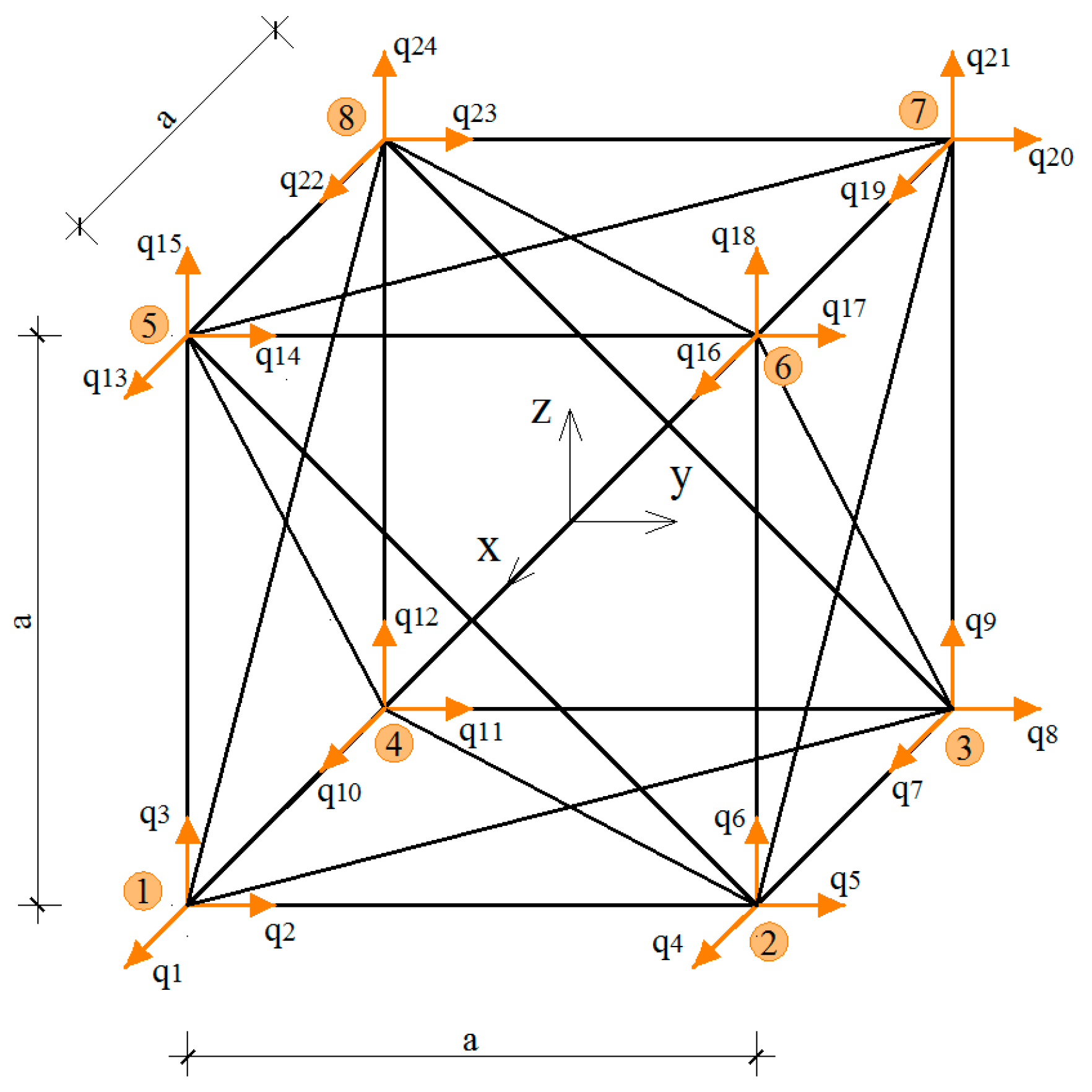
A discrete model describes a tensegrity pin-joined truss structure which is composed of
e straight and prismatic bars of the lengths
, cross sections
and Young’s modulus
. The bars are connected in nodes in which a number of
nodal displacements
and nodal forces
are defined (see [
32,
33] for details). Axial forces
can be expressed by the extensions of bars
in the form
. The extensions
are a combination of nodal displacements
,
J = 1,2,…,
s.
Bkj is a compatibility matrix of projection of nodal displacements for the directions of bar axes [
32,
33]. Additionally, the self-equilibrated system of axial forces
, which satisfy the homogeneous set of equilibrium equations
, is considered. If one considers the equations of equilibrium in the actual configuration, the moment
is acting on each bar. Angles of bar rotations
can be expressed as a combination of nodal displacements
.
Ckj is an algebraic matrix of a projection of nodal displacements for the directions perpendicular to bar axes [
34]. The above formalism leads to the linear system of algebraic equations
, in which the linear stiffness matrix
and geometric stiffness matrix
can be expressed in algebraic form
,
(see references [
33,
34] for further details). The approach is not dependent on any approximation typical for the finite element method.
In a discrete model (DM), the strain energy of a tensegrity truss can be expressed in the matrix notation as a quadratic form of nodal displacements
q:
where:
,
-global linear stiffness matrix,
-global geometric stiffness matrix.
The self-equilibrated system of axial forces of the structure is represented by the geometric stiffness matrix and is related to the equations of equilibrium in the actual configuration of the lattice.
The strain energy of a solid according to the symmetric geometrically linear 3D elasticity theory (ET) [
35] can be expressed as:
where:
-vector of strain components,
-elasticity matrix.
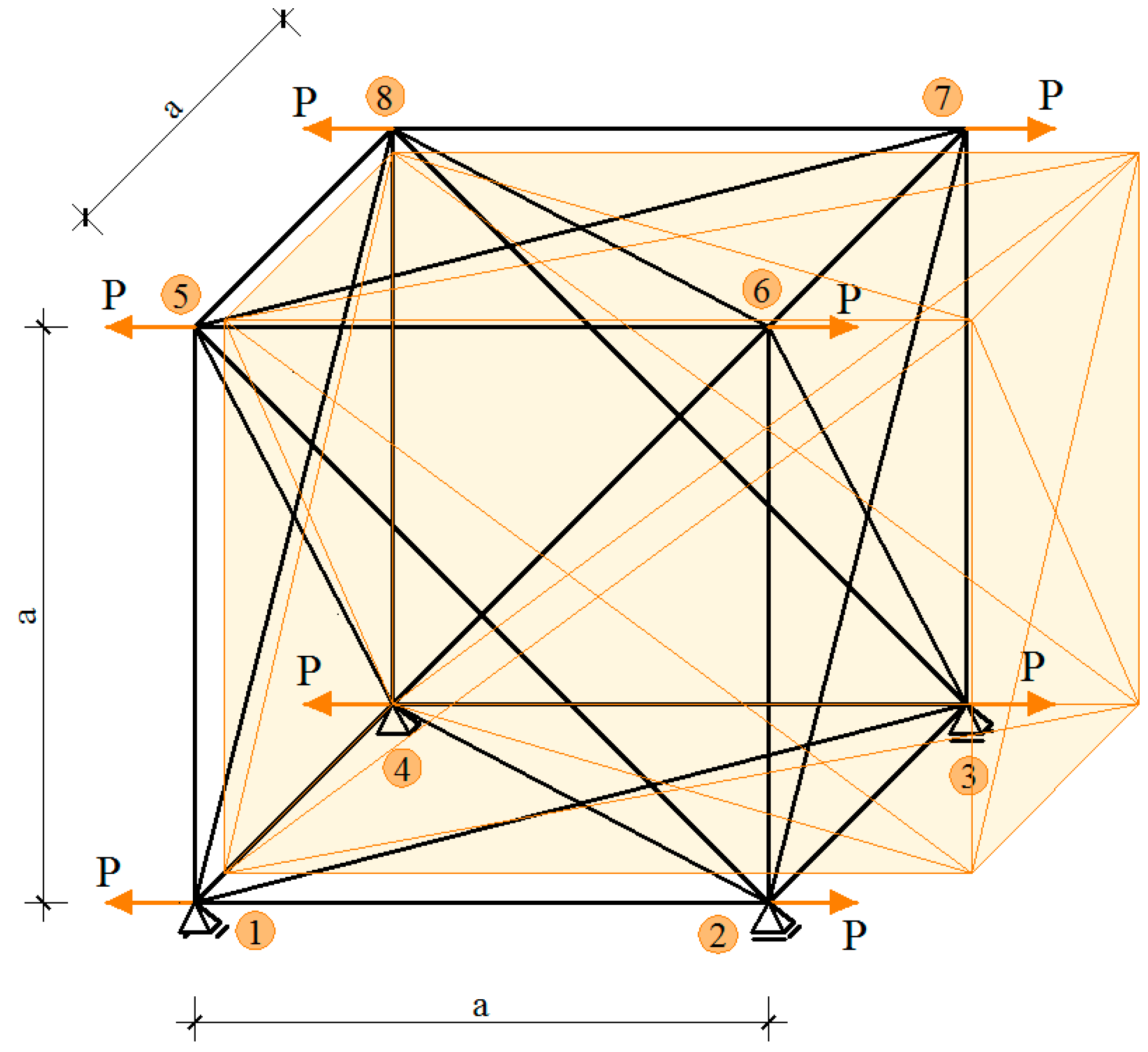
In order to analyze mechanical properties of the material, it is proposed to compare the strain energy of an unsupported tensegrity to the strain energy of a cube, with an assumption that the strain energy of the cube is constant in its volume. In a general case both the analyzed structure and the solid can have arbitrary dimensions. However, in order to show how the continuum model is constructed, a typical tensegrity module inscribed into a cube of edge length
is considered (presented in Figure 1 of reference [
28]).
With the above assumptions, the strain energy of the cube of edge length
, according to the symmetric 3D elasticity theory (ET):
To compare the energies and build the equivalent elasticity matrix, the nodal displacements of the structure are expressed by the average mid-values of displacements and their derivatives in the center of the cube of edge length , with the use of Taylor series expansion. Nodal coordinates of the analyzed tensegrity structure can be expressed using the parameter , which corresponds to the edge length of the cube: . Then, the parameters of the node i (for example nodal displacements) can be described as:, , .
The next step of the analysis is a substitution of the determined nodal displacements in the formula (1). As a result, an expression containing a constant part (independent of ) and terms with a factor , n {1, 2, …} is obtained. However, in the case of small values of , terms with the factor can be regarded as higher order terms in the Taylor series expansion and should be omitted. Small values of the module dimension should be considered as relative to the total dimensions of the metamaterial. Moreover, the mentioned terms contain displacement derivatives greater than the first one, which is beyond the scope of the symmetric theory of elasticity.
Comparison of strain energies (1) and (3) leads to the determination of coefficients of the matrix
E. In a general case of an anisotropic structure, the obtained elasticity matrix in Voight’s notation [
32] has the following form:
It contains 36 coefficients, including 21 independent ones. The above matrix can take different and particular forms, with the type depending on eight possible symmetries [
36]. The proposed continuum model is non-linear in the sense of equations of equilibrium considered in actual configuration. Numerical simulation and validation of the proposed continuum model is presented in the
Appendix at the end of the present paper. Other possible continuum models of the lattices are discussed in references [
37,
38].
3. Simplex-Based Tensegrity Lattices
The metamaterial considered in this paper is constructed from one of the most popular tensegrity modules—a 4-strut simplex (see references [
7,
9,
28] for geometrical details). It is a typical tensegrity, which consists of four separate struts surrounded by the continuous system of twelve cables [
7,
8]. The 4-strut simplex module is obtained from a regular prism by rotating one of its bases 135 degrees clockwise or counter clockwise.
One of the special characteristics of tensegrity structures are infinitesimal mechanisms that are balanced with a self-equilibrated system of normal forces [
7,
8,
10]. The considered simplex module has one infinitesimal mechanism and one corresponding self-stress state—self-stress is expressed by the relative forces in struts and cables with a multiplier S
0 (see reference [
28] for the detailed description).
It should be noticed that the proposed unit cell is an anisotropic structure. However, it is proved below that the metamaterial based on such unit cells exhibits orthotropic properties.
Simplex tensegrity modules described above can be arranged in different patterns to form a material with certain properties. Depending on the type of the module used (with the basis rotated clockwise or counter clockwise) and the way in which the modules are connected, a material with different mechanical characteristics can be obtained. In the present paper a material with orthotropic properties is proposed, as it exhibits some special features (negative Poisson’s ratio as an example [
28]).
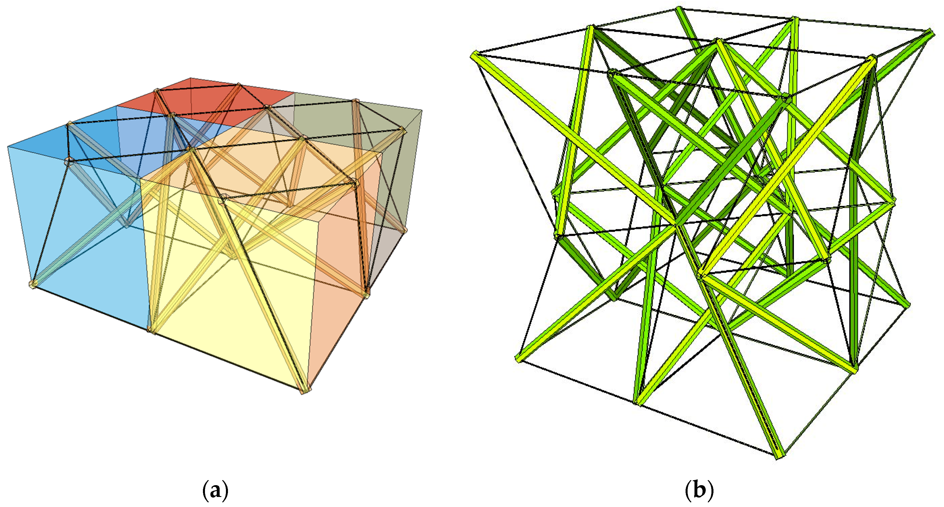
A system that consists of four simplex modules joined together by common cables of the lower bases and common nodes of the upper bases is presented in
Figure 1a. The modules are arranged alternately: a module that is rotated clockwise is put next to the module with the counter-clockwise rotation. Although a single simplex module is anisotropic, the whole structure has orthotropic properties. Following this method, a regular eight-module supercell (
Figure 1b [
28]), constructed using two four-module layers, was considered. The upper layer of the supercell was built from the four-module layer turned upside-down and connected with the bottom layer using common cables.
The elasticity matrix
obtained from the continuum model of the considered regular supercell has the following form:
with the coefficients [
28]:
where:
,
,
.
The volume of the regular lattice is .
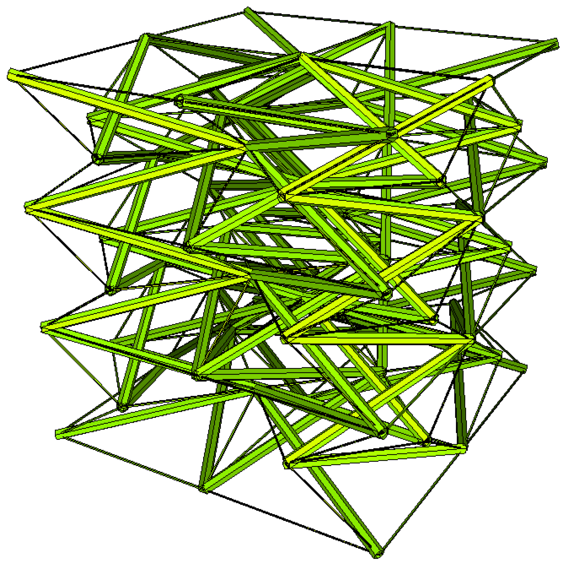
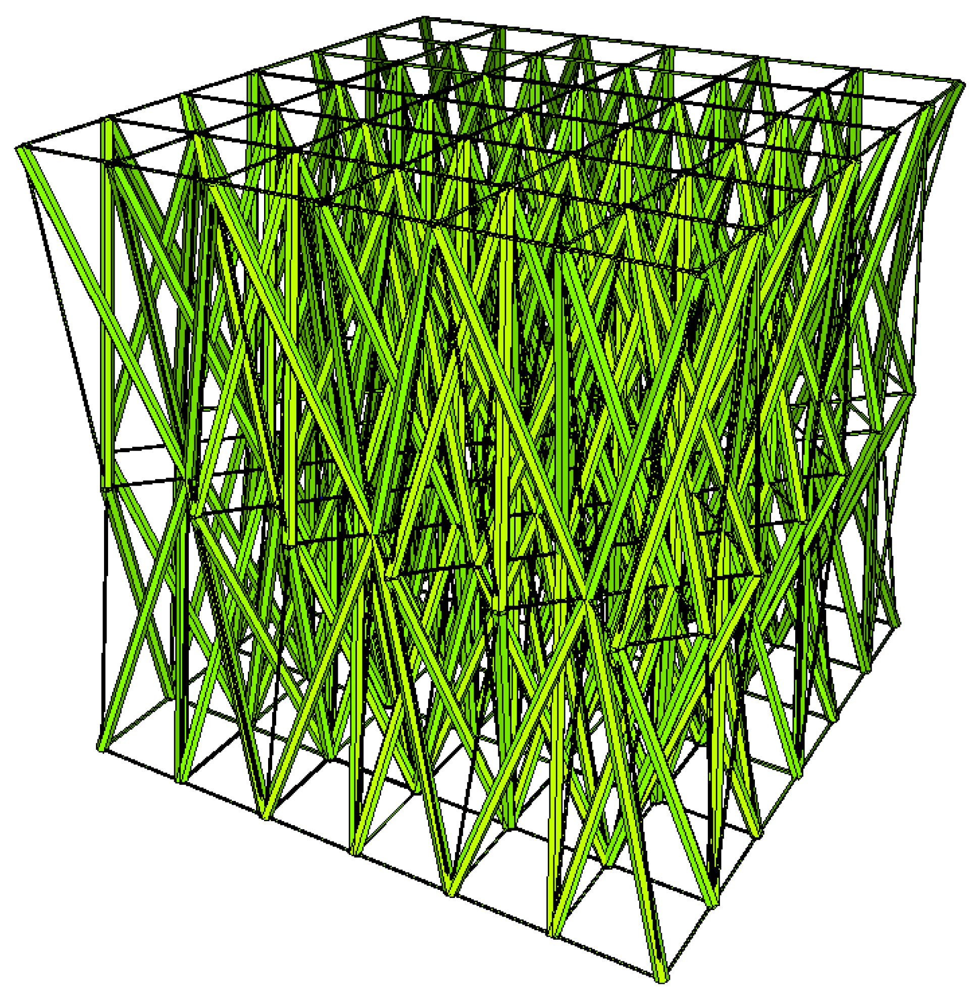
Two other tensegrity lattices inscribed into a cube
are considered: with a small and large height-to-base area ratio of the module (
Figure 2 and
Figure 3).
Self-equilibrated forces for (L) and (H) models differ from the ones presented in
Figure 1. The elasticity matrices
and
have orthotropic structures as before, but with different coefficients:
with the volume
and
with the volume
.
The supercells are representative because the mechanical properties described in elasticity matrices do not change in repetitive bigger volumes.
The proposed tensegrity metameterials (L), (R) and (H) will be compared and analyzed in the next chapter according to the eigenvalues and eigenvectors of the elasticity matrices under the assumption of an equal total volume.
4. Extreme Properties of Tensegrity Lattices
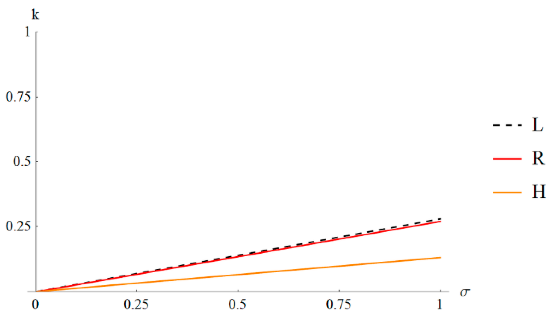
The eigenvalues (i = 1, 2, …, 6), and orthogonal eigenvectors of elasticity matrices of the proposed metamaterials depend on the parameters and . The eigenvalues in this chapter are calculated for the (L) and (H) elasticity matrices calibrated to an even volume of the material in each lattice (as in the metamaterial (R)).
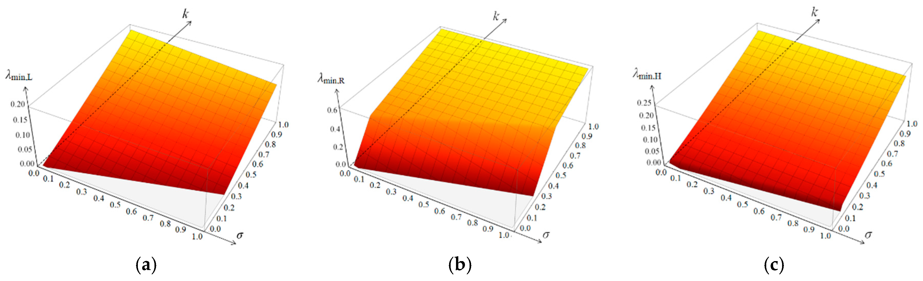
Let us start the analysis from the lowest eigenvalues. The elasticity matrices are positive definite so only positive eigenvalues are to be considered. The values of
for
and
for low (L), regular (R) and high (H) metamaterials are presented in
Figure 4.
In the (L) metamaterial (
Figure 4a) the lowest eigenvalue does not change the mode of deformation within the considered area. The metamaterial is unimode according to the classification of reference [
29]. In the (R) metamaterial (
Figure 4b) the change of the mode of deformation of the lowest eigenvalue is observed but far from the zero line. The material is also unimode for selected parameters. In the (H) metamaterial (
Figure 4c) the change of the mode of deformation of the lowest eigenvalue is observed close to the zero line. It means that the material is close to bimode [
29]. The lines of zero values representative for unimode soft deformation are presented in
Figure 5 for all metamaterials together.
The highest eigenvalues of the matrices E depend on the parameters and to a small extent (a couple of percent), therefore the analysis is not considered in this paper.
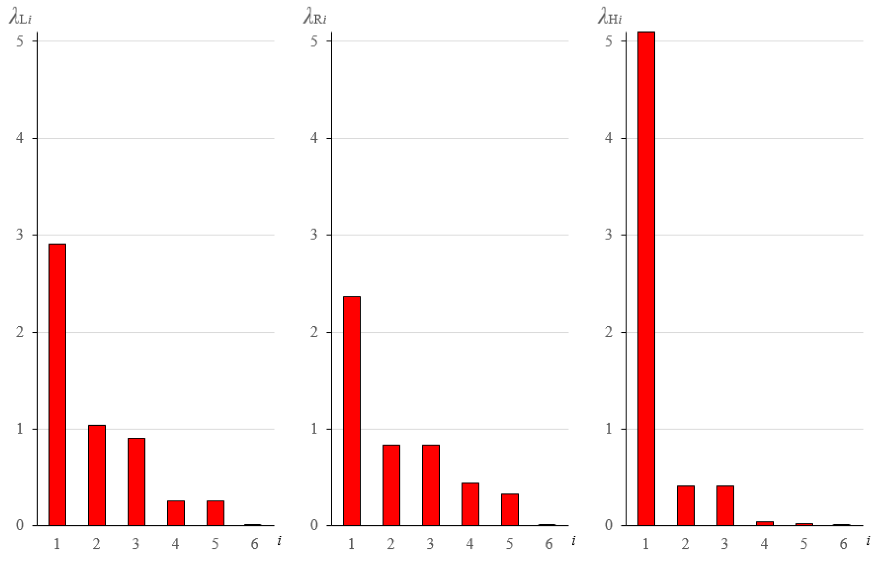
The second part of the analysis is proposed for the parameter
which is typical for standard cable-strut structures. The values of self-stress parameters necessary to obtain the zero lowest eigenvalue are then the following:
,
and
. The sets of six eigenvalues are presented in
Figure 6.
As it can be noticed, the most extreme metamaterial is (H). One eigenvalue is high, three are relatively small and two are close to zero. The (H) metamaterial is nearly bimode. The materials (L) and (R) can be defined as unimode. The sequence of eigenvectors in the (L) metamaterial is different than in the others—the double eigenvalue which is responsible for shear vertical deformation is next to the zero eigenvalue in the material (L) and next to the highest eigenvalue in the materials (R) and (H). Six deformation modes can be defined in the metamaterials: stiff (extensional), soft (extensional), named “easy” in [
29], medium extensional, high shear (double) and low shear. The results are presented graphically in
Table 1,
Table 2,
Table 3,
Table 4 and
Table 5.
The analysis carried out above for the parameter differs for other values. A similar analysis can be performed on the basis of the matrix inverse to E, defining others that can be called stress modes instead of deformation modes.
5. Conclusions
The present paper focuses on the analysis of a novel cellular metamaterial based on the simplex tensegrity pattern recognized as a metamaterial. Three tensegrity lattices are proposed, which differ in geometrical proportions. The authors use a continuum model of the lattices to estimate the influence of self-equilibrated normal forces and geometrical parameters on the behavior of the system. Moreover, a spectral analysis of the elasticity matrices, with the condition of the equal total volume of the lattices, is presented as a tool for comparing the metamaterials and defining their extreme properties.
The performed analyses allowed the authors to identify six typical deformation modes in the lattices, which were named stiff, soft and medium extensional modes, as well as high (double) and low shear modes. The proposed novel simplex based metamaterials can be regarded as extreme materials with unimode or nearly bimode mechanical properties. The occurrence of soft (easy) as well as stiff deformation modes allows for classifying the developed materials as smart tensegrity metamaterials, which is very promising as far as the engineering applications are concerned.


