1. Introduction
Today, the investigation of engineering problems involving the use of large deformation materials such as silicon, rubber, or biological materials has focused the attention of many researchers [
1]. One typical field of research for such materials is the analysis of their contact behaviour during indentation experiments. These materials exhibit large displacements under contact loading due to their physical behaviour. One major difficulty in the analysis of contact problems in hyperplastic materials is that their mechanical behaviour cannot always be described by theoretical models [
2]. Some analytical [
3,
4,
5,
6,
7,
8,
9] and numerical [
10,
11,
12] studies can be found in the literature that have contributed to a better knowledge of such a problem, but they often consider different assumption for their analysis, such as assuming small strains below the elastic limit [
6,
8,
11], considering half-plane elastic for both the indenter and the soft body material [
7,
9,
11,
12], assuming that the contact area is much smaller than the radius of the indenter and the elements are frictionless [
7,
10,
11], or that the external angle of the indenter is very small [
8]. Nevertheless, some of these assumptions are not always well supported by lab experiments. Although experimental techniques constitutes an important alternative to validate analytical models and numerical studies, no substantial work can be found in the literature [
2,
13,
14,
15,
16] for the analysis of large deformation materials.
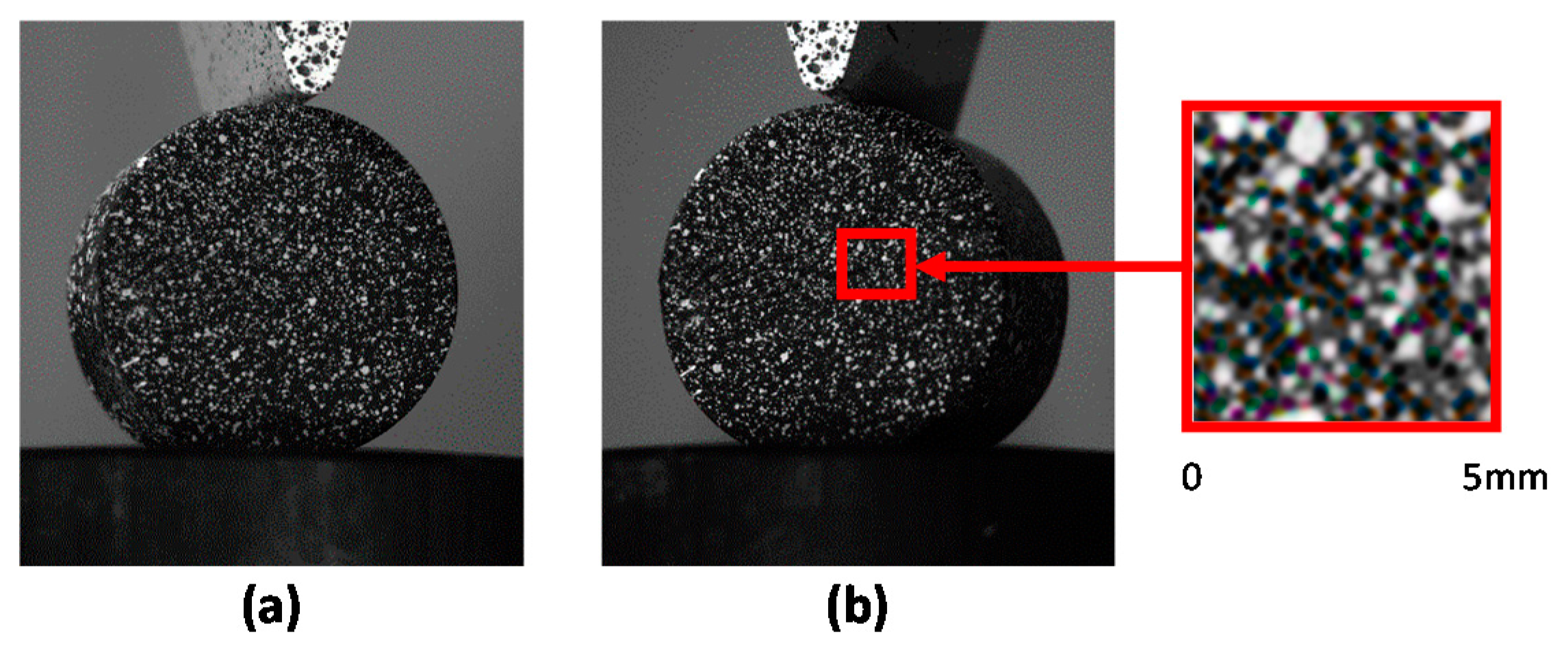
In this paper, one of the best established optical techniques for full field displacement measurement is applied to the analysis of large strains due to indentation in a hyperplastic material. The adopted technique is 3D digital image correlation (3D-DIC) [
17], which employs at least two cameras for a stereoscopic visualization of the surface of the specimen with a random distribution of light intensity (speckle). The element surface can be unambiguously distinguished by its random neighbourhood pattern. In this way, a group of pixels corresponding to a specific location at the element surface is identified on a sequence of images captured during deformation with the aid of an image correlation algorithm [
17]. Displacement fields of the studied surface are obtained, and from them, strain maps can be also calculated.
3D-DIC is employed for the analysis of contact experiments using a wedge-shape indenter on a soft material cylinder. The experiment was performed to obtain displacements and strains fields. Two analytical studies employing Finite Element Method representing the experimentation were also performed. Those analyses employed two different mathematical formulation to determine the material behaviour.
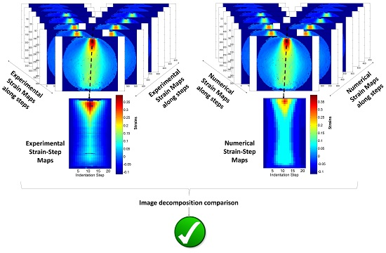
During the experiments, it was not possible to guarantee avoiding solid rigid displacement, which could affect to the displacement measurements with 3D-DIC. For that purpose, it is believed that strain maps more adequately represent the mechanical behaviour of the material during the test rather than displacement maps. In order to evaluate the accuracy of the numerical simulation performed using FEM models, strain maps from the experiments and FEM were compared. The compassion of strain maps obtained by employing different methodologies is a challenging task. In this paper, a novel methodology based on the decomposition of the strain maps from both experiment and simulation was evaluated to perform quantitative comparisons of the indentation process at different displacement steps. The adopted comparison methodology is based on an Image Decomposition algorithm [
18]. It consists of the decomposition of each data field into a feature vector that is independent from scale or orientation of the original data map. It is necessary to decompose each of the displacement maps captured along the test in order to study an event through time. Nevertheless, this paper presents a novel procedure to encode the full experimentation in a single strain map (based on Tchebichef shape descriptors [
19]). This procedure decreases the dimensionality of the comparison process compared to some previous work [
2,
20].
3. Results
The experimental and numerical results of the indentation performed on the rubber cylinder are presented here together with the results of the comparative employing image decomposition. As mentioned above, the large amount of displacement and strain maps makes it necessary to reduce the presented data in order to accelerate the their direct comparison.
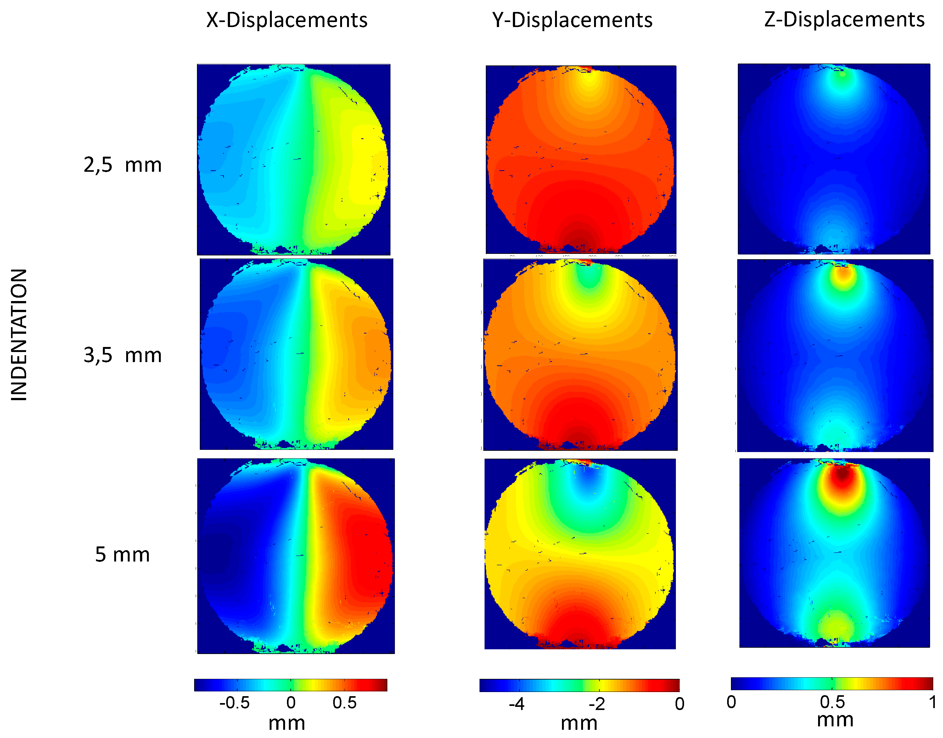
For illustration purposes,
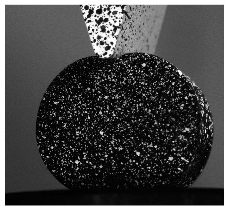
Figure 7 shows the displacement maps obtained at three different indentation steps (i.e., 2.5, 3.5, and 5 mm) in the three spatial directions. As observed, there are some areas where the results were not successfully monitored due to the large level of deformation achieved. That is especially notorious in the upper area, where the contact with the indenter occurred, and in the lower area, where the specimen was supported.
In addition, some tilting on the displacement maps was also observed. This orientation was due to the angles required in the stereoscopic camera system to perform 3D-DIC. Nonetheless, the orientation of the axis coordinate system was selected to have a Y-axis in the direction of the indention and a perpendicular X-direction in order to have the same coordinates systems for both the experimental and FEM results.
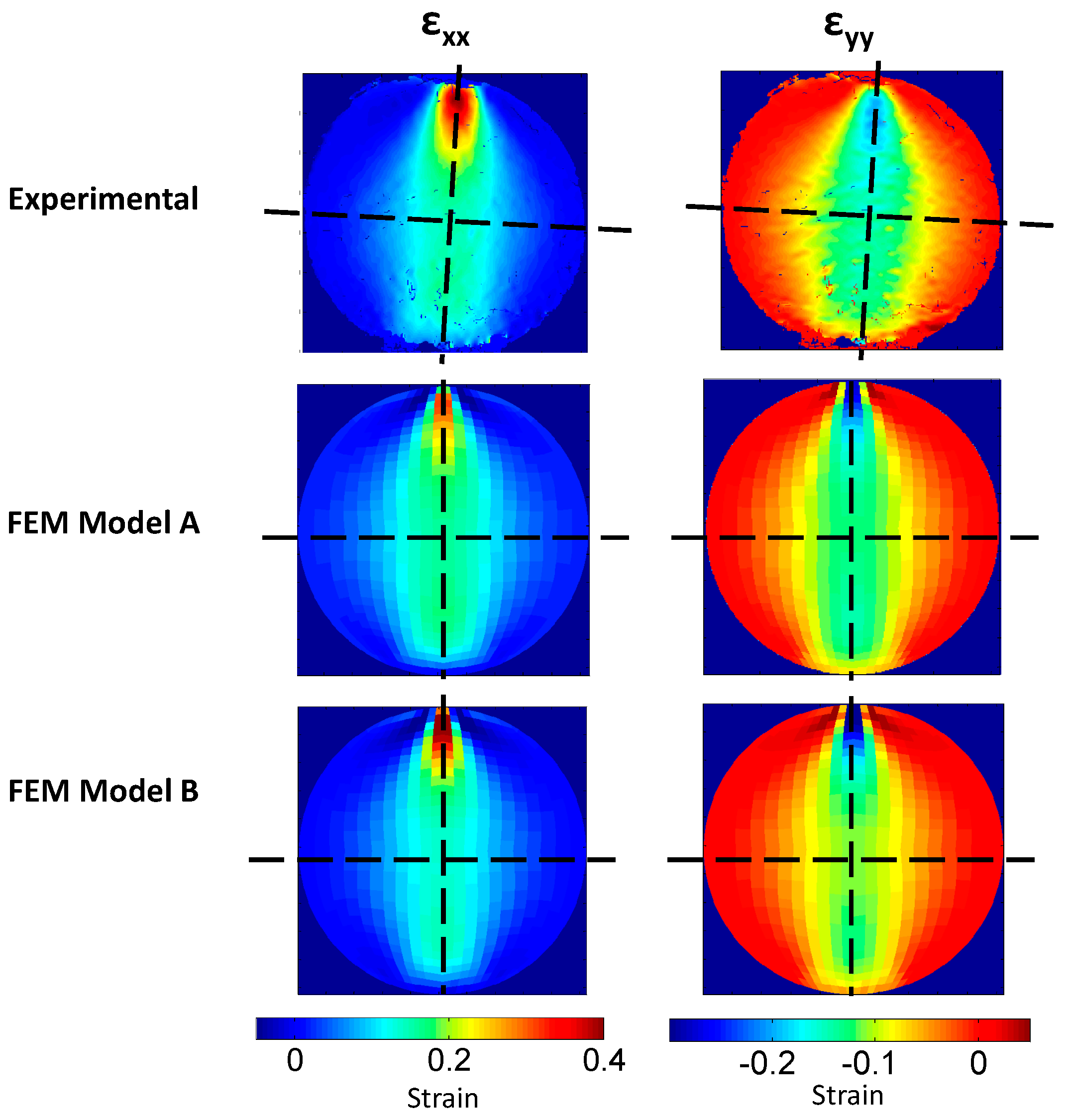
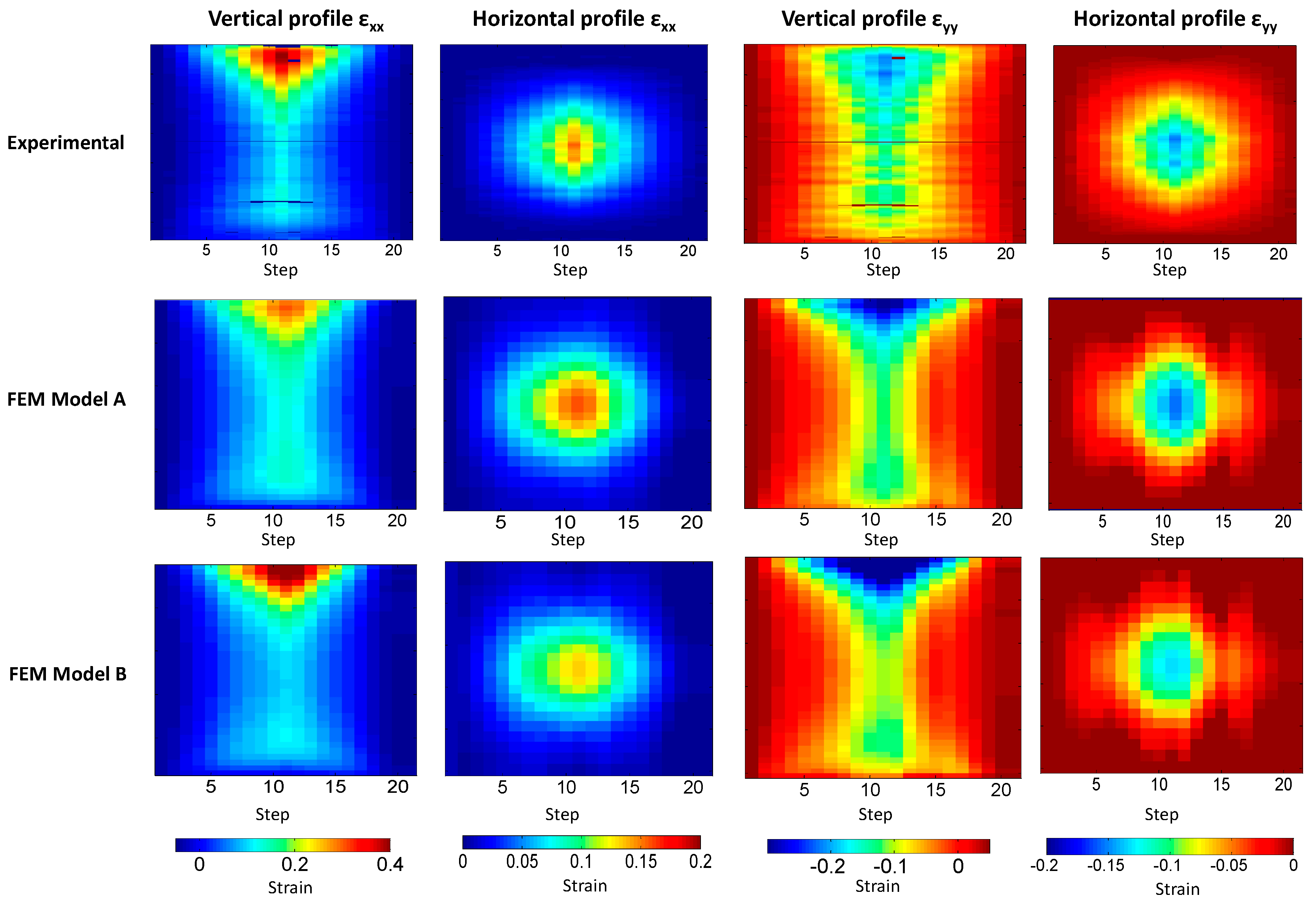
As previously mentioned, the focus was placed on the strain fields instead of the displacement fields to avoid possible solid rigid displacements and to analyze the material mechanical behavior. Hence,
Figure 8 presents the experimental and numerical strain maps in X and Y directions (ε
xx and ε
yy respectively) obtained at maximum indentation of 5 mm on the rubber specimen.
As observed, strain maps obtained with FEM are very close to those obtained during the experiments. However, it is observed that no direct quantitative full-field comparison is possible due to the differences in size of the strain map and the orientation of the experimental strain maps.
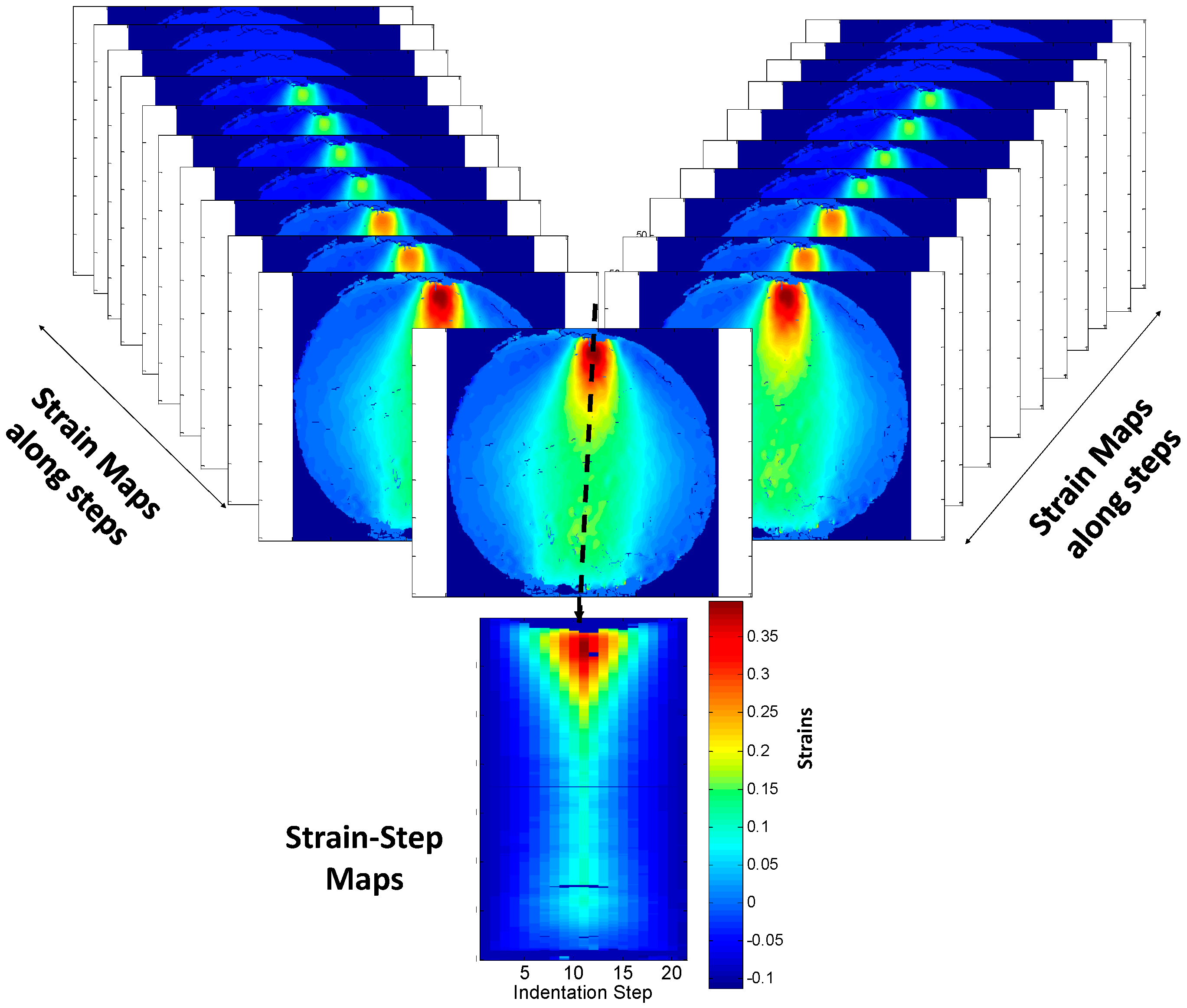
To overcome these drawbacks, the vertical and horizontal profiles are presented in
Figure 8 as black dashed lines. The data of 126 strain maps considered in this study are simplified into 12 data fields encoding the strain data (strains-step maps) along the 21 steps, as presented in
Figure 9.
A good correlation between experimental and numerical results is observed in
Figure 9. However, some slight differences are present, and some quantification of them is required to define which numerical model represents the experimentation more adequately.
Feature vectors make it possible to quantify differences by calculating the Euclidean distance between them. The Euclidean distance is simply the straight-line distance between the locations represented by the vectors in a multi-dimensional space, so that two coincident vectors have a Euclidean distance of zero.
Table 1 shows the differences obtained between the strain-step maps presented in
Figure 9.
The differences are in a lower order of magnitude of one tenth of the maximum strain value. Since feature vectors have the same length, a correlation coefficient between experimental and both numerical results was also calculated. This concordance correlation coefficient provides an indication of the extent to which the components of the feature vector fall on a straight line of gradient unity when plotted against one another. The concordance coefficients for the shape descriptors are presented in
Table 2 as a percentage in order to represent the similitude of the strain-step fields.
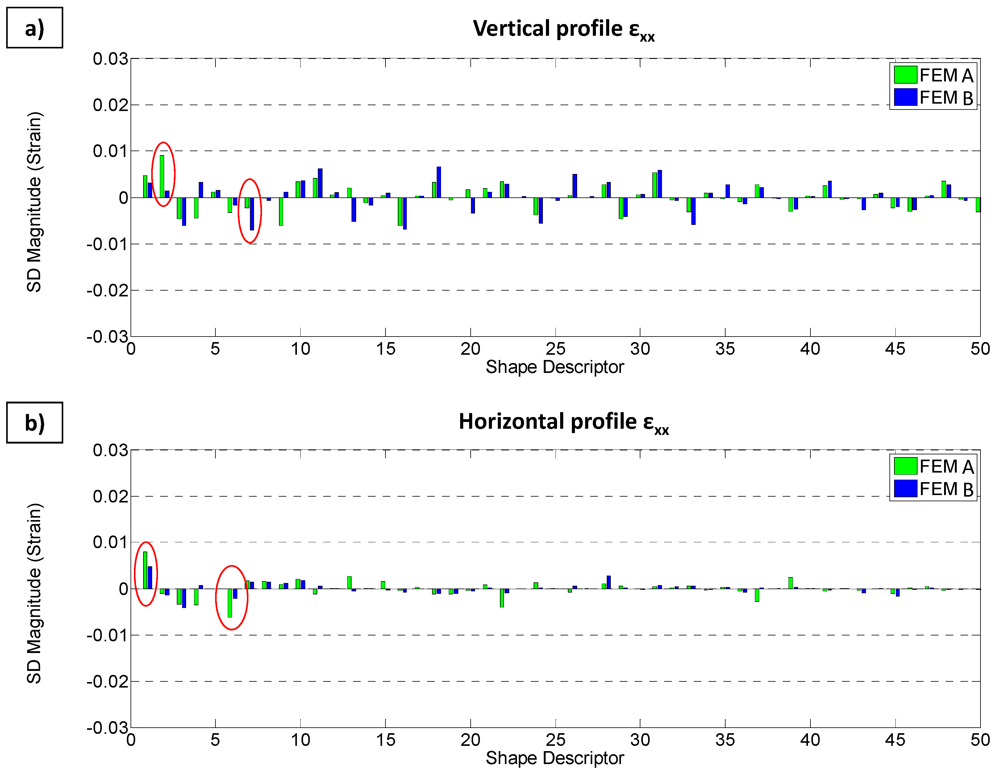
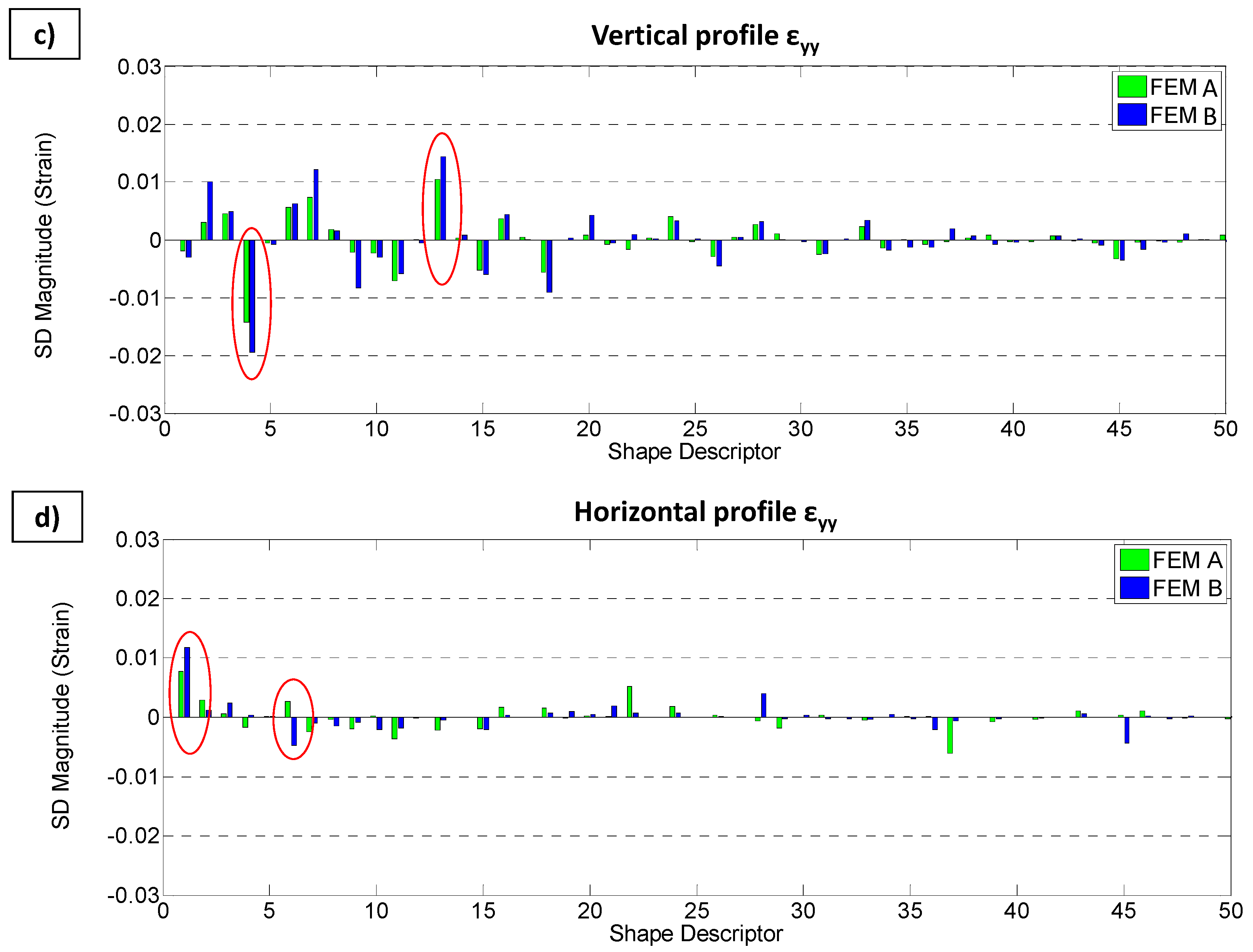
Finally, it is interesting to plot the residuals of the differences between feature vectors in order to observe if any of the shape descriptors show larger differences, which could give information about the evolution of the differences along the studied steps.
Figure 10 presents bar graphics of the residuals corresponding to the four strain-step maps (i.e., the vertical and horizontal profiles for ε
xx and ε
yy strains). The residuals are calculated by directly subtracting experimental and FEM feature vectors. The focus is placed on the two shape descriptors that offer maximum differences (red circles in
Figure 10).
It is clearly observed that differences in the shape descriptors values are very small.
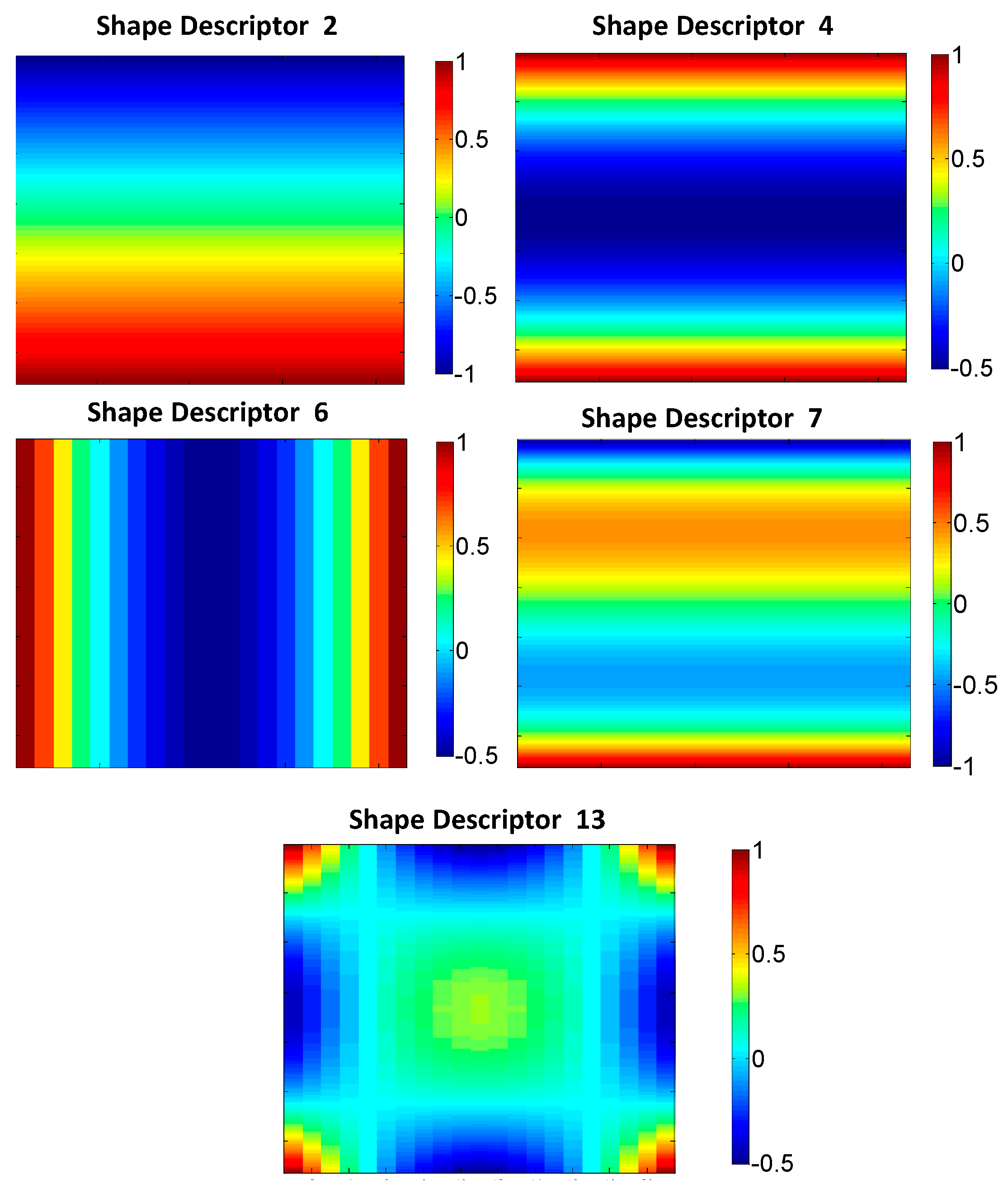
Figure 11 shows the kernels of the Tchebichef shape descriptors with higher differences. These kernels illustrate the distribution of the normalized residuals along the strain-step map in a two-dimensional representation. Thus, they also provide information about the evolution of the differences along the indentation.
Bigger differences in ε
xx and ε
yy strain-step maps for horizontal profiles are observed in SD#1 and #6. In the case of ε
xx strain-step maps for the vertical profile, larger differences are observed in SD#2 and #7. Finally, in the case of ε
yy strain-step maps for vertical profile, larger differences are observed for SD#4 and #13. The kernels of those shape descriptors are presented in
Figure 11. However, the kernel of SD#1 has a homogenous value indicating a full field offset in the strain value along the 21 studied steps, and it has not been considered in
Figure 11.
4. Discussion
It is important to emphasize that the reduce area of interest and the high deformation level achieved during deformation made the calculation of the displacements maps using DIC complex. Additionally, as observed in
Figure 7 and
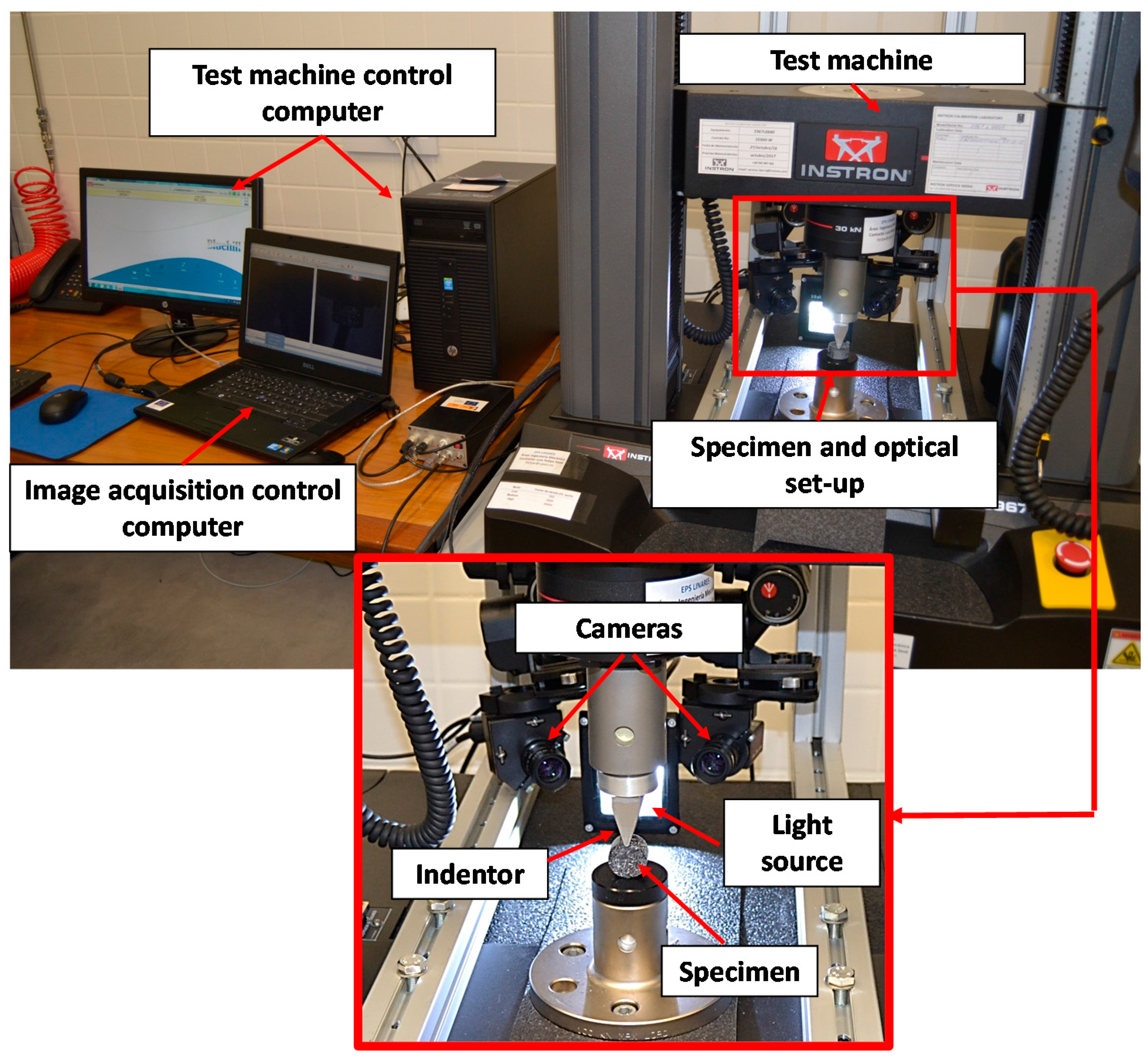
Figure 8, the indenter and the support of the specimen created some shadows and blind areas that made the visualization of some areas at the instant of maximum indentation difficult. To maximize the visualization of the whole area of interest during the full indentation and release, a specific optic set-up was required, as observed in
Figure 2. With this optical arrangement, an uncertainty in the measurement of 31.7 µε was achieved when considering the similar set up employed by Tan et al. [
2].
Displacement maps obtained by this experimental procedure is presented in
Figure 7. As observed, some negligible non-correlated areas are present (dark spots). It particular, some regions close to the indenter and at the lower area of the specimen were not able to be processed due to the high distortion, shadows, and the obstruction of the indenter in the cameras view, as shown in
Figure 12.
Those non-data areas are also present in experimental strain maps shown in the first row in
Figure 8, where strains at maximum indentation are presented. Moreover, no large differences are observed by comparing those experimental and numerical results from Finite Element model A (and from Finite Element model B). However, it is observed that the FEM A model shows slightly lower maximum values in ε
xx (0.32 ε) and lower minimum values in ε
yy (0.30 ε), while the FEM B model presents slightly higher values in ε
xx (0.44 ε) and ε
yy (0.34 ε ) compare to experimental ε
xx and ε
yy values (0.39 and −0.25 strain, respectively).
Moreover, the focus is placed not only in point differences but in performing a full field comparison along the complete experiment. For this purpose, the strain-step images presented in
Figure 9 show how the vertical and horizontal profiles of ε
xx and ε
yy varied along the studied step. Moreover, the creation of these strain-step maps allowed image decomposition to be performed through Tchebichef formulation, which is not applicable in non-rectangular data fields [
19]. Moreover, it is observed that these strain-step maps agree between them. To quantify these differences, strain-step maps were decomposed into 50 feature vectors composed (
Table 1). FEM model A obtained lower differences that model 2 in all the strain step maps, except for ε
xx in the horizontal profile strain map. Larger differences are observed for the ε
yy vertical profile strain map for the FEM B model, which represents a difference of 14.2% respect the maximum ε
yy experimental value compare to the 10% of difference obtained employing the FEM A model.
The correlation coefficients obtained in
Table 2 show a value close to 100%, but again the results from FEM model A show higher concordance with experimental results.
An interesting analysis can be also performed observing the differences in the kernels of the SD as illustrated in
Figure 10 and
Figure 11.
Looking at the differences in ε
xx (
Figure 10a), there are more important differences in SD#2 and SD#7 between experimental results and those obtained by the FEM A and FEM B models, respectively. From the representation of kernel of SD#2 in
Figure 11, it is observed that the value of experimental strain in the upper area of the strain-step map is slightly bigger than the value of the FEM A model along all the steps of the indentation and, on the contrary, the value of experimental strain in the lower area of the strain-step map is slightly lower than the value of that FEM model. On the other hand, from the representation of kernel of SD#7, it is observed that differences between experimental and FEM B models are also present along the horizontal axis, which means that they are present along all indentation steps. It is also observed that in the upper area close to the edge of the strain-step map, the experimental value is bigger that the simulated value, while in the lower area of the image, the opposite occurs. This indicates that experimental deformation is slightly more focused in the contact area compare to the numerical results. Moreover, the FEM B simulation values are bigger than experimental results just above the half of the strain-step map and are lower just under it.
Differences in ε
xx (
Figure 10b) suggest that the larger differences between FEM A and experimental results are associated on SD#1 and SD#6. As previously mentioned, SD#1 refers to a full field offset. In this case, the general experimental value of ε
xx horizontal profile is lower than the value of FEM A. Additionally, from the kernel of SD#6 in
Figure 11, it is observed that an evolution of the difference exists, reaching it maximum values at the central area of the map, which implies the maximum indentation instant. That difference indicates that the values of experimental ε
xx are lower than FEM A results mainly at that instant.
With respect to the differences in ε
yy (
Figure 10c), the differences between shape descriptors are slightly bigger than in the rest of the cases, as illustrated in
Figure 10. These differences are more focused in SD#4 and #13 and between the experimental and FEM B results. Attending to the kernels of SD#4, a discordance along the whole indentation is observed where the vertical edges of the vertical profiles are bigger in the FEM B model rather than in the experimental results. Additionally, the values of experimental data in the central area are bigger than those of FEM model B.
Finally, bigger differences between both FEM models and experimental data are focused in SD#1, which means that both FEM models predicted a slightly bigger value in ε
yy along the horizontal profile than that which was measured experimentally (
Figure 10d). However, this difference is larger for FEM B. SD#13 also presents some discrepancy to the central area of the strain-step map. This discrepancy is different for FEM A and FEM B models. In the case of FEM A, ε
yy was slightly larger than the experimental results, and the opposite happened for FEM B.
5. Conclusions
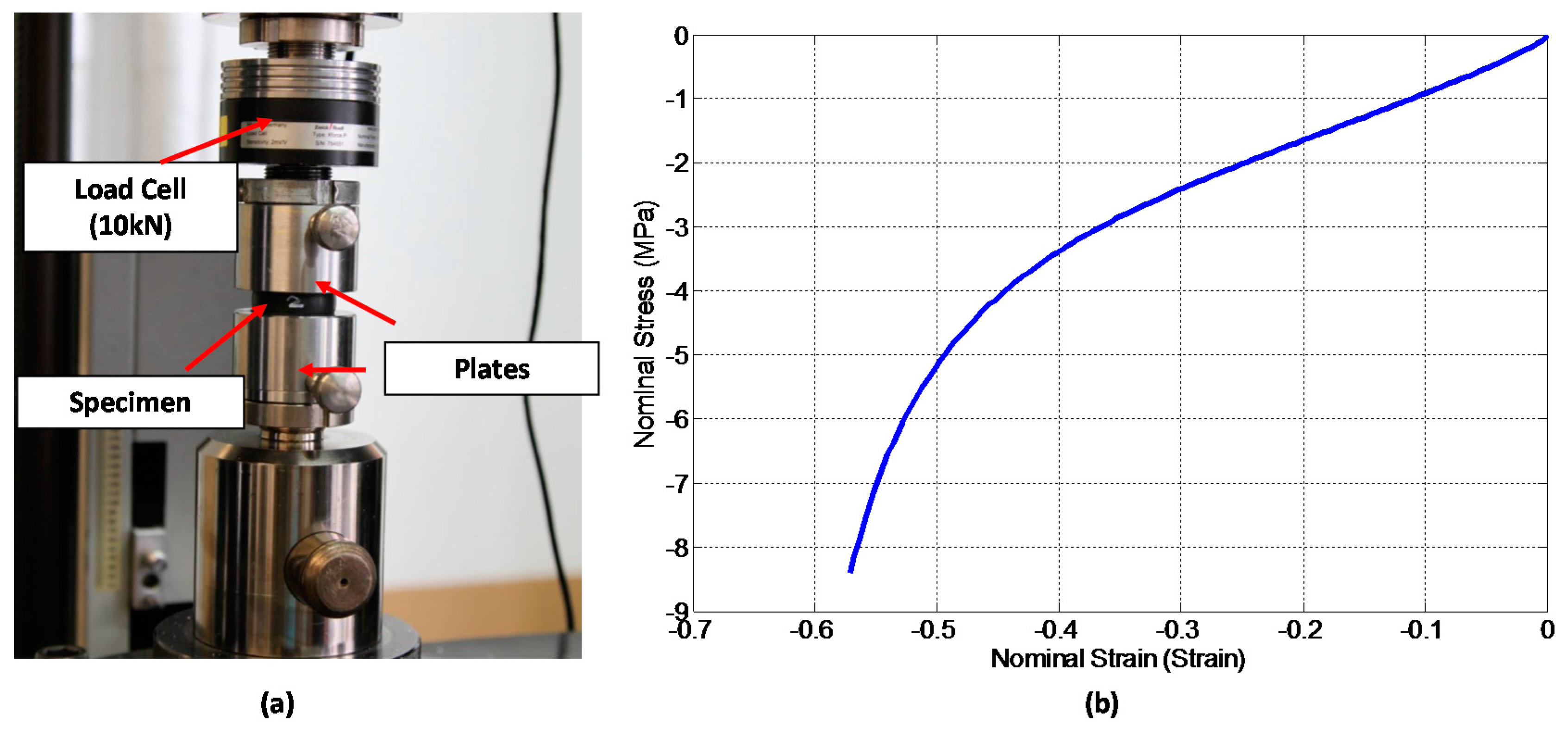
This paper presents a procedure to validate finite element models of indentations in soft materials. The validation was demonstrated by performing an experiment where a rubber cylinder (25 mm diameter and 15 mm high) was subjected to a lateral quasistatic indentation and subsequently released by a rounded edged rigid indenter. Three-Dimensional Digital Image Correlation was employed to calculate three-dimensional displacement fields from which strain maps were calculated. Two finite element models were developed to simulate the experimentation according to two different material models, i.e., Neo Hooken (FEM A) and Van der Walls (FEM B). The validation of those models was performed by comparing strain fields along the complete indentation process by employing image decomposition.
The adopted validation procedure is based on a quantitative comparison of the strain fields in X and Y directions. εxx and εyy strain maps for each of the studied steps (21 εxx strain map and 21 εyy strain map for each model and experimentation procedure) were combined into two strain-step maps for each procedure. Those strain-step maps where quantitatively compared by employing an Image Decomposition method based on Tchebichef shape descriptors. This methodology quantified differences between experimental results and models that were lower than 10% in case of FEM A. Correlation values between experimental and predicted values were always above 93%, and in the case of FEM A, the correlation factor achieved 97.1%. In addition, differences between strain fields were evaluated along the evolution of the indentation through the study of the kernels of the Shape Descriptors, which offered more important differences.
The validation procedure concluded that the FEM A model (Neo Hookean) better predicts the experimental data than the FEM B model (Van der Walls), which agrees with previous estimations [
26].
The quantitative validation approach to comparing strain fields presented herein could provide an intervention methodology to easily validate dynamic (even at high speed) indentation models, enormously reducing the data sets. Additionally it is suitable in cases where the specimen studied is not rectangular, avoiding certain restrictions of some Image Decomposition procedures.

 ,
, 


