A Novel Dynamic Co-Simulation Analysis for Overall Closed Loop Operation Control of a Large Wind Turbine

Abstract

A novel dynamic co-simulation methodology of overall wind turbine systems is presented. This methodology combines aerodynamics, mechanism dynamics, control system dynamics, and subsystems dynamics. Aerodynamics and turbine properties were modeled in FAST (Fatigue, Aerodynamic, Structures, and Turbulence), and ADAMS (Automatic Dynamic Analysis of Mechanical Systems) performed the mechanism dynamics; control system dynamics and subsystem dynamics such as generator, pitch control system, and yaw control system were modeled and built in MATLAB/SIMULINK. Thus, this comprehensive integration of methodology expands both the flexibility and controllability of wind turbines. The dynamic variations of blades, rotor dynamic response, and tower vibration can be performed under different inputs of wind profile, and the control strategies can be verified in the different closed loop simulation. Besides, the dynamic simulation results are compared with the measuring results of SCADA (Supervisory Control and Data Acquisition) of a 2 MW wind turbine for ensuring the novel dynamic co-simulation methodology.

1. Introduction

The growth of global population and the shortage of fossil fuel energy have enhanced the need for alternative energy. Of all the renewable energies, wind energy is recognized as one of the most important renewable energies due to the large power capacity and the expansion of wind farms [1]. Furthermore, the number of wind power plant installations has risen gradually worldwide after the offshore wind farm was developed. Due to the different locations of wind farms, such as onshore and offshore, the requirements for wind turbines change depending on the category of the wind and its location. In order to analyze the efficiency and reliability of the chosen wind turbine, it is important for users to predict the response before installing it. Thus, a trustworthy simulation software is required to test the wind turbine in certain wind farms. For simulation packages used for power system studies, such as the Power System Simulator for Engineering (PSS/E), reasonably accurate and low-capacity-demanding models using all system components are usually required [2]. However, the comprehensive knowledge requirement of the wind turbine makes simulation more difficult to integrate. Computational fluid dynamics and multibody dynamics should be calculated simultaneously under one interface. Furthermore, the diversity of wind turbine design and user-based controller strategies should be taken into consideration. Therefore, it is necessary to simplify the model to a certain level which is acceptable for grid simulation programs and building up a co-simulation interface [3].

Wind turbines convert the wind energy into mechanical energy and then transform it into electric energy. In general, there are two kinds of wind turbines driven by different aerodynamic forces, horizontal-axis wind turbine (HAWT) [4] and vertical-axis wind turbine (VAWT) [5]. Compared with VAWT, HAWT is widely developed in large-scale wind turbines because of its better aerodynamic behavior and higher power coefficient in high tip-speed ratio.

Of all the large-scale horizontal-axis wind turbines, HAWT can further be categorized into different types owing to its working design: constant speed, variable pitch, and variable speed type. Relevant researches have been published since the late twentieth century. A simple strategy with stall control and fixed blade was developed in 1988 [6]. Freeman and Balas [7] made a system identification of the dynamic models of wind turbines with experiments. In order to simulate the turbine dynamic, several researches about modeling have been investigated: in 1991, Leithead described the roles and objective of control of wind turbine [8]. Then the model of turbine drive system was developed by Novak [9]. Subsequently, researches about the variable speed wind turbine and the correspondent subsystem control started after the 1990s. The controls of variable speed wind turbine were studied in 2000 [10]. The nonlinear control of variable speed wind turbines without wind speed measurement was discussed in [11], which also integrated both mechanical and electrical dynamics. Further researches with advanced nonlinear controller for the rated-speed and the variable-power operation regime were developed in [12].

Based on last paragraph, the dynamic simulation of wind turbines can be recognized as a key technology in the design of the wind turbine, so that the dynamic characteristics of the wind turbine can be evaluated. Several aeroelastic computational tools have been investigated and studied since 2001 [13]. For simulating the wind turbine dynamics, the simulation software FAST was released by National Renewable Energy Laboratory (NREL), and the newest version, V8.12.00a-bjj, was introduced in 2016. In 2006, Boukhezzar [14] cooperated with NREL and proposed multivariable controller for torque control and pitch control. FAST is used to build a nonlinear model of wind turbines. PID (Proportional-Integral-Derivative) and LQG (Linear-Quadratic-Gaussian) control was used and compared. Zhang [15] used FAST to simulate WindPACT-1.5MW and developed synchronized generators and multiobjectives controllers with MATLAB/SIMULINK for overall system control. In 2008, Fadaeinedjad [16] developed a Double-Feedback Induced Generator model via MATLAB and combined it with FAST. Lu [17] investigated the load computation of a 150 kW wind turbine by IEC-61400-1 via FAST/SIMULINK. In 2010, Mandic [18] proposed FAST combined with a permanent magnetic synchronous generator (PMSG) model. Furthermore, the flexibility of FAST co-simulation inspires new control strategies in power control and blade loading reduction. Besides, some novel co-simulation methodology has been developed by combining the Interface Jacobian-based Co-Simulation Algorithm (IJCSA) with computational fluid dynamics to make the simulation closer to the real physics [19,20].

However, the full system dynamic response including subsystem dynamics is still rare. The distribution of wind turbulence at different heights not only leads the unbalanced loads on the blades and tower, but also increases the difficulty of pitch control. Therefore, the dynamic response must be taken into consideration. ADAMS (Automatic Dynamic Analysis of Mechanical Systems) was first developed by MDI (Mechanical Dynamics Inc.) and then transferred to U.S. company “MSC Ltd.”, called MD Adams (Multibody Dynamics Adams) has been applied widely in many industrial design and dynamic simulations of complex mechanism and multibody systems. This software has been widely used in multibody dynamic analyses such as automobile [21], structural analysis [22], and wind turbine analysis [23].

With all the aspects shown previously, an integration of co-simulation analysis should be developed, which is also the subject of this study. This paper aims to develop the co-simulation analysis of aerodynamics, mechanism dynamics, and control system dynamics for 2 MW wind turbines. As shown in Figure 1, by combining FAST, ADAMS, and MATLAB/SIMULINK, the aerodynamic, mechanism dynamic, and control system dynamic simulation can be calculated simultaneously under different inputs of wind. Meanwhile, dynamic models of the main subsystems—such as the pitch/yaw control systems and the direct driven permeant magnetic synchronized generator (PMSG)—are developed in MATLAB/SIMULINK combined with the control strategies of the overall wind turbine system to implement power tracking control. Finally, the co-simulation results are compared with a 2 MW wind turbine for verification, and the results show that the co-simulation analysis of aerodynamics, mechanism dynamics, subsystem dynamics, and control system dynamics for 2 MW wind turbines developed in this paper can analyze the overall system characteristics satisfactorily.

2. System Model Build Up

More precisely, a turbine model, including aerodynamic forces, torque coefficient, and transmission system, was derived in FAST software. Next, the nonlinear dynamic models of wind turbine subsystem, containing one permanent magnet synchronous generator, three independent pitch control systems driven by DC motors, one yaw system driven by four AC motors, and overall system controller were built by using MATLAB/SIMULINK software. Finally, the dynamic response and multibody interaction was represented in ADAMS software.

Table 1. Specifications of software versions.

Software	Version
IEC	v5.01.01 (2010-03-18)
AeroDyn	v13.00.00a-bjj (2010-03-31)
FAST	v7.00.01a-bjj (2010-11-05)
ADAMS	v2010
SIMULINK	v7.11.0.584 (R2010b)

shows the versions of different software that were to use in this study.

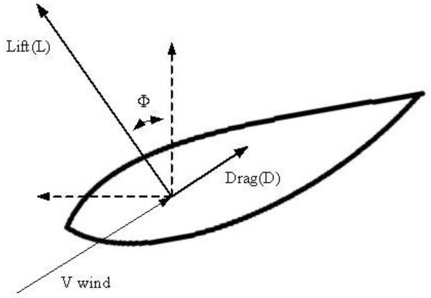
2.1. Mathematic Model of Wind Turbine System

The kinetic energy of airs through a unit area can be denoted as:

$$P_w=\frac{1}{2}\rho A{v}_w^3{C}_P(\lambda ,\beta )$$

(1)

with $P_w$ as power of the wind, $\mathsf{\rho }$ as air density, $v_w$ as velocity of the wind, and $A$ as the cross-sectional area of the blade covering region.

Based on the law of Lanchester–Betz, only some of the power can be captured by the generator. The maximum rate of power efficient is equal to $16/27\left(53\%\right)$. Normally, the power efficiency is determined by power coefficient $C_p$ which is representative of $\lambda$ and $\beta$:

$$C_p(\lambda ,\beta )=\frac{P_w}{\raisebox{1ex}{$1$}\!\left/ \!\raisebox{-1ex}{$2$}\right.A\rho v_w^3}$$

(2)

where $\lambda$ denotes tip speed ratio, and $\beta$ is blade pitch angle.

Subsequently, blade lifting force derives the turbine rotor with specific torque $T_w$, which can be expressed as Equation (3)

$$T_w=\frac{1}{2}\rho A{v}_w^{2}R{C}_q(\lambda ,\beta )$$

(3)

with blade length $\mathrm{R}$ and torque coefficient $C_q$.

Furthermore, the relation between rotor velocity and wind power can be attributed to blade element momentum theory (BEM) [21], which is combined with blade element theory and momentum theory to alleviate some of the difficulty in calculating equivalent torque on rotor drivetrain. The advantage of the BEM theory is that each blade element is modeled as a two-dimensional airfoil. Figure 2 shows the resultant aerodynamic forces on the element. These forces dictate that the thrust (perpendicular) and torque (parallel) of the rotor, which are the dominant forces for turbine design.

The aerodynamic force is applied at the center of airfoil chord line, which generates an equivalent torque. When we include two-dimensional airfoil tables of lift and drag coefficient as a function of the angle of attack, $\alpha$, a set of equations are derived that can be iteratively solved for the induced velocities and the forces on each blade element. The equivalent torque at this center equals zero so that the torque is not affected dramatically while changing $\mathsf{\alpha }$. Thus, each blade is divided into several pieces with different airfoils and lift/drag coefficients.

Figure 3 shows the relation between the lift, drag, pitching moment coefficients, and the angle of attack $\mathsf{\alpha }$ at 17,750 mm based on the blade root.

Meanwhile, the tower influence model was based on the study of Bak et al. [24]. A potential flow solution around a cylinder was used as the base flow field along with a downwind wake model dependent on tower drag coefficient $C_d$. This model also expresses the influence of the tower on the local velocity field at all points around the tower, including the raise in wind speed around the sides of the tower and the cross-stream velocity components in the tower near flow field.

Table 2. Specifications of wind turbine.

Name	Dimensions (m)	Mass (kg)
Generator	$\mathsf{\phi }3.8\times 2.2$	4900
Nacelle	$3.5\times 2.8\times 2.8$	12,000
Hub	$2.5\times 2.2\times 2.2$	19,000
Blade	34	5500
Tower	61.859	100,000

denotes the specification of blade/tower parameters with all the parameters measured from a 2 MW wind turbine.

After finishing the model mathematic setup, a geometric preference can be exported in ADAMS software with specific joints and applied aerodynamic force in Figure 4. The model is a simplified expression of components. The kinematics and dynamics are calculated in terms of Jacobian matrix and Eulerian representation.

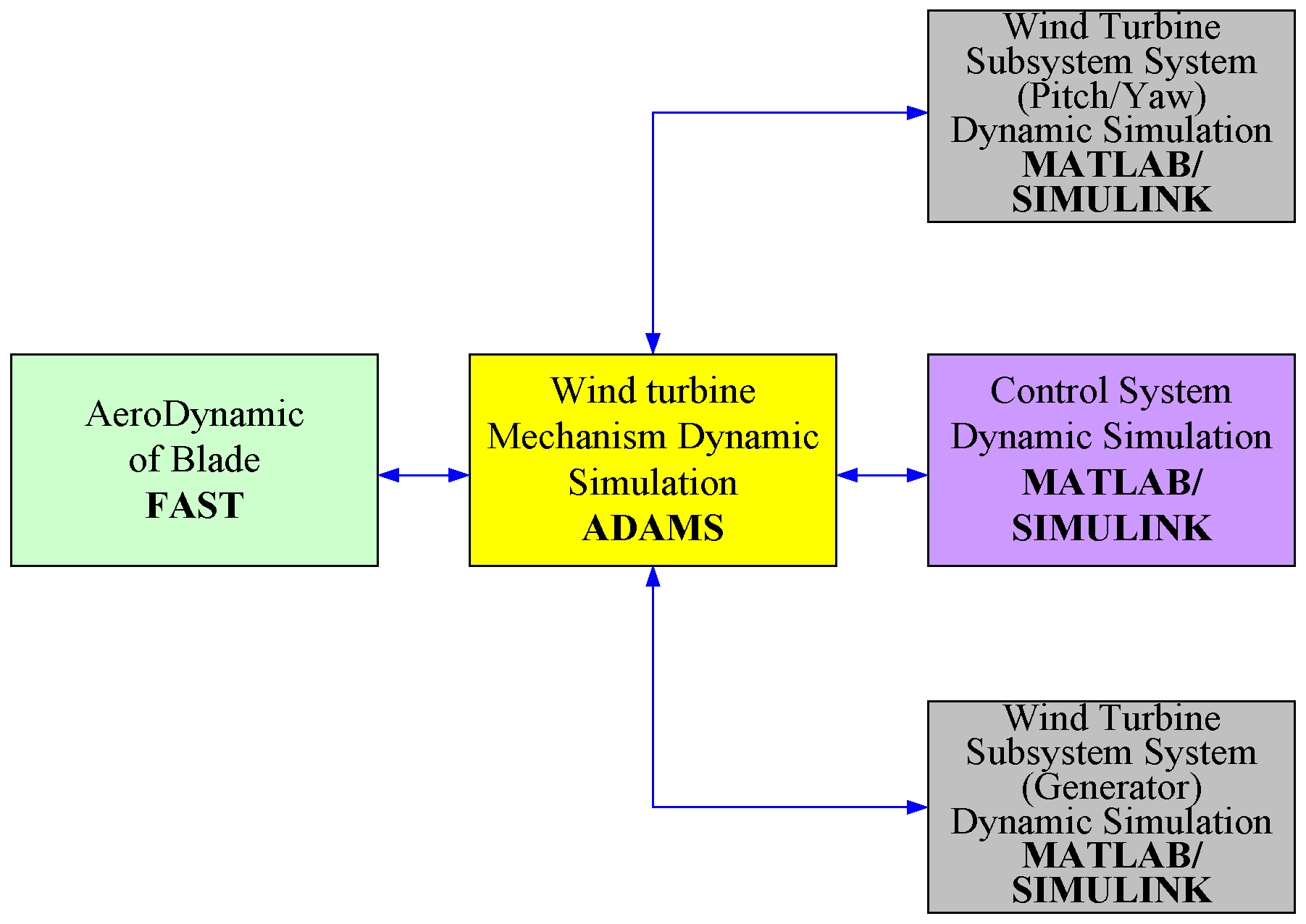
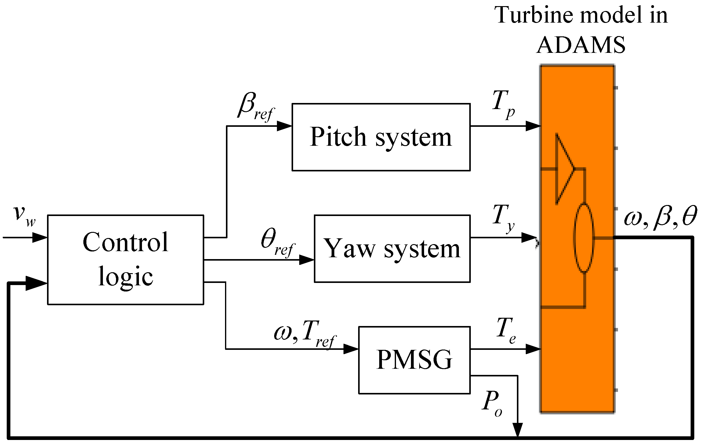
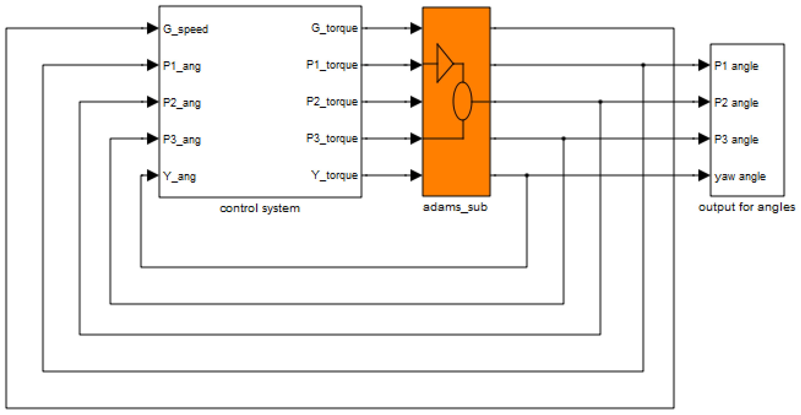
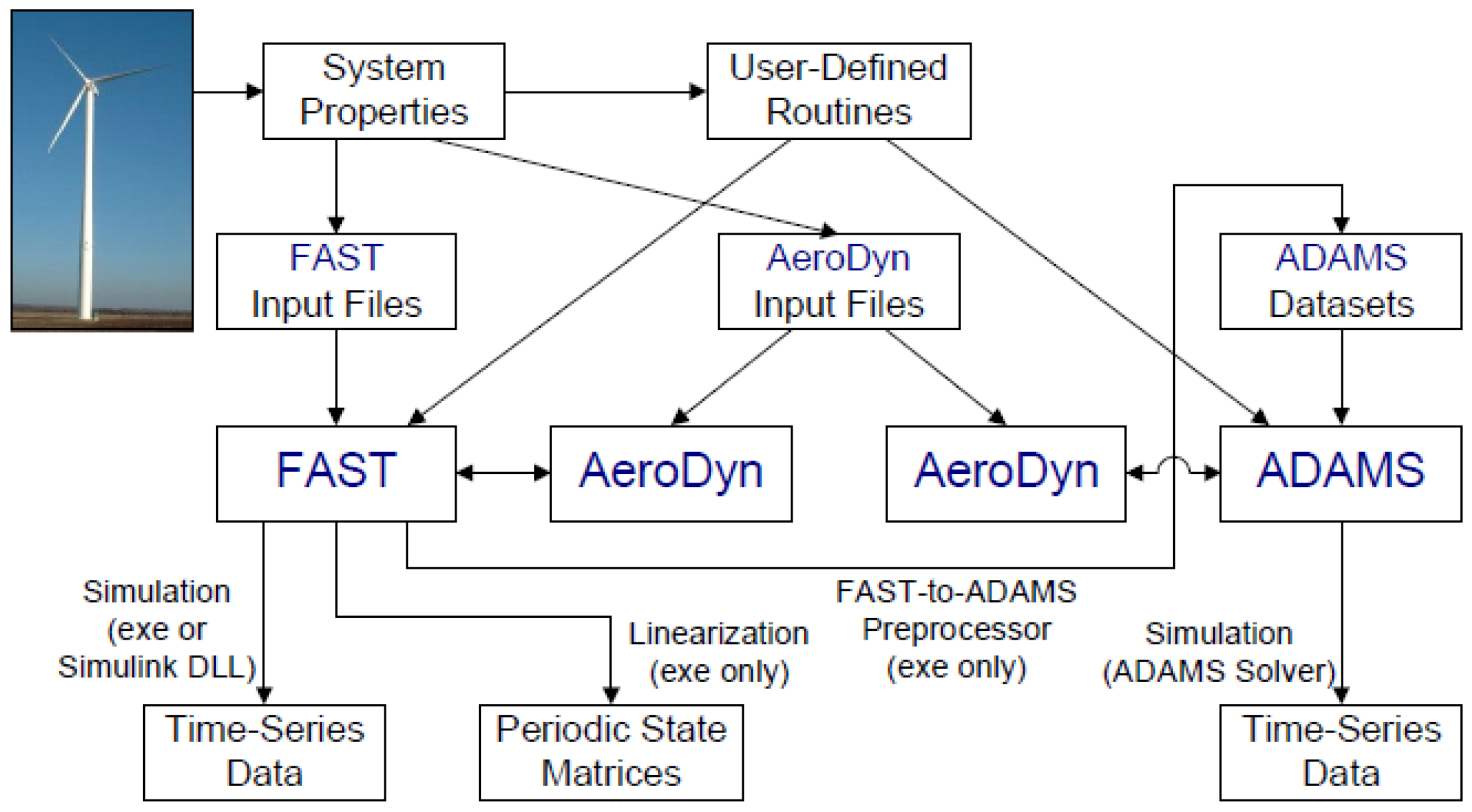
2.2. Co-Simulation Wind Turbine Interface

In this section, the interactions between the three softwares will be expounded properly to demonstrate the necessity of this interface.

The input source of wind power can be attributed to the diversity of wind conditions, which causes strength and azimuth angle differences depending on different seasons and locations on the earth. Besides, most of faulty problems such as resonance vibration and subsystem actuator shut down occur in operating periods. Besides, the control strategies in both the cut-in region and cut-out region also determine the performance of the wind turbine, which may damage the turbine if the strategy is not properly designed. All these factors show the importance of co-simulation of turbine dynamics and subsystem dynamics. The turbine dynamics software ADAMS combines the aerodynamics software FAST to present the dynamic performance in time domain. Then, the subsystem acquires the data of states such as rotor speed and pitch angle from dynamic performance, and the subsystem offers equivalent loads to drive the model. Figure 5 categorizes the roles of each software and shows the simultaneous interaction among them.

With the help of this comprehensive interface, the user can easily develop a user-based controller with desired subsystems. We not only can compare the subsystems with realistic supervisory control and data acquisition (SCADA), but create different control strategies when connecting to different types of generator or operating under different circumstances. The block diagram is presented as the structure of wind turbine configuration in Figure 6.

3. Modeling of Turbine Subsystem

The mathematic models of turbine subsystems are derived in this chapter as default model of wind turbine. A direct current (DC) motor driving pitch control system is built up in Section 3.1 and the yaw control system driven, by alternating current (AC) induction motors, is modeled in Section 3.2. Based on the design of this wind turbine, a permeant magnetic synchronized generator (PMSG) is installed without a gear box. To simplify the model, power grid and converter are simplified and implemented in Section 3.3. Finally, the maximum power point tracking (MPPT) control will be introduced in Section 4.

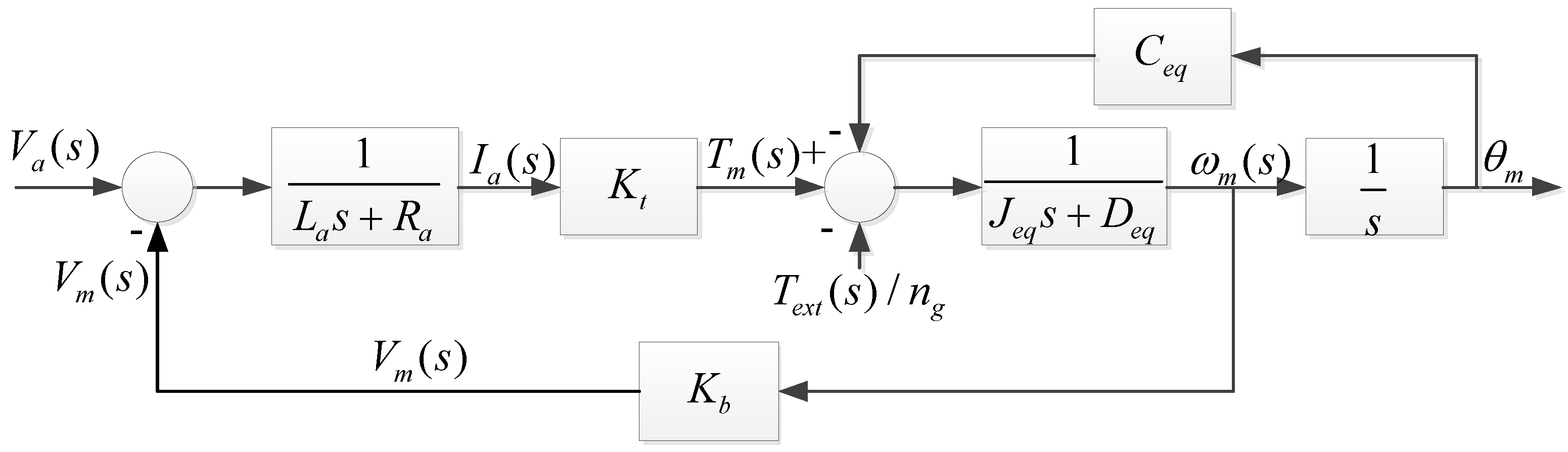
3.1. Modeling of DC Servo Motor in Pitch Control System

DC servo motors are widely used in rotatory actuator nowadays, especially in mechanical systems. The mathematic model has been developed properly and can be derived as follows:

$$V_a(t)=R_a{i}_a(t)+L_a\frac{d{i}_a(t)}{dt}+E_b$$

(4)

where $V_a$ is input voltage, $i_a$ is armature current, $R_a$ indicates armature resistance, and $R_a$ is armature inductance. $E_b$ is back electromagnetic force.

While taking gear ratio $n_g$ into consideration, the momentum equation can be rewritten as a form of rotatory angle ${\theta }_m$ and $n_g$.

$$\begin{array}{l}{\displaystyle \sum T}=n\cdot T_m-T_{ext}/n_g\\ =J_{eq}{\ddot{\theta }}_m+D_{eq}{\dot{\theta }}_m+C_{eq}{\theta }_m\\ =(J_m+\frac{J_b}{n_g^2}){\ddot{\theta }}_m+(D_m+\frac{D_b}{n_g^2}){\dot{\theta }}_m+(C_m+\frac{C_b}{n_g^2}){\theta }_m\end{array}$$

(5)

where $J_m$ refers to moment of inertia of motor, $J_b$ is moment of inertia of blades, $D_b$ is equivalent damping ratio, and $C_b$ is equivalent spring constant. Finally, the motor parameters can be estimated by the datasheet and T-n curve diagram from the supplier. For the mathematic block diagram is illustrated as Figure 7.

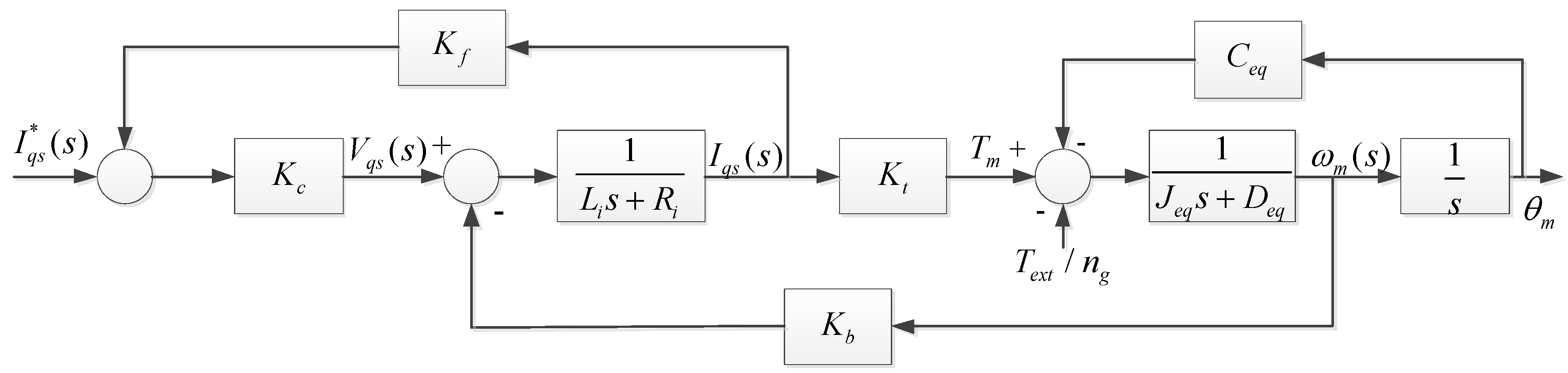
3.2. Modeling of AC Induction Motor in Yaw Control System

Induction motors are unsynchronized motors, which are usually modeled with a dynamic model using squirrel cage and reference frame, fixed on the stator [26]. The model of the induction motor can be projected to the d-q vector coordinate so that the system can be simplified as follows:

$$\left[\begin{array}{l}{v}_{ds}\\ v_{qs}\\ v_{dr}\\ v_{qr}\end{array}\right]=\left[\begin{array}{cccc}-{\omega }_s{L}_s& R_s+s{L}_s& -{\omega }_s{L}_m& s{L}_m\\ R_s+s{L}_s& {\omega }_s{L}_s& s{L}_m& {\omega }_s{L}_m\\ -{\omega }_{sl}{L}_m& s{L}_m& -{\omega }_{sl}{L}_r& R_r+L_r\\ s{L}_m& {\omega }_{sl}{L}_m& R_r+L_r& {\omega }_{sl}{L}_r\end{array}\right]\left[\begin{array}{c}{i}_{ds}\\ i_{ds}\\ i_{dr}\\ i_{qr}\end{array}\right]$$

(6)

with the electromagnetic torque is found as:

$$T_y=\frac{p}{2}\frac{3}{2}({\psi }_{qs}{i}_{ds}-{\psi }_{ds}{i}_{qs})=\frac{p}{2}\frac{3}{2}(L_m{i}_{qs}{i}_{ds}-L_m{i}_{ds}{i}_{qr})=\frac{3}{4}p{L}_m(i_{qs}{i}_{ds}-i_{ds}{i}_{qr})$$

(7)

where subtitles $ds$, $qs$, $dr$, and $qr$ are indicated as d-axis stator, q-axis stator, d-axis rotor, and q-axis rotor, respectively. $L_s$, $L_r$, and $L_m$ are the inductances of stator, rotor, and interaction. $\psi$ is the magnetic flux in each part and $p$ denotes the number of pole pairs.

As in DC motor torque control, the induction motor can be also achieved by the controlling torque and flux component independently, which is known as indirect vector control. This control is considered to be a fast response and high performance method. In the indirect vector control method, the induction motor can be operated like a separately excited DC motor for high performance applications. Likewise, many closed loop speed control techniques have been developed to improve the performance in the last decades [27].

Therefore, the system should be assumed at some ideal condition to eliminate the coupled phenomenon:

$$\begin{array}{l}{\psi }_{qr}=0\\ {\psi }_{dr}=const.\\ v_{dr}=v_{qr}=0\end{array}$$

(8)

Thus, Equations (6) and (7) can be performed by the field orientation control calculations:

$$v_{qs}=(R_s+s{L}_s)i_{qs}+{\omega }_s{L}_s{i}_{ds}+s{L}_m(-\frac{L_m}{L_r})i_{qs}$$

(9)

$$T_y=\frac{3}{4}p{L}_m(i_{qs}{i}_{ds}-i_{ds}{i}_{qr})=\frac{3}{4}p\frac{L_m^2}{L_r}{i}_{ds}{i}_{qs}=\frac{3}{4}p\frac{L_m}{L_r}{\psi }_{dr}{i}_{qs}$$

(10)

Second, the electromagnetic torque derives the mass damping system of whole nacelle with a simple torque equation with specific gear ratio $n_g$ as in Equation (5). In Figure 8, the AC induction motor is simplified as a DC servo motor block diagram.

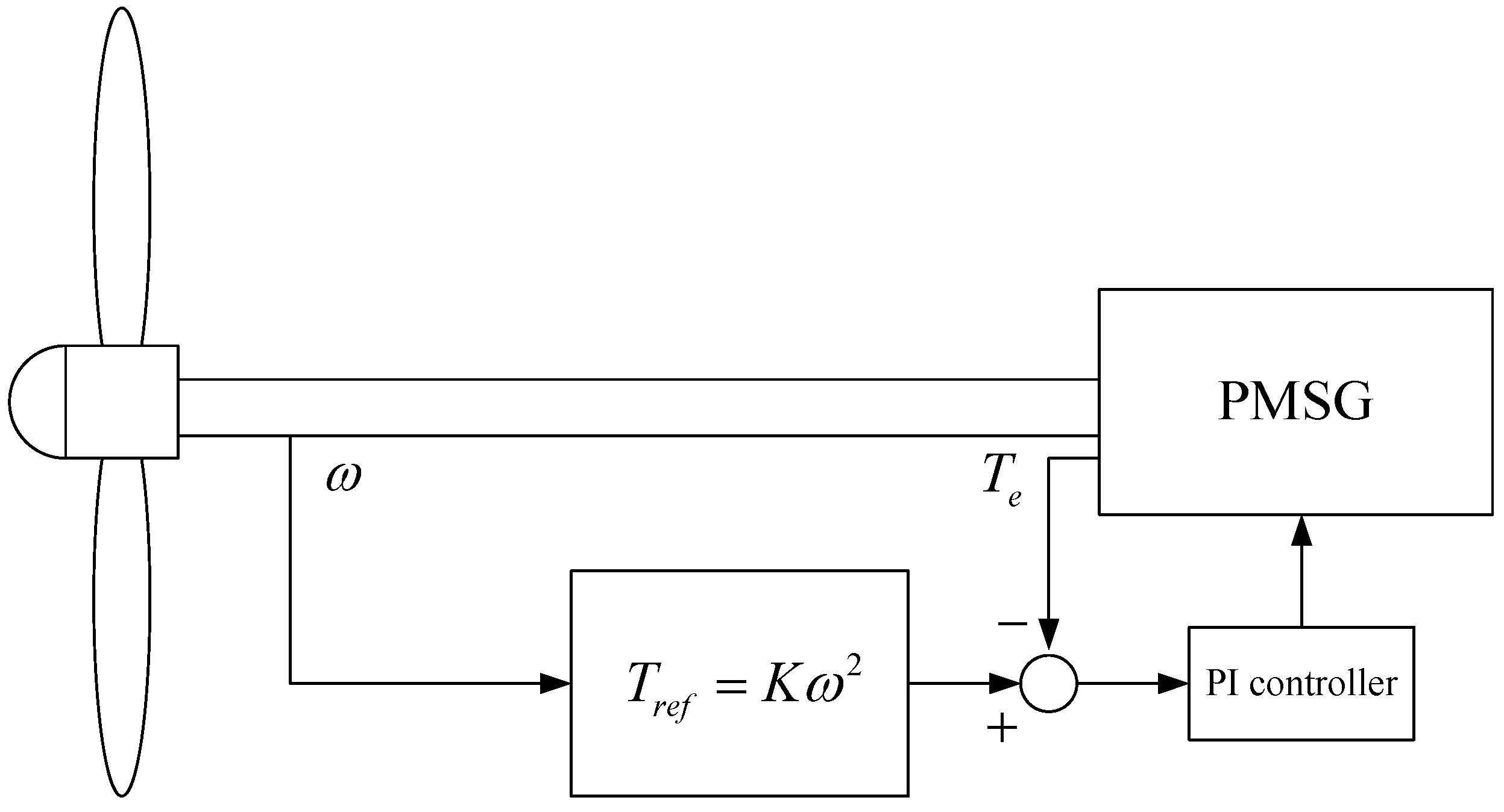
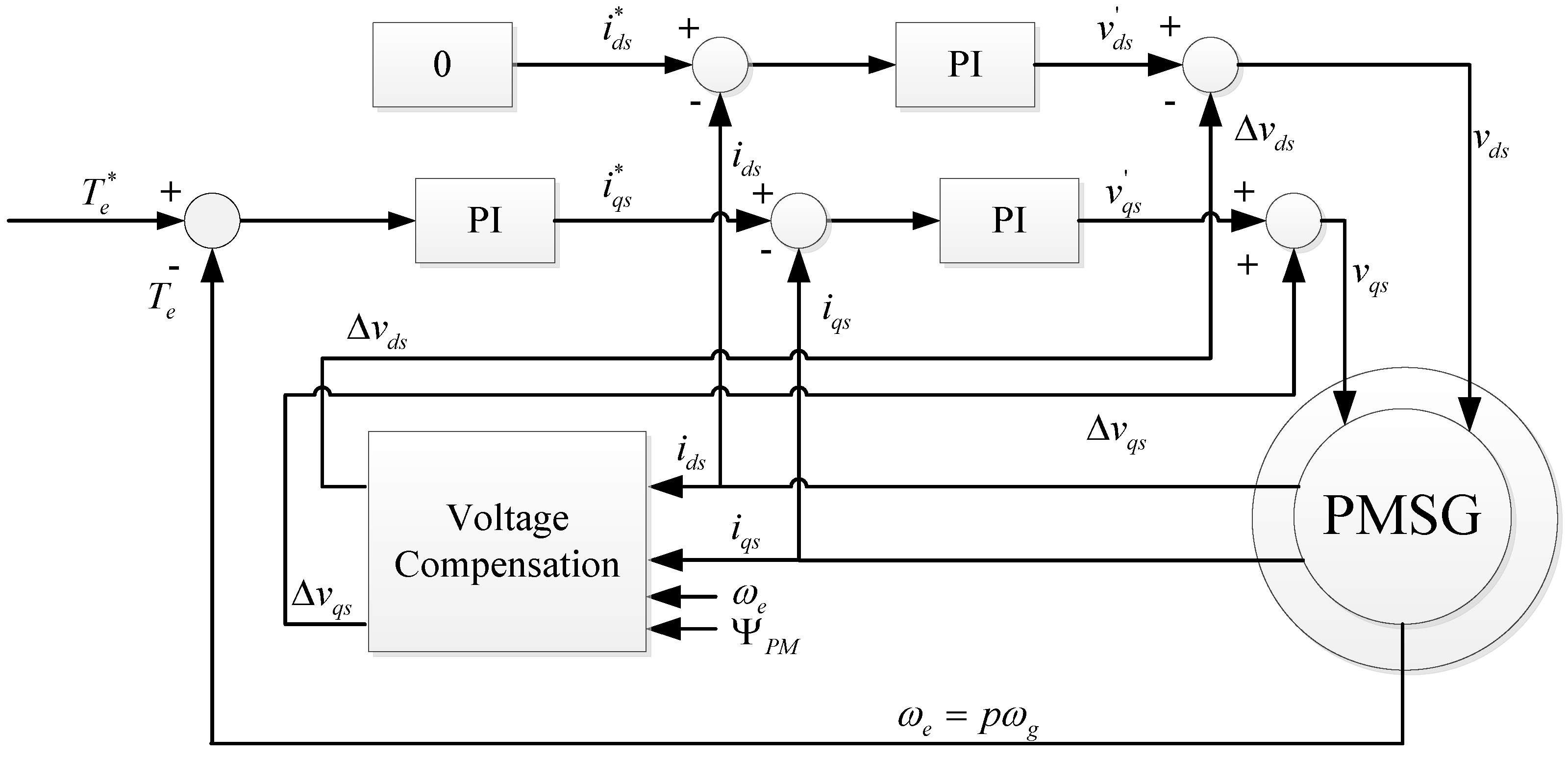
3.3. Modeling of Permanent Magnetic Synchronous Generator System

The mechanical power of the wind turbine is converted into electric power by an alternating current (AC) generator or a direct current (DC) generator. The AC generator can be either a synchronous machine or an induction (asynchronous) machine. A synchronous generator was chosen in this study with several advantages as follows: (1) the AC voltage output is synchronized with the rotor speed; (2) a synchronous generator directly connects to rotor shaft without gear sets, which can reduce not only the nacelle weights but the difficulty of installation; and (3) it offers better performance due to its higher efficiency and lower maintenance cost when comparing with double-fed induction generator. Regardless the power electric parts, this study focused neither on the converter (grid side and rotor side) nor on grid controls. The power from stator $P_s$ will be considered as power output.

The dynamic model of the PMSG is derived from the two phase (d/q) synchronous reference frame, where the q-axis is perpendicular to the d-axis along the direction of rotation. The transformation between the d-q axis rotatory reference frame and the three phase (a/b/c) frame is maintained by utilizing a phase locked loop. In order to simplify the model, magnetic hysteresis and saturation effects are negligible, and the power losses are considered as constant [28]. A form of voltage equations can be derived in Equation (11):

$$\begin{array}{l}{v}_{ds}=R_s{i}_{ds}+(L_{ds}+L_{ls})\frac{d{i}_{ds}}{dt}-{\omega }_e(L_{ds}+L_{ls})i_{qs}\\ v_{qs}=R_s{i}_{qs}+(L_{ds}+L_{ls})\frac{d{i}_{qs}}{dt}+{\omega }_e\left[(L_{ds}+L_{ls})i_{ds}+{\mathrm{\Psi }}_{PM}\right]\end{array}$$

(11)

where subscripts d/q refer to the physical quantities that have been transformed into the d/q synchronous rotating reference frame, $L_{ds}$ and $L_{ls}$ are the inductances and the leakage inductance of the stator, $i_{ds}$, $i_{qs}$ denotes the stator currents respectively, $\mathrm{R}$ is the stator resistance, ${\psi }_{PM}$ is the permanent magnetic flux, and ${\omega }_e$ is the electrical rotating speed.

Then, the mechanical load on the rotor shaft $T_g$ is equivalent with electromagnetic torque $T_e$ and it can be described by the equation as follows:

$$T_e=\frac{3}{2}p\left[{\psi }_{ds}{i}_{qs}-{\psi }_{qs}{i}_{ds}\right]=\frac{3}{2}p\left[(L_{ds}-L_{qs})i_{ds}{i}_{qs}+{\mathrm{\Psi }}_{PM}{i}_{qs}\right]$$

(12)

To avoid the risk of overvoltages due to over speeds, the stator voltage must be controlled instead of reactive power. Thus, the Field Oriented Control (FOC) strategy is implemented in the synchronous rotating reference frame for easier control [29]. This type of control also puts the PMSG into high performance. In this method, the electromagnetic equations are transformed into a coordinate system with synchronous rotation and permanent magnet flux. Besides, FOC allows separate and indirect control of the flux and torque by using a current control loop. This type of control presents several advantages such as: good torque response, accurate speed control, and achievement of full torque at zero speed. The Field Oriented Control schematic block diagram is presented in Figure 9.

Therefore, Equation (11) can be decoupled by using FOC to control $i_{ds}$ and $i_{qs}$ separately. With the help of this, Equation (11) was changed in terms of decoupled parts $\mathrm{v}$ and compensated parts $\Delta v$:

$$\begin{array}{l}{v}_{ds}=\left[R_s+(L_{ds}+L_{ls})s\right]i_{ds}-{\omega }_e(L_{ds}+L_{ls})i_{qs}={v^{\prime }}_{ds}+\Delta v_{ds}\\ v_{qs}=\left[R_s+(L_{ds}+L_{ls})s\right]i_{qs}+{\omega }_e\left[(L_{ds}+L_{ls})i_{ds}+{\mathrm{\Psi }}_{PM}\right]={v^{\prime }}_{qs}+\Delta v_{qs}\end{array}$$

(13)

Finally, in order to achieve the torque control by finding a proper torque, three PI (Proportional-Integral) controllers were used to implement FOC control. The stator current reference in d-axis must be maintained at zero to produce maximum torque which is also the usage of first controller. The stator current reference $i_{qs}^{*}$ is calculated from the reference torque using constant torque angle control property (CTA), obtained by three PI controllers. Finally, the active power $P_s$ and reactive power $Q_s$ will be determined as Equation (14):

$$\begin{array}{l}{P}_s=\frac{3}{2}[v_{ds}{i}_{ds}+v_{qs}{i}_{qs}]\\ Q_s=\frac{3}{2}[v_{qs}{i}_{ds}-v_{ds}{i}_{qs}]\end{array}$$

(14)

4. MPPT Controller Design

In this section, we demonstrate several levels of the control system. A supervisory controller with monitors is used to determine the time to start up and shut down for safety due to the wind speed data from an anemometer. Second, the mechanical performance should be controlled under the constraints of wind turbine. Torque control, which is driven by the electrical power generator, could extract a proper torque to generate an optimal power with different wind inputs. Meanwhile, the extracted torque, opposite to rotor mechanical torque driven by aerodynamics, achieves rotor speed control in some specific regions [6,10]. The pitch control should be motivated to reduce the aerodynamic loading to protect the generator from over speed when the extracted wind power exceeds the rated power. Finally, the controls of generator, including grid integration and power system, will be set as the lowest level, which is also negligible in this study.

Control Regions in Wind Turbine

As discussed in the previous paragraph, there are four different regions in a wind turbine, as shown in Figure 10. Region 1 is where the wind speed is below the cut-in speed, and pitch should keep in standby mode (90°). While the wind speed is large enough to drive the turbine but not enough to reach the rated speed, the pitch system will move to working mode for keeping 1° of pitch angle, and the turbine generator is controlled to capture the optimal power in Region 2. During Region 3, between the cut-out speed and the rated wind speed, the wind turbine reaches the maximum power capacity at rated power which is also the best region for power generation. However, if the wind exceeds the cut-out speed, the huge aerodynamic loads will damage the turbine system severely if the turbine still extracts power from the wind. Thus, the pitch control system changes the pitch angle to 90° of cut-out mode immediately in Region 4.

For the energy capture point of view, Region 2 and Region 3 are more important than others. The objective of this variable speed control in Region 2 is to extract the energy as much as possible. This can be achieved by manipulating the rotor speed to reach the optimal point in current wind input. The optimal power curve is determined by the optimal tip-speed ratio, which is the ratio between the tangential speed of the tip of a blade and the velocity of the wind, as shown in Equation (15).

$$\lambda =\frac{R\omega }{v_w}$$

(15)

The system can achieve maximum power tracking control by keeping the rotor speed at an optimal value since the optimal tip-speed ratio is fixed. However, for a large wind turbine, the slow response from the rotor shaft and the high variance of wind speed makes the system more difficult to catch the optimal rotor speed in Region 2. Thus, a torque control is developed because the extracted torque can be designed continuously to make the response smoother. This specific control law in this region is a widely used strategy in wind industry, also referred to as the ${\mathrm{K}\mathsf{\omega }}^2$ law [30,31]. In this control, the control torque can be derived as follows:

$${\tau }_c=K{\omega }^2$$

(16)

where $\mathrm{K}$ is the control gain and $\mathsf{\omega }$ is angular speed in rotor side. The control gain can be given by the combining Equation (1) with Equation (16):

$$K=\frac{{\tau }_c}{{\omega }^2}=\frac{P_w/\omega }{{\omega }^2}=\frac{1}{2}\rho A{R}^3\frac{C_{p\max }}{{\lambda }_{opt}^3},$$

(17)

In spite of tracking optimal rotor speed, this law allows the system to operate regardless the information of current wind speed. The continuous torque extracting command can also prevent the system from overloading when comparing with the speed command from optimal tip-speed ratio. Besides, this law can also still operate the turbine to the optimal operation point successfully since the optimal parameters, $C_{pmax}$ and ${\lambda }_{opt}$, have already been integrated into this control gain, which is also the constraint of this control law. The values of dominant characteristic parameters are listed in

Table 3. The dominant parameters of 2 MW wind turbine.

Name	Values	Unit
${\omega }_{rated}$	25.6771	$(rpm)$
$T_{rated}$	7.44×105	$(Nm)$
${\lambda }_{opt}$	7.37	$(-)$
$C_{p\max }$	40.08	$(\%)$

as a reference of control strategy setup, and model description and the configuration of Region 2 control is shown in Figure 11.

In Region 3, the total rotor power is much greater than rated power; unlike the double-fed induction generator with gearbox, PMSG directly links the generator to the rotor shaft. That means the synchronous generator cannot keep the rotor in rated rotating speed. In order to solve this problem, the pitch control strategy should be built to reduce the power coefficient so that the rotor can be maintained at the rated speed. In other words, the aerodynamic loading should be changed by rotating the blade pitch angle in Region 3. Meanwhile, this controller is used to implement constant generator rated power by using the pitch control algorithm. Figure 12 shows the control system configuration of maximum power tracking in Region 3.

5. Simulation Results and Comparison

This chapter contains two parts to verify the validity of the wind turbine interface and the built mathematic models. The turbine characteristics are expressed in Section 5.1 and Section 5.2 demonstrates a comparison between the measuring data of SCADA and the simulation results. In Section 5.3, mode shape analysis is recognized as another leading factor in wind turbine, thus the Campbell diagram will also be illustrated. Finally, the validity of the user-built controller strategy and the performance of real time response are shown in Section 5.4 and Section 5.5 with the $\mathrm{K}{\omega }^2$ control law and the MPPT control by implementing different kinds of wind input. Figure 13 illustrates the overall co-simulation system in MATLAB/SIMULINK, where the orange block is the interface of MATLAB/SIMULINK and ADAMS.

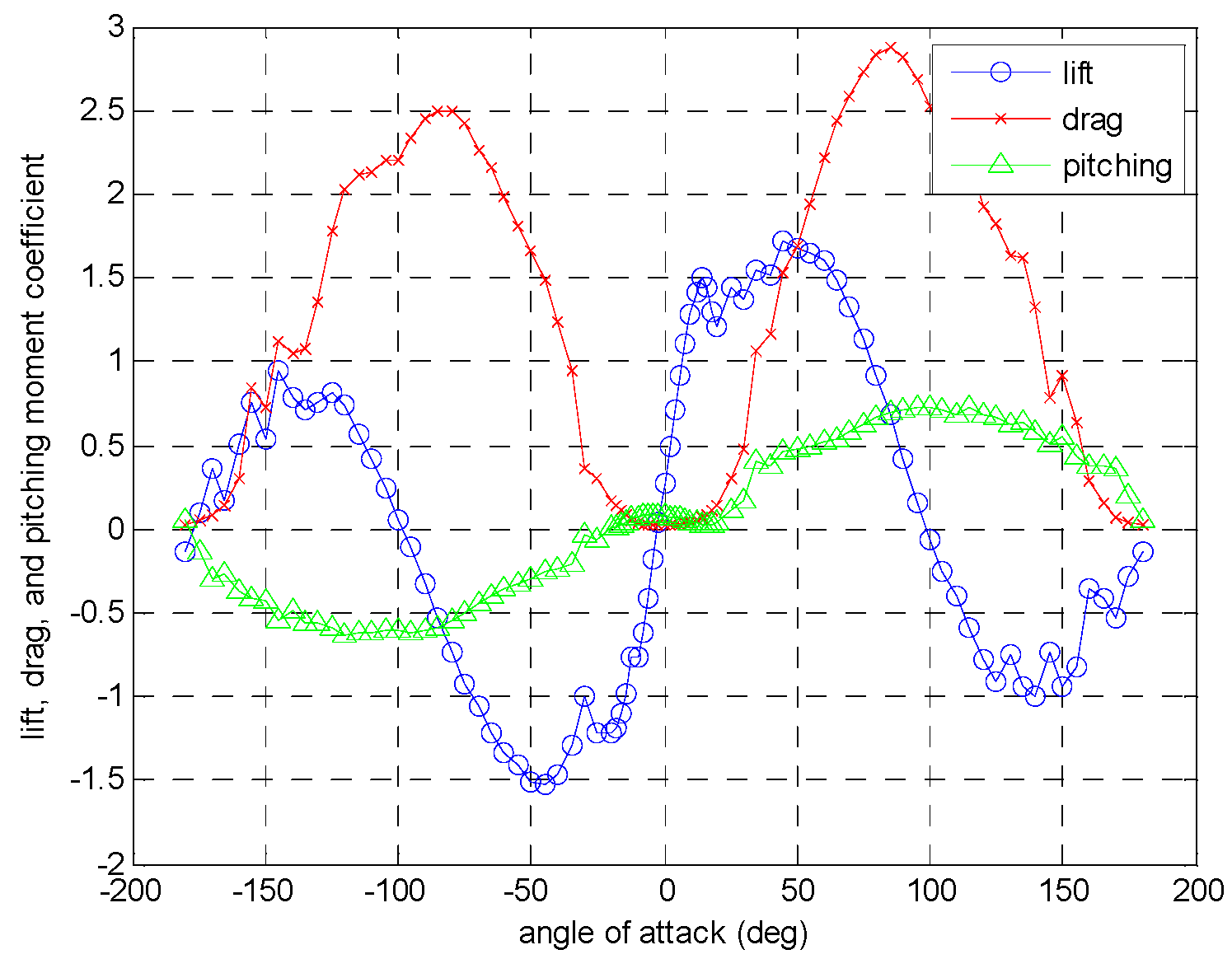
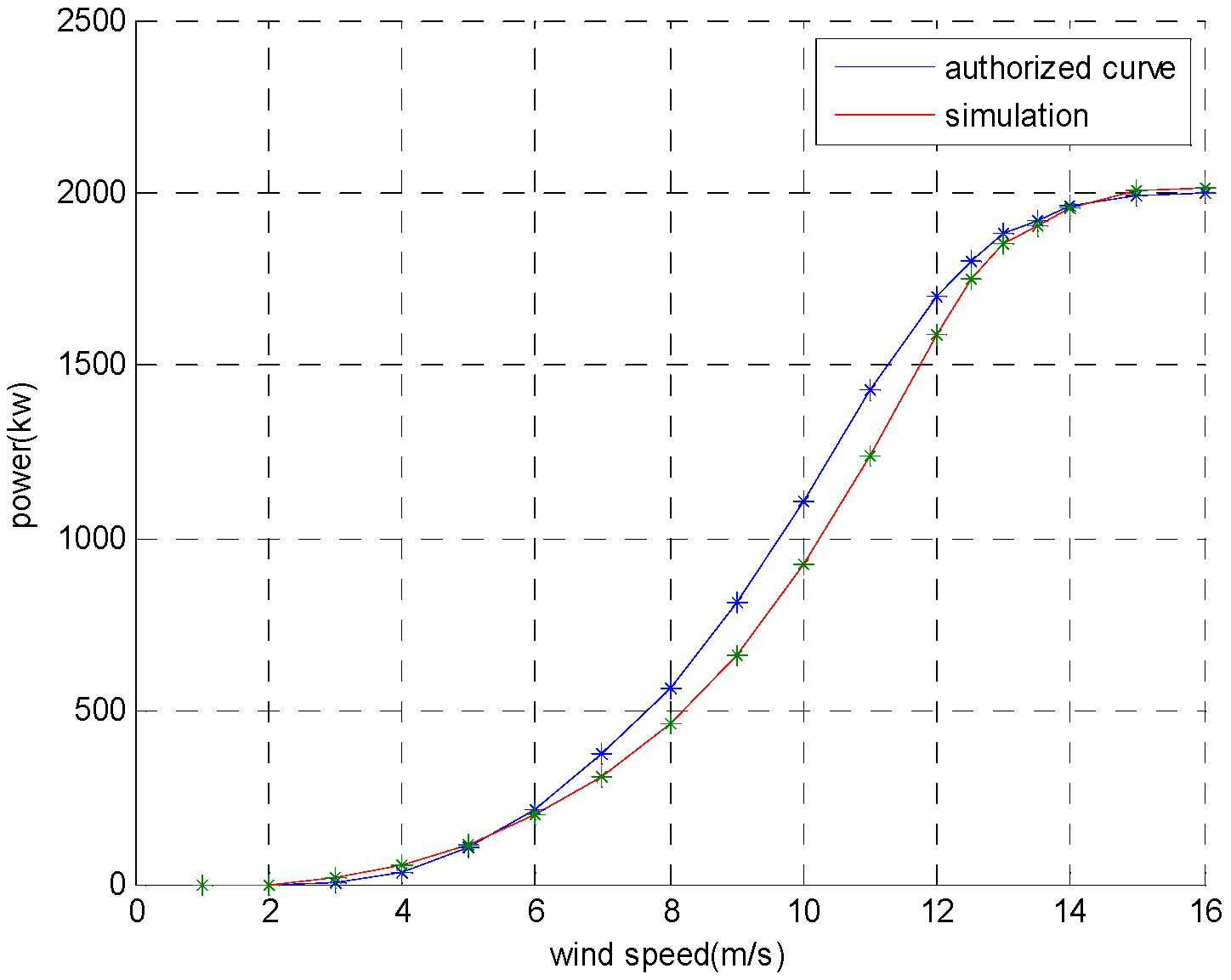
5.1. Comparison of Wind Turbine Characteristics

Performance of a wind turbine can be characterized by power curve—a graphical representation of the turbine electric power output as a function of wind speed. Based on different designs of blade airfoil and subsystem size, the power curve is recognized as an important regulation of wind turbine classification. Figure 14 denotes the comparison of the authorized power curve and the simulation power curve.

In Figure 14, the power curve of simulation is similar to the authorized curve. However, the power acquisition in middle wind speed level is below the authorized data. To explain this difference, the curve from simulation is still reasonable. Due to the wind power equation from Equation (1), wind power is proportional to the cubic of wind speed, which is also consistent with the curve in simulation (in 5 m/s and 10 m/s). Furthermore, the location of the anemometer has a strong influence on the result. In the realistic turbine, the anemometer is installed on the top of nacelle and behind the blades, which not only interferes with the accuracy of data acquisition, but also undervalues the wind due to the law of conservation of energy. This also explains why the higher the wind speed it is, the less error it is.

Meanwhile, the power coefficient can be calculated in this co-simulation modulus. If the rotor speed is too slow, most of the wind will pass through the operating area with little power extraction. On the other hand, if it is too fast, the blades will act as a solid wall to obstruct the wind flow, which also reduces the efficiency of power extraction. By determining the optimal tip-speed ratio, the control law can easily produce the optimal power with the help of power curve in Figure 14. Since the power coefficient $C_p$ will decrease after the maximum, Figure 15 illustrates the trend of power coefficient. Under a fixed and steady wind input, the theoretic power which can be extracted from a generator depends on the value of rotor speed (as generator speed). In fact, the power coefficient is a function of tip-speed ratio $\lambda$ and blade pitch angle $\beta$. By sketching the power coefficient with tip-speed ratio, the maximum of power coefficient can be captured in Figure 15, with $C_{pmax}=0.408$ with ${\lambda }_{opt}=0.737$. The formula of power coefficient can be derived in Equation (18):

$$C_p=\frac{P_g}{\raisebox{1ex}{$1$}\!\left/ \!\raisebox{-1ex}{$2$}\right.\rho A{v_w}^3}$$

(15)

where $P_g$ is the theoretical power that can be captured by the generator.

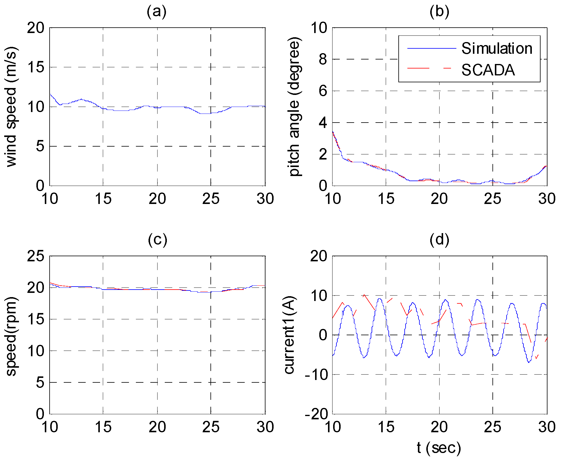
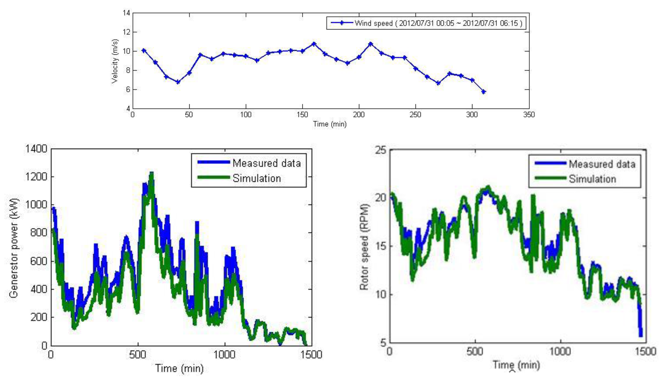
5.2. Comparison of Simulation Results with SCADA

In this section, the comparison will be divided into two parts: one is the subsystem comparison, and the other is the overall turbine comparison. The comparison in the pitch driven system of DC servo motor represents the dynamic response of the variable pitch control system. The result in Figure 16 shows the dynamic response between SCADA and simulation. By extracting the data of wind, rotor speed, and pitch angle as system input, a path trajectory control was used to catch up the desired pitch angle. The result shows a good performance in path trajectory control, and dynamic response of motor torque is correspondent with the SCADA. However, there are the constraints in computational calculations that may cause certain error between the simulation and the SCADA. Some possible reasons are environmental parameters mismatch, such as azimuth and tilt angle of the input wind profile.

Second, the overall data comparison denotes the overall efficiency between the realistic turbine and simulation model. The wind input will also be shown in this case to express the realistic wind profile in Taiwan. Figure 16 is a comparison of pitch system in a short-term time response and Figure 17 makes a long-term time response comparison of turbine dynamics and power output. The results of Figure 16 and Figure 17 show the reliability and major consistence between simulation model and SCADA. Thus, this integrated co-simulation methodology can be recognized as a convincing tool for dynamic simulation.

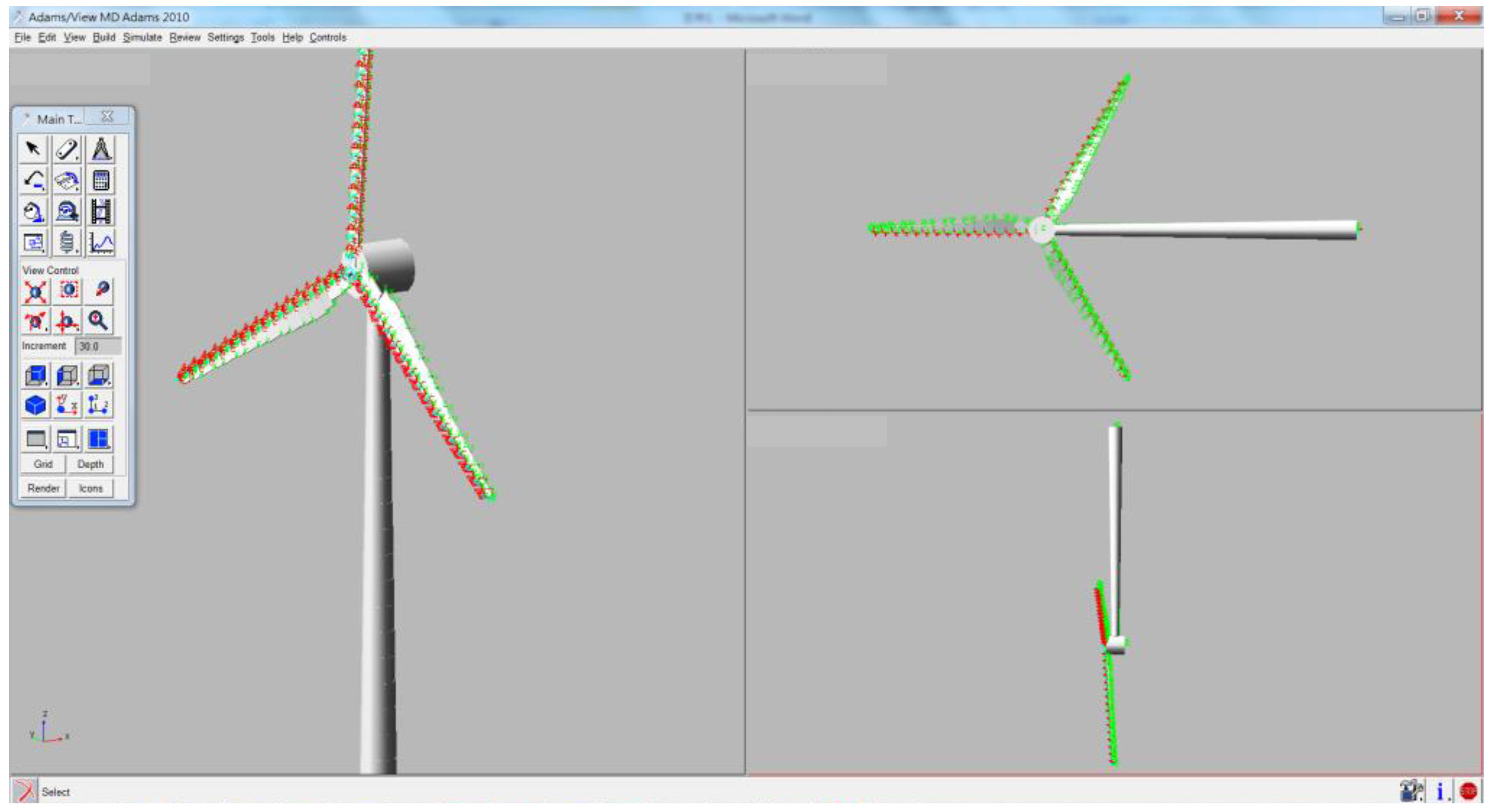
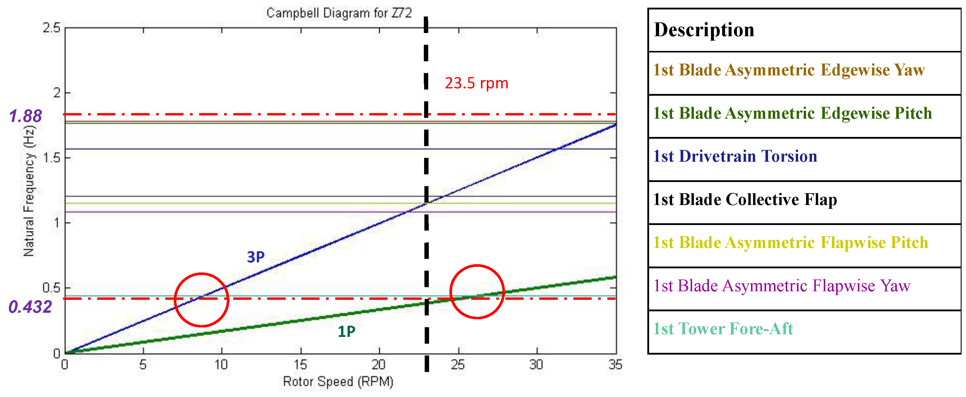
5.3. Mode Shape Analysis of Wind Turbine

The significant resonance phenomenon of the wind turbine system can be observed when the structural frequencies match with the frequency resulting from mass unbalance of blades or the harmonic frequencies due to blade passage of tower, which is also known as tower shadow. Other external loads such as low frequency sea wave or earthquake hitting on the tower base will also produce the resonance in many issues. Maintaining activation of the resonance phenomenon will lead to structural deformation and create fatigue in the tower [32]. In order to increase the lifetime and reduce the cost of maintenance, the resonance frequency should be avoided by adding rule-based controller strategies. All these reemphasize the importance of mode shape analysis.

Table 4. Comparison of blade tower mode shape analysis.

Tower	1st fore-aft	2nd fore-aft
Experiment	0.432	3.281
ADAMS	0.441	3.813
Blade	1st fore-aft	2nd fore-aft
Experiment	1.880	3.000
ADAMS	1.151	3.193

shows the comparison of different mode frequencies by ADAMS analysis and practical experimental measurement.

With the help of this interface, a Campbell diagram can be developed in design and analysis, as shown in Figure 18. By sketching the curve of different mode frequencies versus rotating speed, the resonance point of frequency can be determined and forecasted beforehand, as the red circles shown in Figure 18. At approximately 26.5 rpm, blade 1P hit the first tower fore–aft frequency, which is also observed in the real time. Thus, we can create a rule-based control strategy depending on different model of wind turbine with the help if this Campbell diagram.

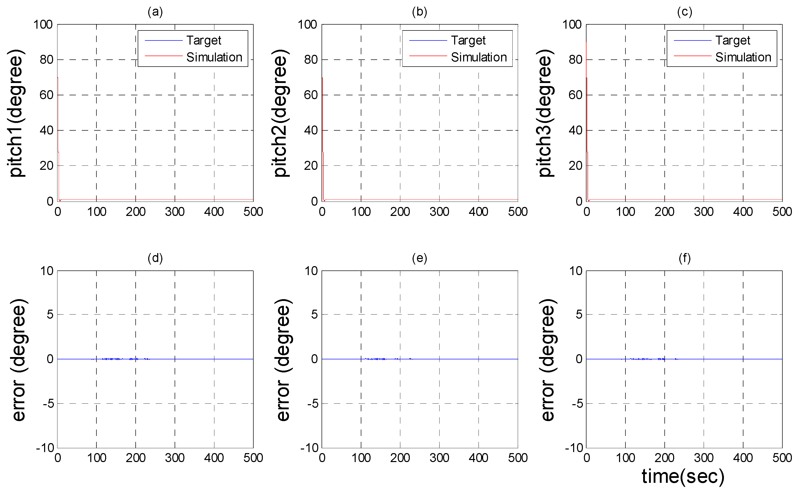
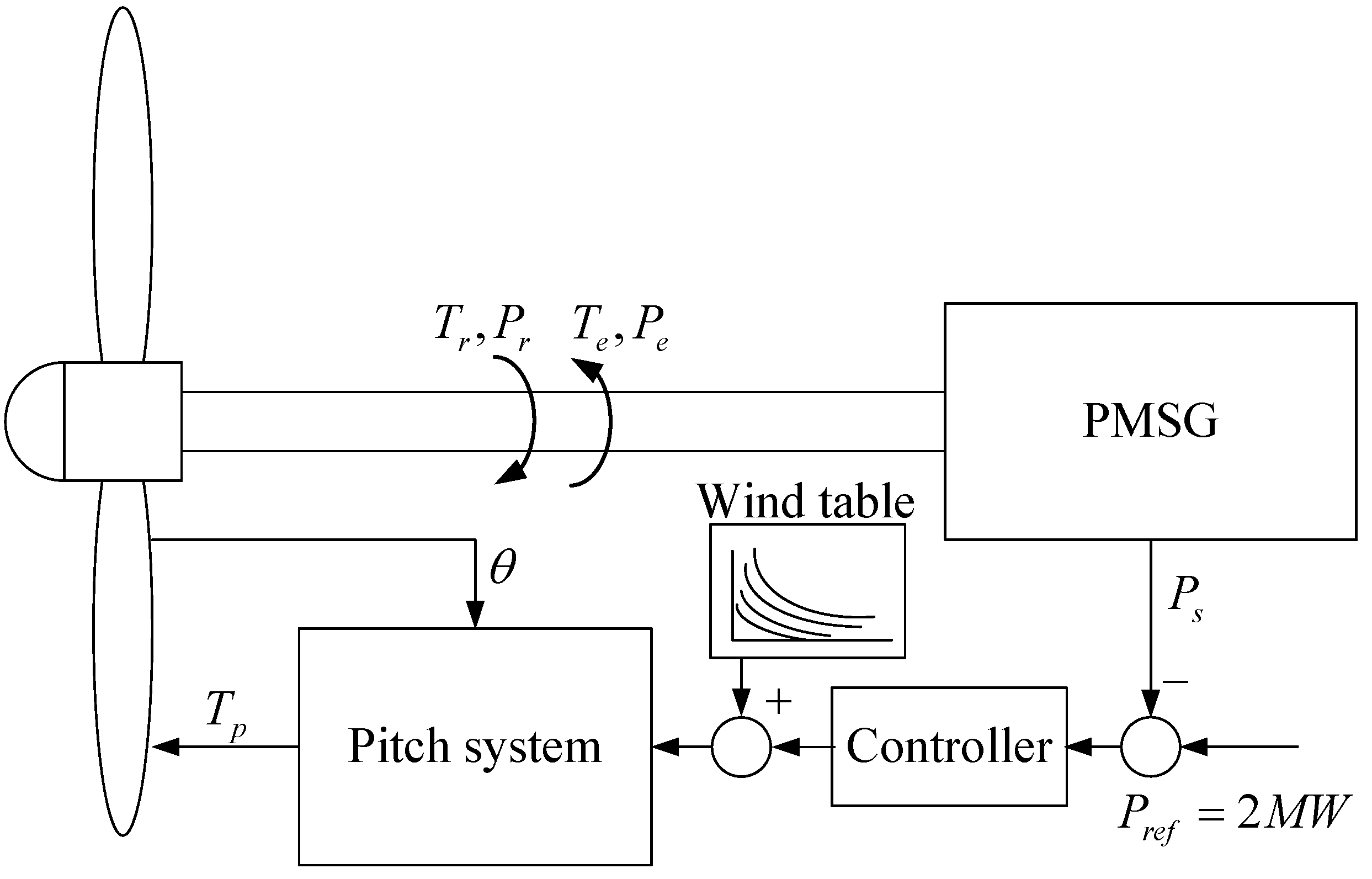
5.4. Overall Simulation in Region 2

Owing to $\mathrm{K}{\omega }^2$ law shown in Section 4, torque can be extracted smoothly under randomly fluctuating wind conditions. In Figure 19, pitch angle starts from standby condition to working condition, then the power extraction is activated when the rotational speed exceeds the cut-in speed, which is the optimal rotor speed calculated by cut-in wind speed (3 m/s). Under rated wind speed, the control strategy follows the $\mathrm{K}{\omega }^2$ law to generate the power depending on the current rotor speed. Although the generator could not reach the optimal rotor speed in real-time response, the system drops the total efficiency to prevent the impulsive loading when encountering a sudden wind discrepancy. The difference between optimal rotor speed and simulation data are shown in Figure 20b,c. Finally, the overall efficiency and the simulation wind profile are expressed in Figure 21. Obviously, the optimal power tracking has been implemented according to the $\mathrm{K}{\omega }^2$ law. However, some errors, such as the overestimated power coefficient, can result from following reasons: (1) the drop of power coefficient in the beginning is owing to system start up with zero rotational speed and (2) the values that are much larger than the maximum power coefficient are caught by the sudden changes of wind conditions that the response from the rotor could not react to immediately.

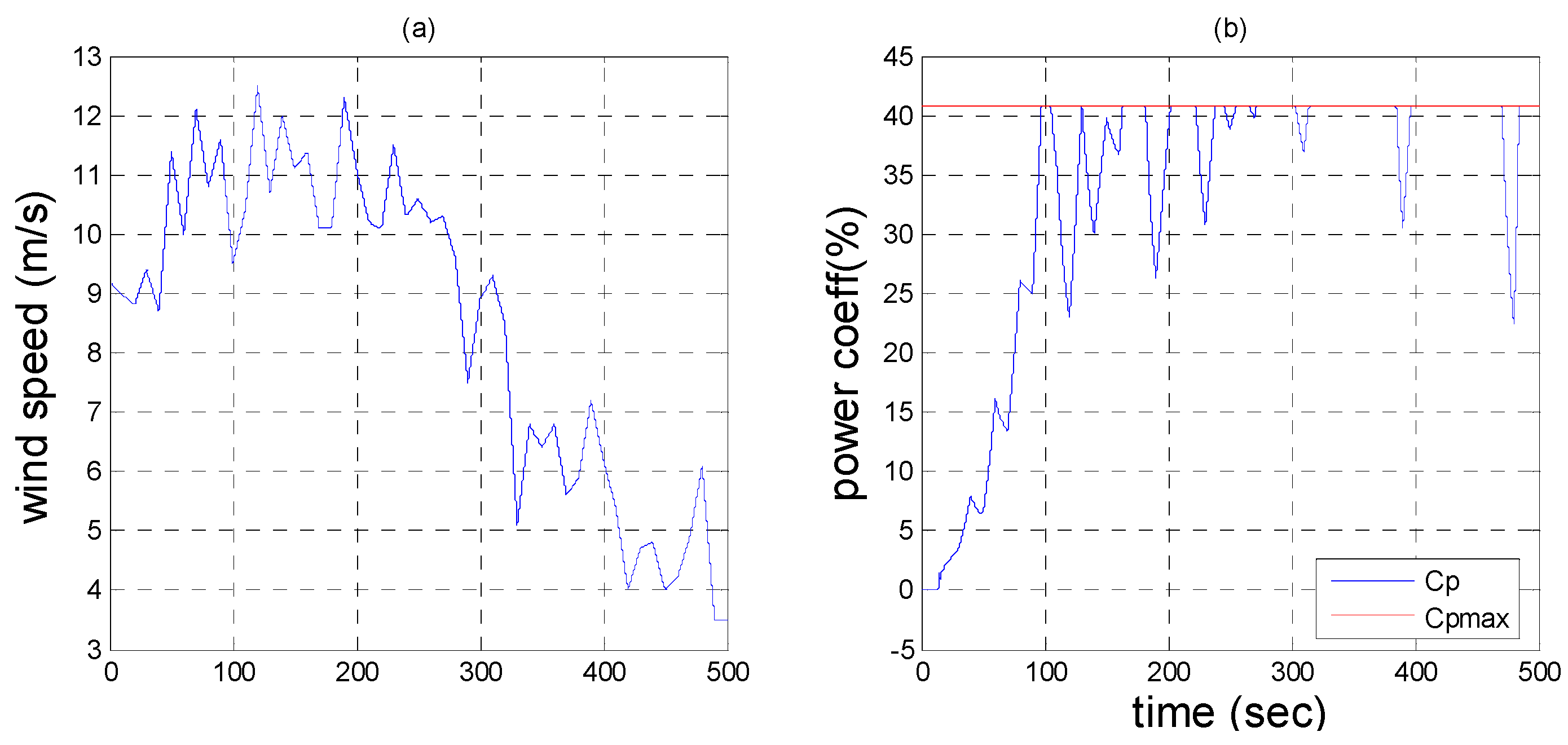
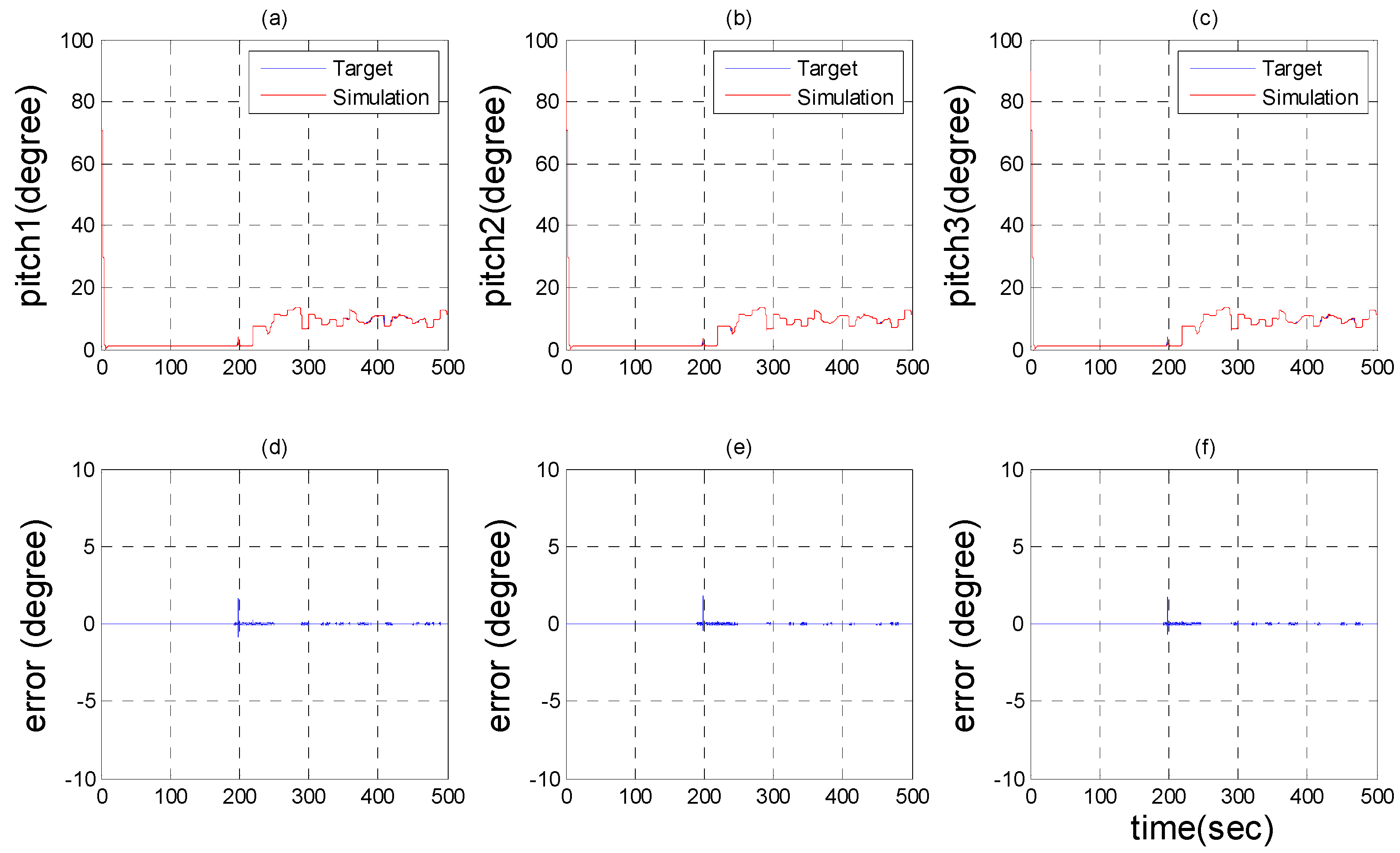
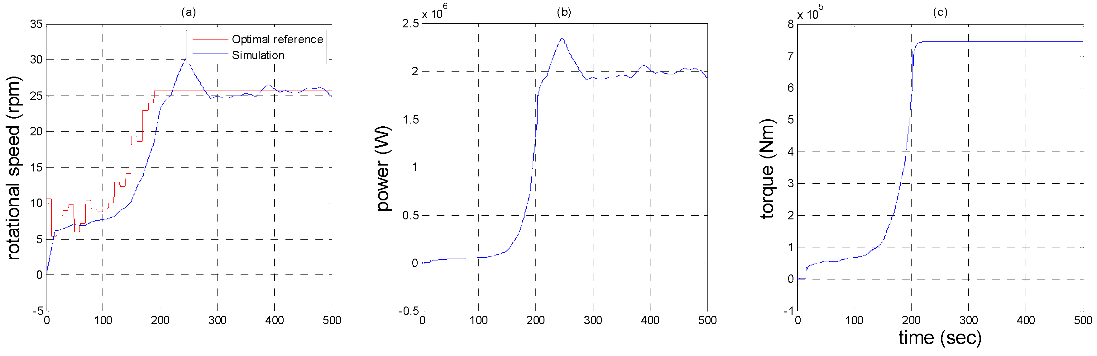
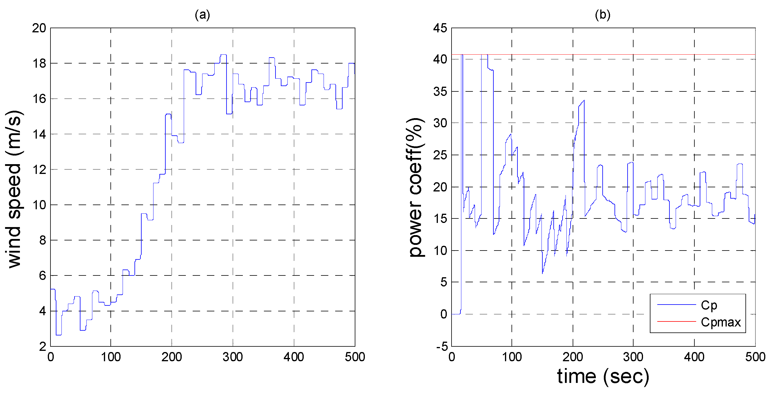
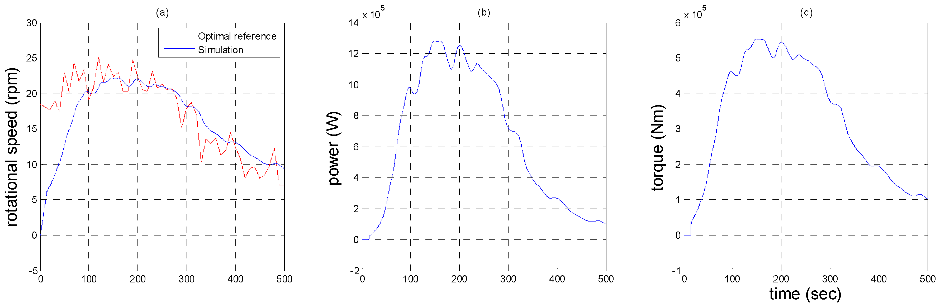
5.5. Overall Simulation of MPPT

In order to achieve the maximum power tracking control, a proper control strategy in Region 3 is necessary. In this region, the power has reached the rated power due to the sufficient aerodynamics loads. The exceeded power should be released to prevent the overloading and the damage to PMSG generator. The $\mathrm{K}{\omega }^2$ law still operates until rotor speed reaches the rated rotor speed to achieve optimal power tracking control. Then, variable pitch system is activated when output power is going to overrated power (2 MW). In Figure 22, pitch actuator starts functioning from 220 s. The pitch reference is changed with the help of wind table which is built up in advanced and compensated by a PID controller to smooth the trajectory for the discontinuity. The rotor speed difference in Figure 23a follows the optimal tip-speed ratio well and performs the variable speed control successfully, and the output power in Figure 23b,c expresses the control strategy and the simulation successfully, presenting maximum power tracking control in this co-simulation interface. An overspeed can result from a sudden rise of the wind input (12 m/s to 18 m/s) in Figure 24a. Under this condition, the power coefficient must be below the maximum value to prevent the damage in Figure 24.

6. Conclusions

The paper not only proposed a novel co-simulation system of wind turbines combining three advanced softwares, but also built up a comprehensive data comparison with a real wind turbine. Each software played a different role in the simulation to achieve an overall system dynamic response. Meanwhile, in order to present the dynamic response of the wind turbine, three subsystems such as DC servo pitch driven motor, AC induction yaw driven motor, and one directly driven permanent magnetic synchronous generator were built up to drive the components simultaneously. Besides, a system controller with control strategies was set up to achieve the optimal power tracking control with $\mathrm{K}{\omega }^2$ law. The simulation results in different regions proved the system controller worked perfectly in a correct mode with a good response. Finally, the parameters of each subsystem were adjusted through SCADA comparison to ensure the reliability of this simulation.

References

1. Burton, D.S.T.; Jenkins, N.; Bossanyi, E. Wind Energy Handbook; John Wiley &sons Ltd.: Chichester, UK, 2001. [Google Scholar]
2. Wang, Y.; Li, Q.; Qin, S. A new method of wind turbines modeling based on combined simulation. In Proceedings of the 2014 International Conference on Power System Technology (POWERCON), Chengdu, China, 20–22 October 2014.
3. MATLAB Homepage. Available online: http//www.mathworks.com (accessed on 17 June 2016).
4. Younsi, R.; El-Batanony, I.; Tritsch, J.-B.; Naji, H.; Landjerit, B. Dynamic study of a wind turbine blade with horizontal axis. Eur. J. Mech. A Solids 2010, 20, 241–252. [Google Scholar] [CrossRef]
5. Howell, R.; Qin, N.; Edwards, J.; Durrani, N. Wind tunnel and numerical study of a small vertical axis wind turbine. Renew. Energy 2010, 35, 412–422. [Google Scholar] [CrossRef]
6. Wilmshurst, S.M.B. Control Strategies for Wind Turbines; National Renewable Energy Laboratory: Washington, DC, USA, 1988. [Google Scholar]
7. Freeman, J.B.; Balas, M.J. An investigation of variable speed horizontal-axis wind turbines using direct model-reference adaptive control. In Proceedings of the 18th ASME (American Society of Mechanical Engineers) Wind Energy Symposium, Reno, NV, USA, 11–14 January 1999.
8. Jones, R.; Smith, G.A. High quality mains power from variable-speed wind turbines. In Proceedings of the 2001 International Conference on Renewable Energy—Clean Power, London, UK, 17–19 November 1993.
9. Idan, M.; Lior, D. Continuously variable speed wind turbine: Transmission concept and robust control. Wind Eng. 2000, 24, 151–167. [Google Scholar] [CrossRef]
10. Song, Y.D.; Dhinakaran, B.; Bao, X.Y. Variable speed control of wind turbines using nonlinear and adaptive algorithms. J. Wind Eng. Ind. Aerodyn. 2000, 85, 293–308. [Google Scholar] [CrossRef]
11. Boukhezzar, B.; Siguerdidjane, H. Nonlinear control of variable speed wind turbines without wind speed measurement. In Proceedings of the 44th IEEE Conference on Decision Control/European Control Conference (CCD-ECC), Seville, Spain, 12–15 December 2005.
12. Camblong, H.; Tapia, G.; Rodriguez, M. Robust digital control of a wind turbine for rated-speed and variable-power operation regime. Control Theory Appl. IEE Proc. 2006, 153, 81–91. [Google Scholar] [CrossRef]
13. Felippa, C.A.; Park, K.C.; Farhat, C. Partitioned analysis of coupled mechanical systems. Comput. Methods Appl. Mech. Eng. 2001, 190, 3247–3270. [Google Scholar] [CrossRef]
14. Boukhezzar, B.; Lupu, L.; Siguerdidjane, H.; Hand, M. Multivariable control strategy for variable speed, variable pitch wind turbines. Renew. Energy 2007, 32, 1273–1287. [Google Scholar] [CrossRef]
15. Zhang, J.; Cheng, M.; Chen, Z. Design of wind turbine controller by using wind turbine codes. In Proceedings of the 11th International Conference on Electrical Machines and Systems, Wuhan, China, 17–20 October 2008.
16. Fadaeinedjad, R.; Moschopoulos, G.; Moallem, M. Simulation of a wind turbine with doubly-fed induction machine using FAST and Simulink. In Proceedings of the 2006 IEEE International Symposium on Industrial Electronics, Montreal, Canada, 9–13 July 2006.
17. Lu, R.K.; Chang, C.R. Load Computation of a 150 kW wind turbine by IEC-61400-1via FAST/SIMULINK. In Proceedings of the Taiwan Wind Energy Conference, Taipei, Taiwan, 1–6 December 2009.
18. Mandic, G.; Nasiri, A. Modeling and simulation of a wind turbine system with ultracapacitors for short-term power smoothing. In Proceedings of the 2010 IEEE International Symposium on Industrial Electronics (ISIE), Bari, Italy, 4–7 July 2010.
19. Sicklinger, S.; Lerch, C.; Wüchner, R.; Bletzinger, K.-U. Fully coupled co-simulation of a wind turbine emergency brake maneuver. J. Wind Eng. Ind. Aerodyn. 2015, 144, 134–145. [Google Scholar] [CrossRef]
20. Sicklinger, S.A. Stabilized Co-Simulation of Coupled Problems Including Fields and Signals. Ph.D. Thesis, Technische Universität München, München, Gemany, 2014. [Google Scholar]
21. Anis, A. Simulation of slider crank mechanism using Adams software. Int. J. Eng. Technol. 2012, 12, 108–112. [Google Scholar]
22. Jingjun, Z.; Jitao, Z.; Ruizhen, G.; Lili, H. The application of co-simulation technology of ANSYS and MSC.ADAMS in structural engineering. In Proceedings of the 2010 International Conference on Mechanic Automation and Control Engineering (MACE), Wuhan, China, 26–28 June 2010.
23. Li, T.; Zhang, J.; Chen, D.F.; Zhang, Z.; Hu, J. Dynamics researches of megawatt wind turbine gear increaser based on Adams. In Proceedings of the 2011 6th International Conference on Pervasive Computing and Applications (ICPCA), Port Elizabeth, South Africa, 26–28 October 2011.
24. Bak, C.A.M.; Aagaard, H.; Johansen, J. Influence from blade-tower interaction on fatigue loads and dynamics (poster). In Proceedings of the Wind energy for the new millennium, Copenhagen, Denmark, 2–7 July 2001.
25. Jonkman, J.M.; Buhl, M.L., Jr. FAST User’s Guide; National Renewable Energy Laboratory: Washington, DC, USA, 2005. [Google Scholar]
26. Uddin, M.N.; Radwan, T.S.; Azizur Rahman, M. Performances of fuzzy-logic-based indirect vector control for induction motor drive. Ind. Appl. IEEE Trans. 2002, 38, 1219–1225. [Google Scholar] [CrossRef]
27. Gaeid, K.S.; Hew, P.; Mohamed, H.A.F. Indirect vector control of a variable frequency induction motor drive (VCIMD). In Proceedings of the 2009 International Conference on Instrumentation, Communications, Information Technology, and Biomedical Engineering (ICICI-BME), Bandung, Indonesia, 23–25 November 2009.
28. Rolan, A.; Luna, A.; Vazquez, G.; Aguilar, D.; Azevedo, G. Modeling of a variable speed wind turbine with a Permanent Magnet Synchronous Generator. In Proceedings of the IEEE International Symposium on Industrial Electronics (ISIE 2009), Seoul, Korea, 5–8 July 2009.
29. Busca, C.; Stan, A.I.; Stanciu, T.; Stroe, D.I. Control of Permanent Magnet Synchronous Generator for large wind turbines. In Proceedings of the 2010 IEEE International Symposium on Industrial Electronics (ISIE), Bari, Italy, 4–7 July 2010.
30. Merabet, A.; Thongam, J.; Gu, J. Torque and pitch angle control for variable speed wind turbines in all operating regimes. In Proceedings of the 2011 10th International Conference on Environment and Electrical Engineering (EEEIC), Rome, Italy, 8–11 May 2011.
31. Johnson, E.; Balas, M.J.; Pao, L.Y. Methods for increasing region 2 power capture on a variable speed HAWT. In Proceedings of the 23rd ASME (American Society of Mechanical Engineers) Wind Energy Symposium, Reno, NV, USA, 5–8 January 2004.
32. Hu, W.H.; Sebastian, T.; Samir, S.; Werner, R. Resonance phenomenon in a wind turbine system under operational conditions. In Proceedings of the 9th International Conference on Structural Dynamics, Porto, Portugal, 30 June–2 July 2014.
Figure 1. Co-simulation of FAST (aerodynamics), ADAMS (mechanism dynamic), and MATLAB/SIMULINK (subsystems and control system) for wind turbines.
Energies 09 00637 g001
Figure 2. Lift and drag force of blade airfoil.
Energies 09 00637 g002
Figure 3. Lift, drag, and pitching moment coefficients at 17,750 mm based on the blade root.
Energies 09 00637 g003
Figure 4. 3D expression of wind turbine outlook.
Energies 09 00637 g004
Figure 5. Interaction between each software [25].
Energies 09 00637 g005
Figure 6. Block diagram of wind turbine system configuration.
Energies 09 00637 g006
Figure 7. Block diagram of DC servo motor.
Energies 09 00637 g007
Figure 8. Block diagram of alternating current (AC) induction motor.
Energies 09 00637 g008
Figure 9. Block diagram of field oriented control.
Energies 09 00637 g009
Figure 10. Four control regions in a wind turbine.
Energies 09 00637 g010
Figure 11. Control system configuration in Region 2.
Energies 09 00637 g011
Figure 12. Control system configuration in Region 3.
Energies 09 00637 g012
Figure 13. Overall co-simulation system in MATLAB/SIMULINK.
Energies 09 00637 g013
Figure 14. Power curve comparison of the practical wind turbine and the simulation.
Energies 09 00637 g014
Figure 15. Power coefficient of wind turbine in function of tip speed ratio.
Energies 09 00637 g015
Figure 16. Pitch subsystem comparison of 2 MW wind turbine: (a) Input wind; (b) Pitch angle; (c) Rotor speed; and (d) Motor current.
Energies 09 00637 g016
Figure 17. Overall comparison of 2 MW wind turbine: 2012/07/31 00:05–06:15.
Energies 09 00637 g017
Figure 18. Campbell diagram of 2 MW wind turbine.
Energies 09 00637 g018
Figure 19. Pitch angle tracking control in region 2: (a) Pitch 1; (b) Pitch 2; (c) Pitch 3; (d) Pitch 1 tracking error; (e) Pitch 2 tracking error; (f) Pitch 3 tracking error.
Energies 09 00637 g019
Figure 20. Generator performance in Region 2: (a) Generator speed; (b) Output power; (c) Electromagnetic torque.
Energies 09 00637 g020
Figure 21. Wind input and overall efficiency in Region 2: (a) Wind input; (b) Overall power coefficient.
Energies 09 00637 g021
Figure 22. Pitch angle tracking control in Region 3: (a) Pitch 1; (b) Pitch 2; (c) Pitch 3; (d) Pitch 1 tracking error; (e) Pitch 2 tracking error; (f) Pitch 3 tracking error.
Energies 09 00637 g022
Figure 23. Generator performance in Region 3: (a) Generator speed; (b) Output power; (c) Electromagnetic torque.
Energies 09 00637 g023
Figure 24. Wind input and overall efficiency in Region 3: (a) Wind input; (b) Overall power coefficient.
Energies 09 00637 g024