
Energy Management in Prosumer Communities: A Coordinated Approach


Abstract
:
1. Introduction
2. Preliminaries: Government Policies, Markets and Management Paradigms
2.1. Government Policies and Market Structure
2.2. Energy Management Paradigms
2.2.1. Demand Management Strategies
Demand Management from the Supply-Side
- Event-based: an aggregator remotely controls appliances (and the associated loss or gain in QoL), with the control taking place at particular events. Examples include direct load control, emergency programs, curtailment programs, and demand bidding programs.
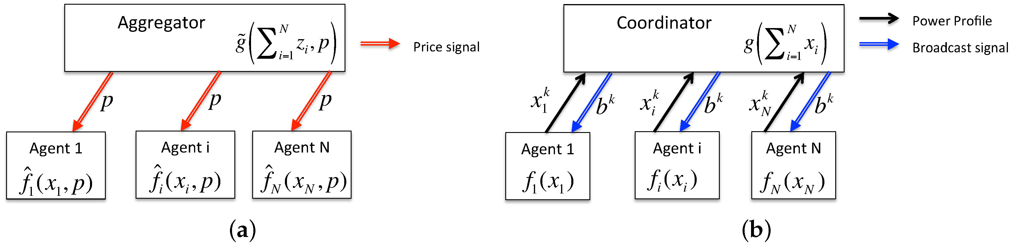
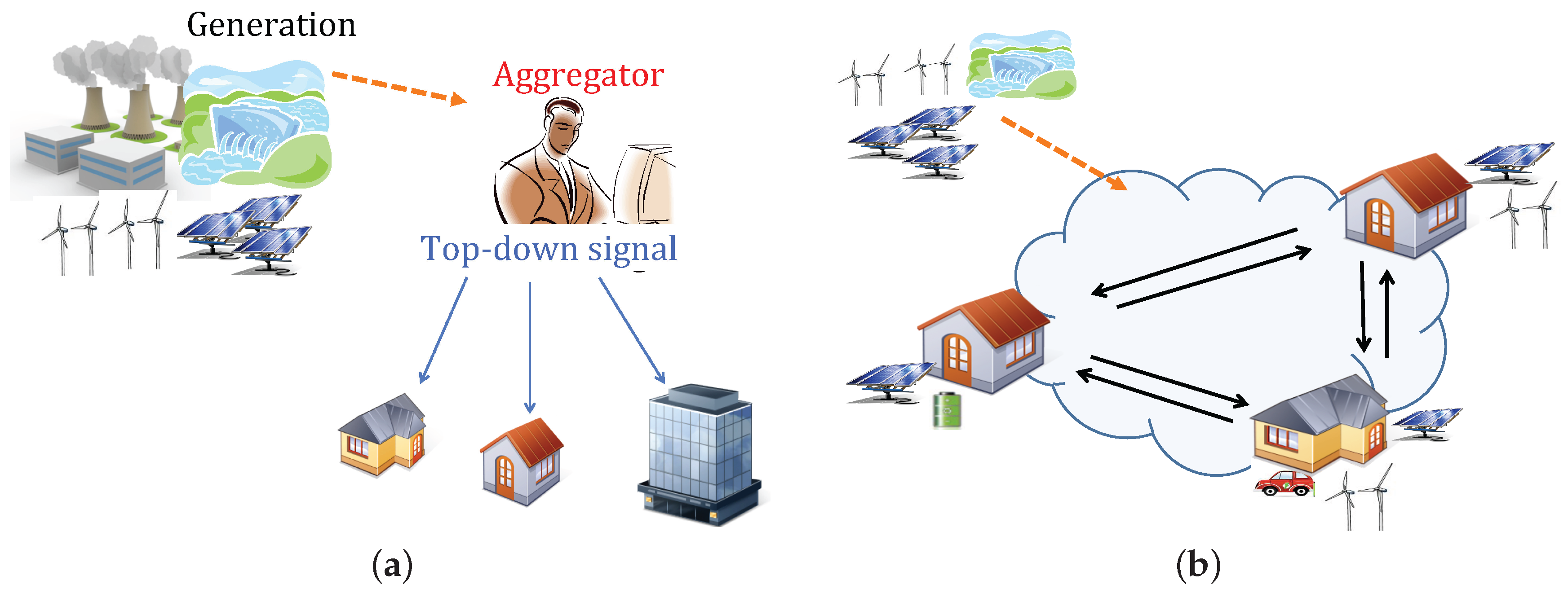
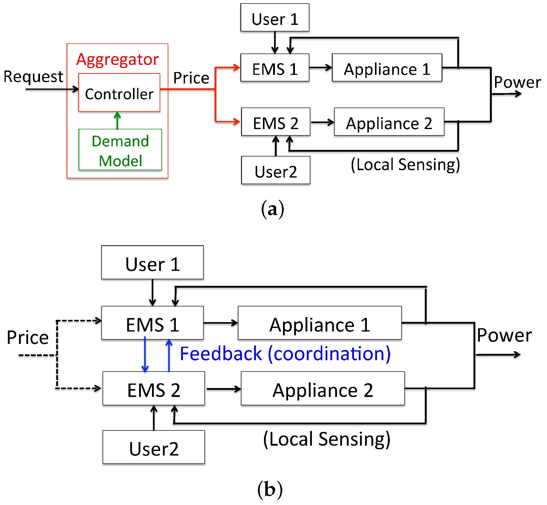
- Price-based: an aggregator sends the same price-signal to all users, seeking to modify their consumption patterns. Based on the price signal, each user independently decides its power usage. Examples include time-of-use (TOU), critical-peak-pricing (CPP), and real-time-pricing (RTP).
Demand Management from the Demand-Side
- They do not consider a common goal for the group, but just the goal of each agent in the group.
- They consider not only the management of the demand, but also the management of the grid (transmission, distribution, and energy hubs). Whereas managing the grid is important, we think the energy management of the demand should be done independently of the underlying grid.
2.3. Coordinated Energy Management
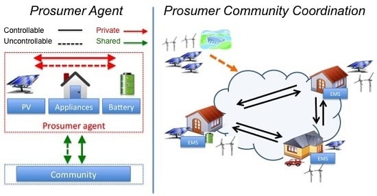
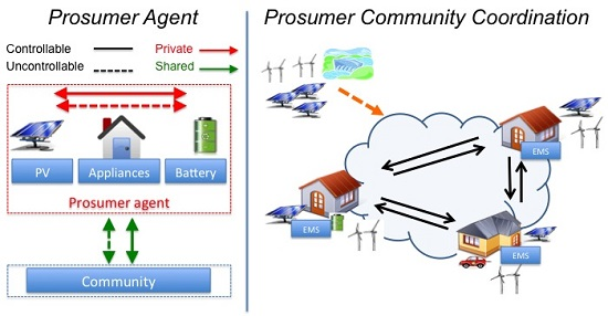
- To allow each agent to manage its QoL and associated power consumption and generation.
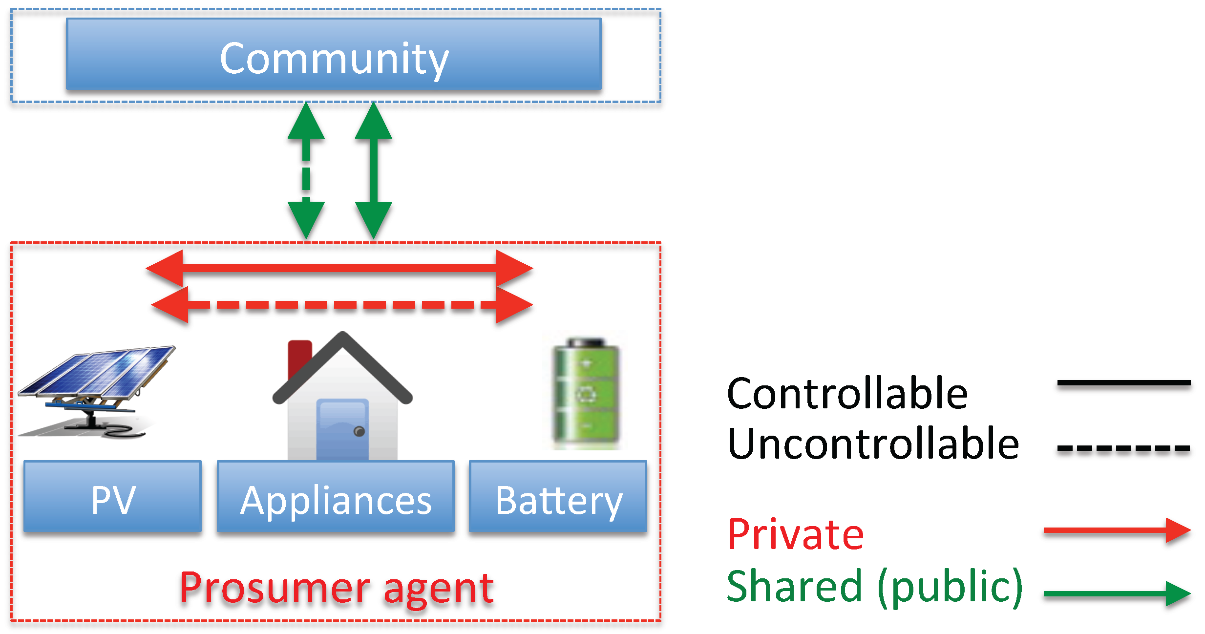
- To allow each user to be a prosumer (i.e., a producer and a consumer).
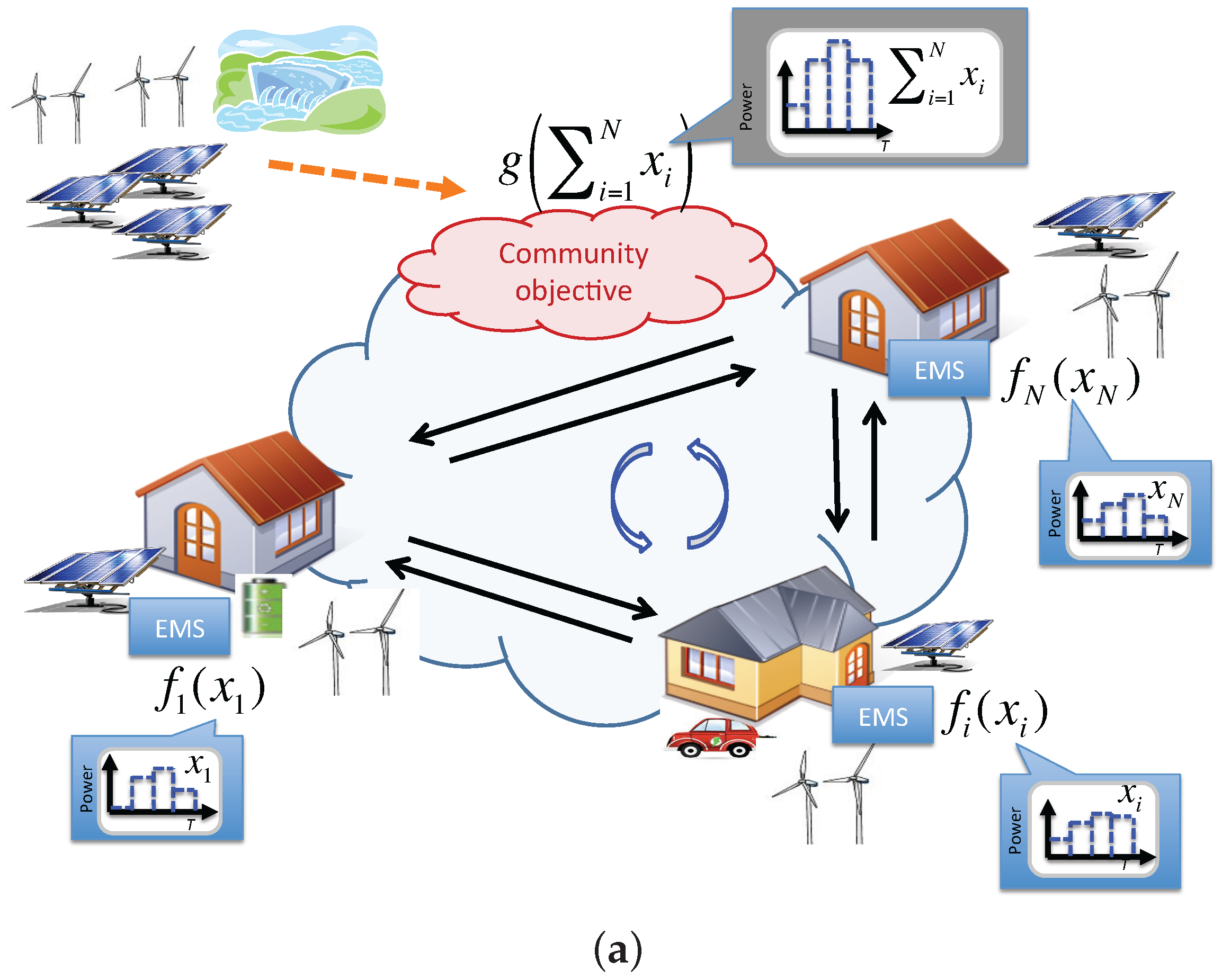
- To allow prosumers to form a community and jointly manage their power usage taking into account a common goal for the community (e.g., reduce cost, increase use of renewables, etc.)
- To achieve full responsiveness in energy management (e.g., that controllable consumption is able to match uncontrollable generation and consumption at all times, instead of just seeking to reduce economical cost, increase stability or respond to external requests).
2.3.1. Day-Ahead Power Consumption Coordination Formulation
2.3.2. Distributed Coordination Protocol
2.4. Illustrative Example
2.4.1. Coordinated Energy Management
2.4.2. Price-Based Demand Response
2.4.3. Results and Discussion
3. Augmented Prosumer Management Model
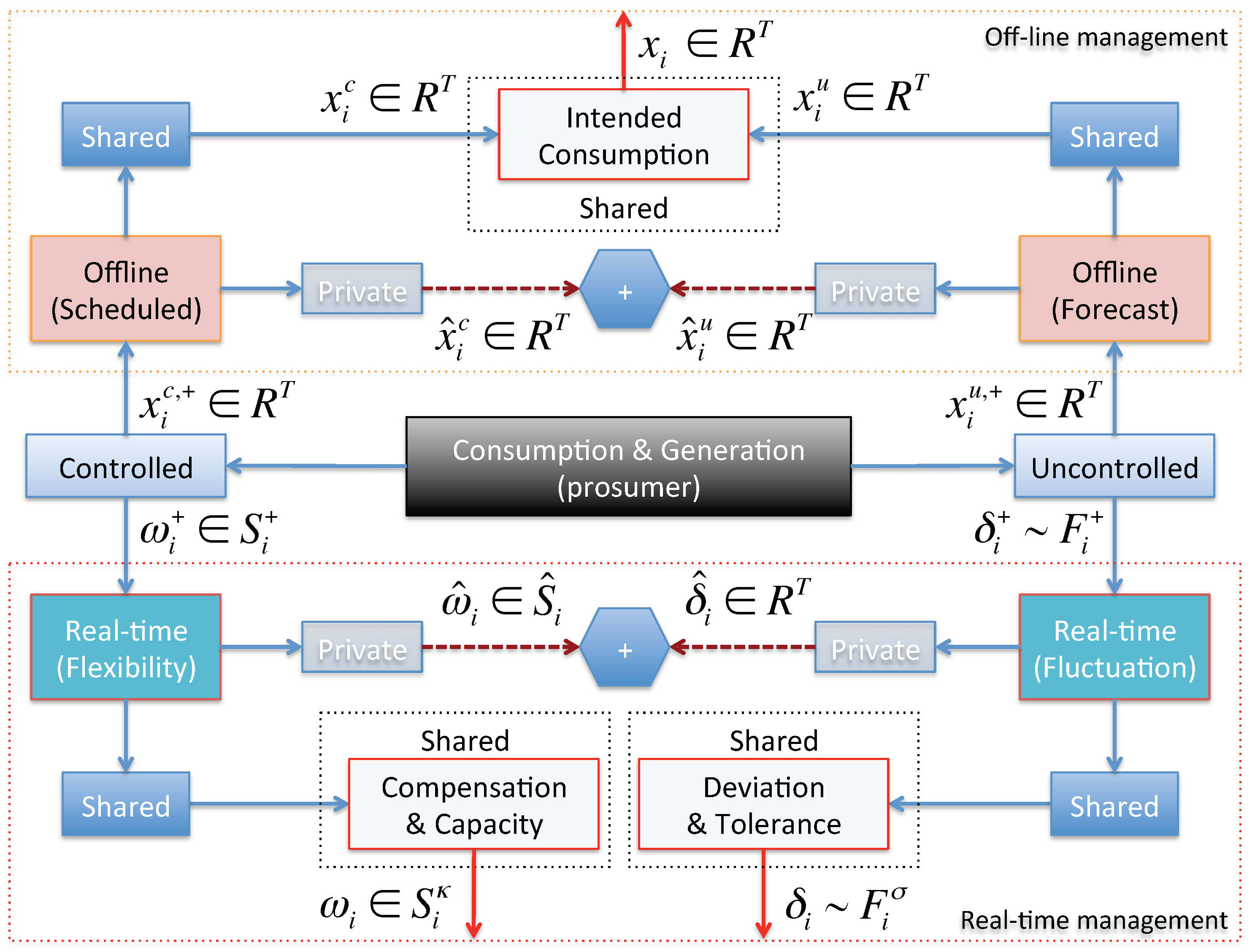
3.1. Augmented Prosumer Model
3.1.1. Power Consumption Decomposition
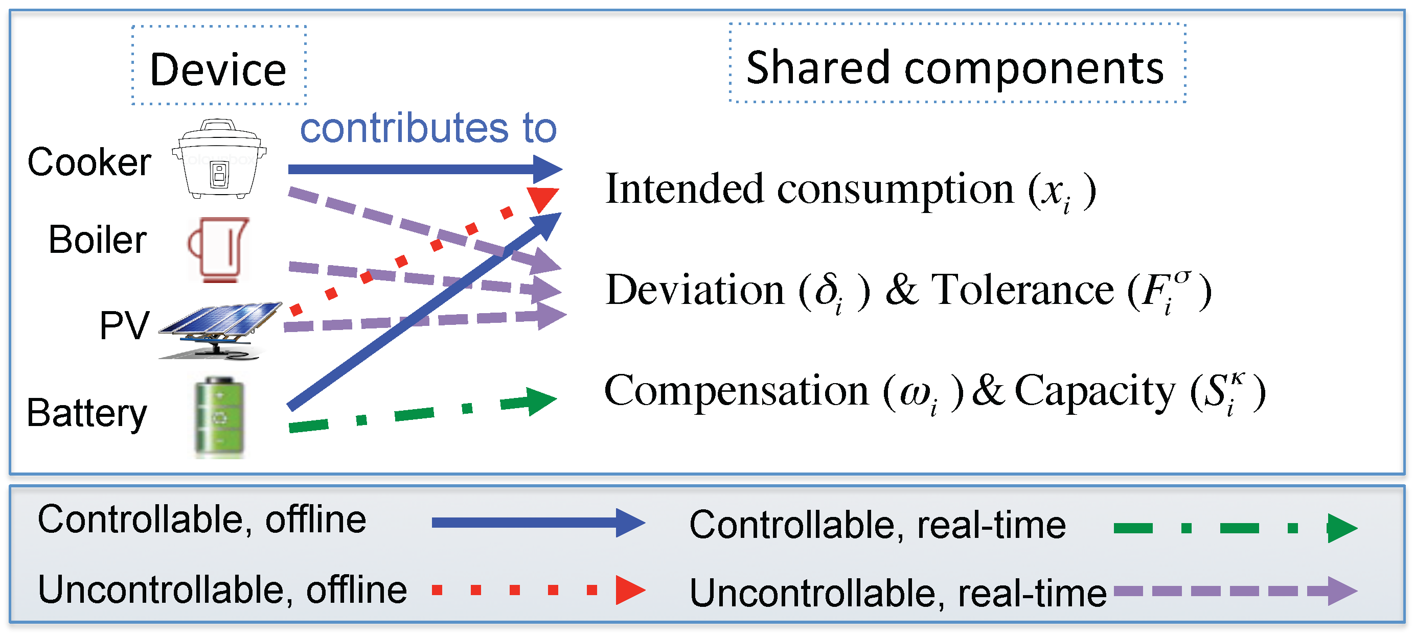
3.2. Augmented Device Model
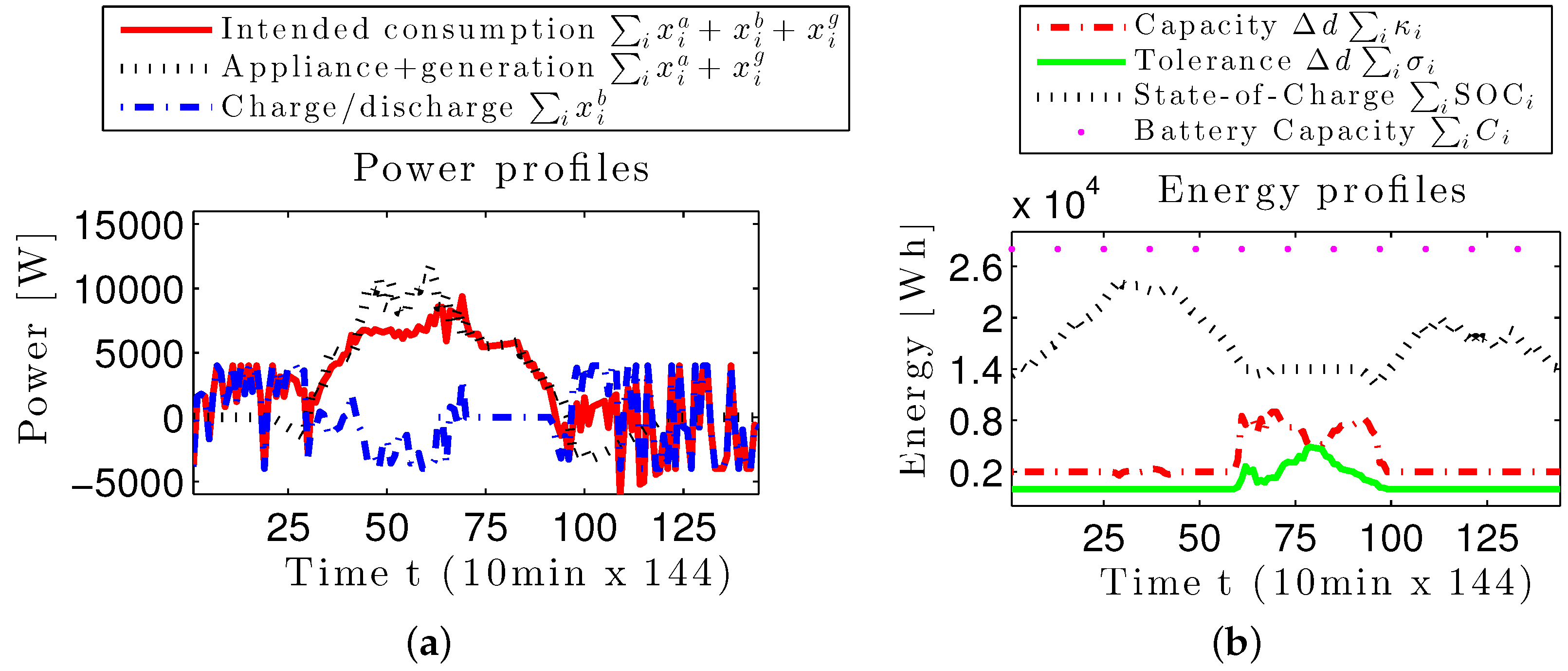
- Intended consumption: , with the intended consumption of device p.
- Compensation (shared and private) and , and capacity (shared and private) and .
- Deviation (shared and private) and , and tolerance (shared and private) and .
4. Augmented Coordinated Energy Management in Prosumer Communities
4.1. Augmented Day-Ahead Coordination
Agent cost
- can measure loss in QoL associated to the device operation mode (due to control signal ),
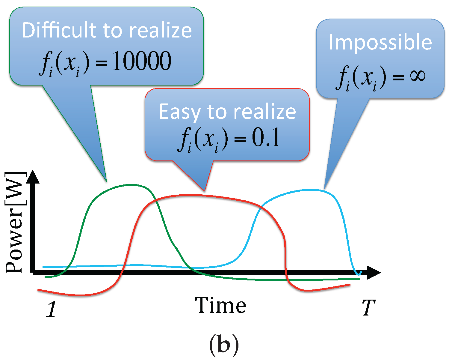
- can represent soft-constraints (e.g. encode achievable profiles due to control ),
- : can measure the agent’s ability to control deviation,
- : economical cost of profile ,
- : penalty of deviating from the power profile plan, and
- : benefit of reserving capacity for the community.
Community cost
- : the cost associated to the intended community aggregated power consumption x, and
- : the degree of capacity relative to tolerance, where ideally, the community capacity should be able manage any tolerance: i.e. .
4.2. Augmented Real-Time Coordination
5. Simulation Results
5.1. Augmented Agent and Coordination Example (Scenario 1)
5.1.1. Device Models
Appliance
Battery
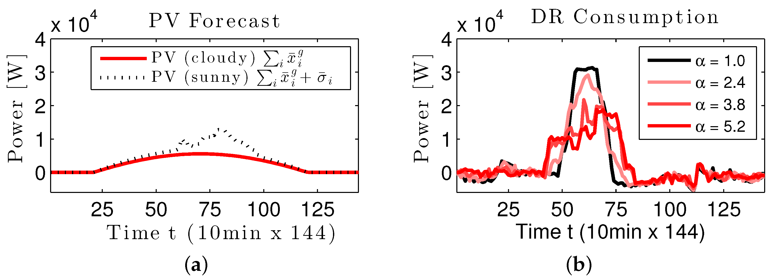
PV Generation
5.1.2. Device Model Aggregation
5.1.3. Cost Functions
5.1.4. Experimental Results
5.2. Augmented Coordination Validation (Scenario 2)
5.2.1. Results
Day-Ahead Augmented Coordination
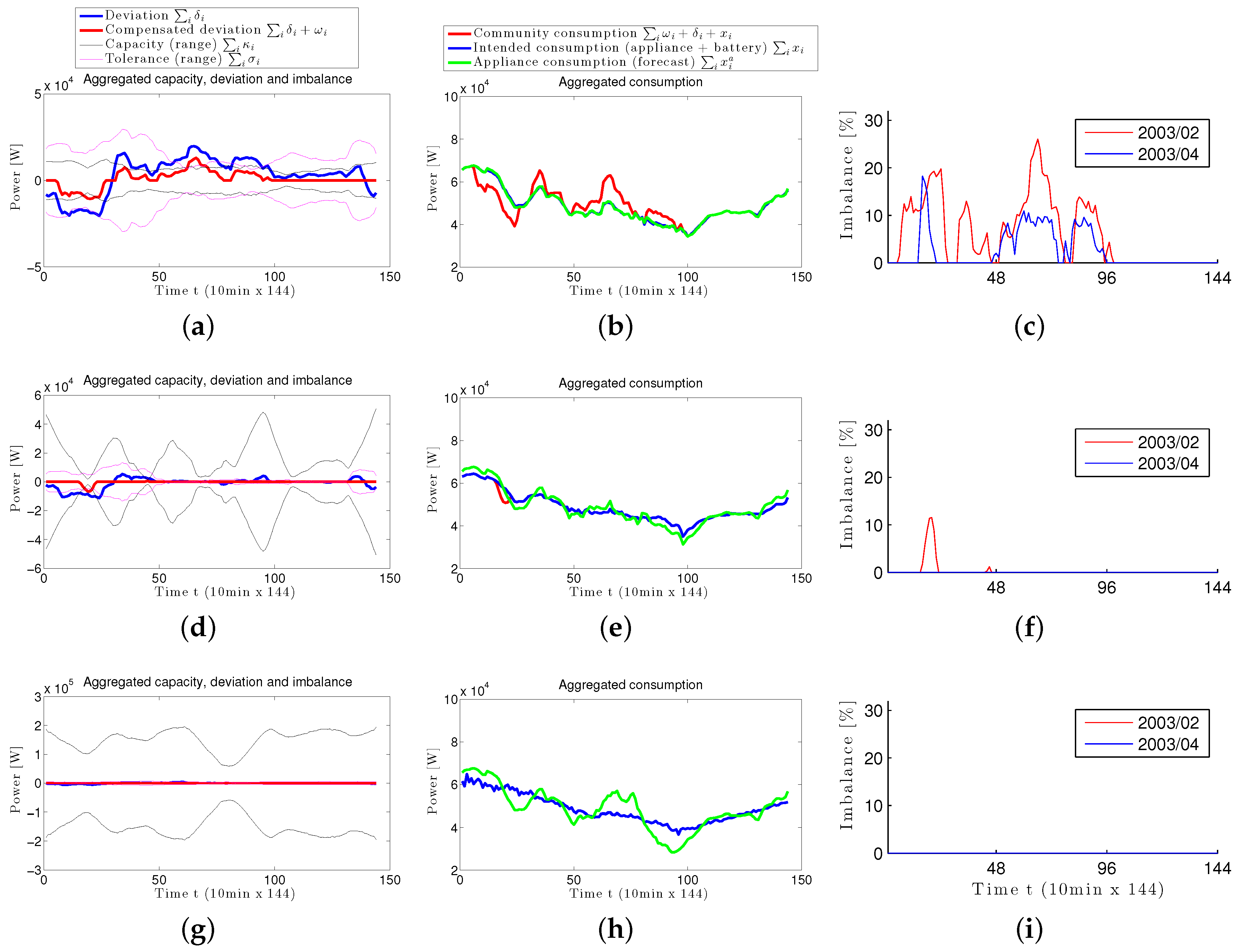
Week-Ahead Augmented Coordination
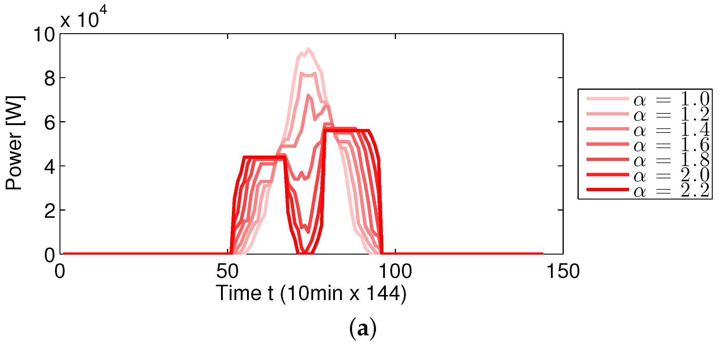
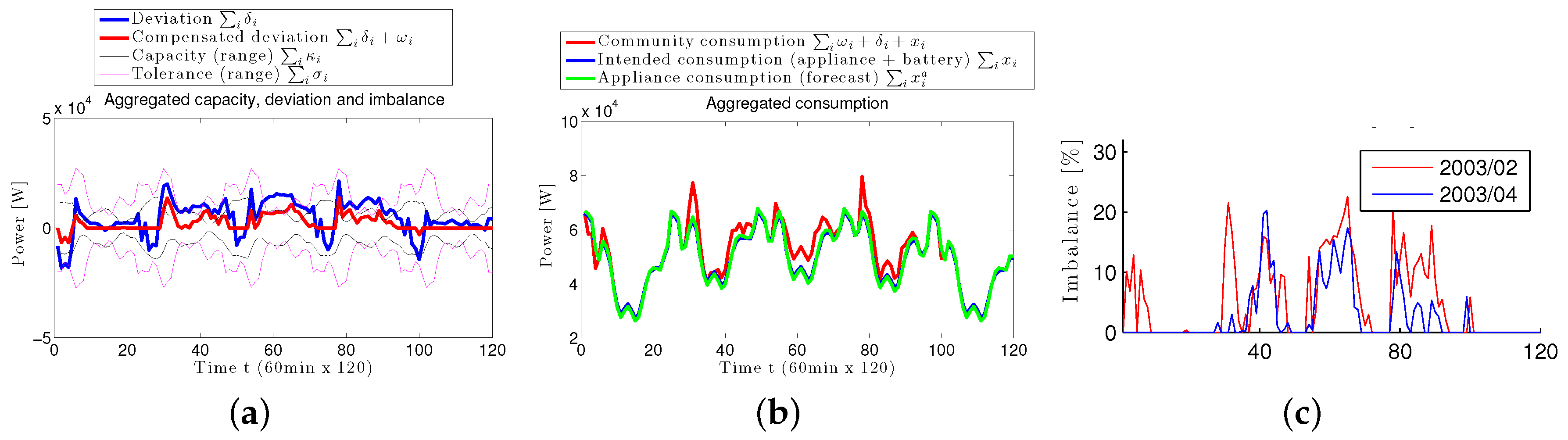
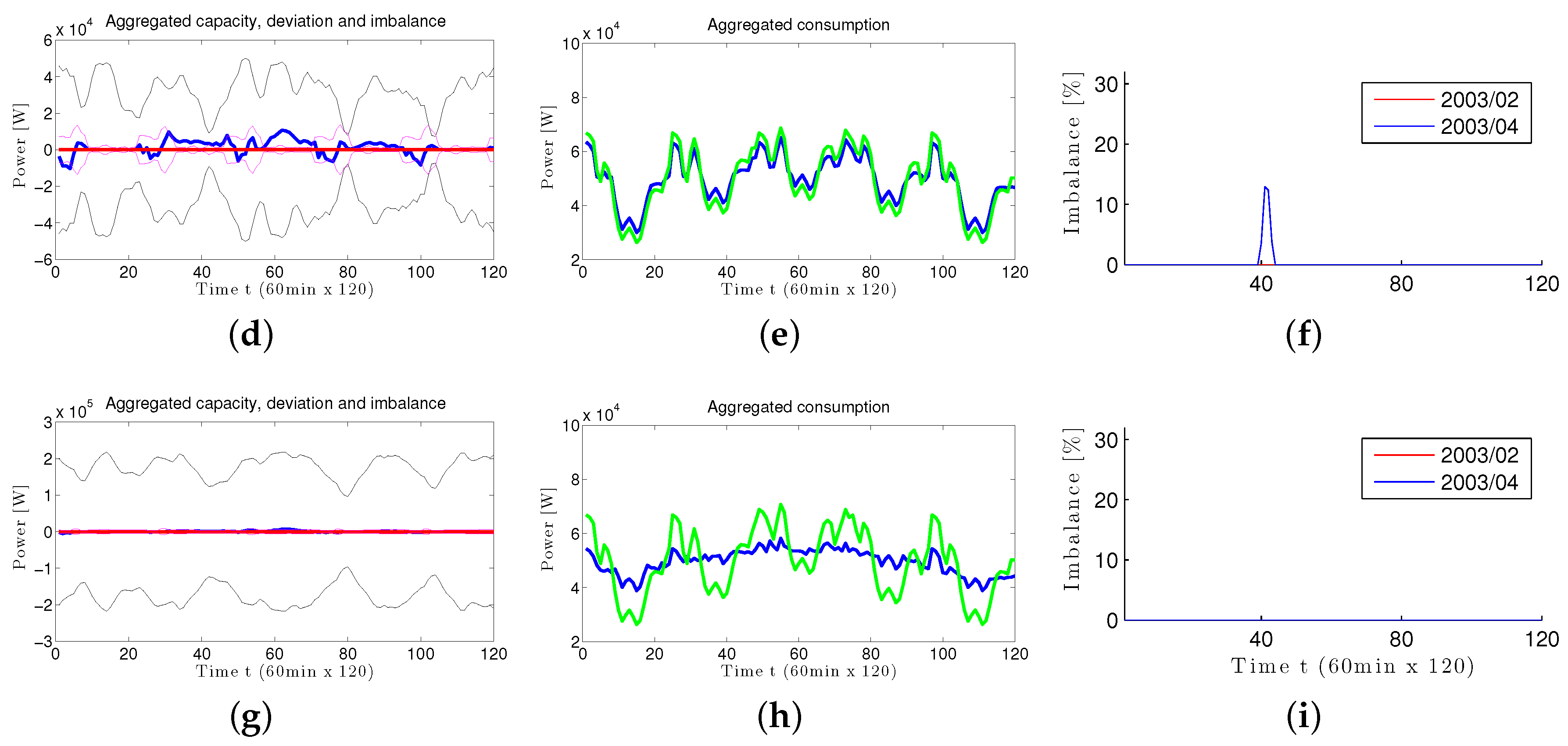
- A tiny battery size per agent () can slightly reduce imbalance but cannot flatten the intended power profile Figure 14a–c.
- A small battery size () (second row) has much more capacity to compensated deviations, slightly flattens the intended power profile, and eliminates almost all imbalance Figure 14d–f.
- A mid battery size () obtains a large community capacity and compensates all deviations, while furthers flattening the intended power consumption profile and generating no imbalance Figure 14g–h.
6. Conclusions
Acknowledgments
Author Contributions
Conflicts of Interest
References
- Stern, D.I. Modeling international trends in energy efficiency. Energy Econ. 2012, 34, 2200–2208. [Google Scholar] [CrossRef]
- Nesheiwat, J.; Cross, J.S. Japan’s post-Fukushima reconstruction: A case study for implementation of sustainable energy technologies. Energy Policy 2013, 60, 509–519. [Google Scholar] [CrossRef]
- Matsuyama, T. i-Energy: Smart demand-side energy management. In Smart Grid Applications and Developments; Mah, D., Hills, P., Li, V.O., Balme, R., Eds.; Green Energy and Technology, Springer: London, UK, 2014; pp. 141–163. [Google Scholar]
- Verschae, R.; Kawashima, H.; Kato, T.; Matsuyama, T. Coordinated energy management for inter-community imbalance minimization. Renew. Energy 2016, 87, 922–935. [Google Scholar] [CrossRef]
- Kawashima, H.; Kato, T.; Matsuyama, T. Distributed mode scheduling for coordinated power balancing. In Proceedings of the 2013 IEEE International Conference on Smart Grid Communications (SmartGridComm), Vancouver, BC, Canada, 21–24 October 2013; pp. 19–24.
- Verschae, R.; Kato, T.; Kawashima, H.; Matsuyama, T. A cooperative distributed protocol for coordinated energy management in prosumer communities. In Proceedings of the Singapore-Japan Joint Workshop on Ambient Intelligence and Sensor Networks (ASN 2015), Singapore, Singapore, 4–5 December 2015.
- Rylatt, R.M.; Snape, J.R.; Allen, P.; Ardestani, B.M.; Boait, P.; Boggasch, E.; Fan, D.; Fletcher, G.; Gammon, R.; Lemon, M.; et al. Exploring smart grid possibilities: A complex systems modelling approach. Smart Grid 2015, 1. [Google Scholar] [CrossRef]
- Ogimoto, K.; Kaizuka, I.; Ueda, Y.; Oozeki, T. A good fit: Japan’s solar power program and prospects for the new power system. IEEE Power Energy Mag. 2013, 11, 65–74. [Google Scholar] [CrossRef]
- Ministry of Economy, Trade and Industry. Report of the Electricity System Reform Expert Subcommittee; METI: Japan, 2013; Available online: http://www.meti.go.jp/english/policy/energy_environment/electricity_system_reform/pdf/201302Report_of_Expert_Subcommittee.pdf (accessed on 7 July 2016).
- Goto, M.; Inoue, T.; Sueyoshi, T. Structural reform of Japanese electric power industry: Separation between generation and transmission & distribution. Energy Policy 2013, 56, 186–200. [Google Scholar]
- Callaway, D.; Hiskens, I. Achieving Controllability of Electric Loads. IEEE Proc. 2011, 99, 184–199. [Google Scholar] [CrossRef]
- Lannoye, E.; Flynn, D.; O’Malley, M. Evaluation of Power System Flexibility. IEEE Trans. Power Syst. 2012, 27, 922–931. [Google Scholar] [CrossRef]
- Sullivan, R.L. Power System Planning; McGraw-Hill Inc.: New York, NY, USA, 1977. [Google Scholar]
- Barbato, A.; Capone, A. Optimization models and methods for demand-side management of residential users: A survey. Energies 2014, 7, 5787–5824. [Google Scholar] [CrossRef]
- Gelazanskas, L.; Gamage, K.A. Demand side management in smart grid: A review and proposals for future direction. Sustain. Cities Soc. 2014, 11, 22–30. [Google Scholar] [CrossRef]
- Mahmood, A.; Javaid, N.; Khan, M.A.; Razzaq, S. An overview of load management techniques in smart grid. Int. J. Energy Res. 2015, 39, 1437–1450. [Google Scholar] [CrossRef]
- O’Connell, N.; Pinson, P.; Madsen, H.; O’Malley, M. Benefits and challenges of electrical demand response: A critical review. Renew. Sustain. Energy Rev. 2014, 39, 686–699. [Google Scholar] [CrossRef]
- Alizadeh, M.; Li, X.; Wang, Z.; Scaglione, A.; Melton, R. Demand-side management in the smart grid: Information processing for the power switch. IEEE Signal Proc. Mag. 2012, 29, 55–67. [Google Scholar] [CrossRef]
- Boait, P.; Ardestani, B.M.; Snape, J.R. Accommodating renewable generation through an aggregator-focused method for inducing demand side response from electricity consumers. IET Renew. Power Gener. 2013, 7, 689–699. [Google Scholar] [CrossRef]
- Roscoe, A.J.; Ault, G. Supporting high penetrations of renewable generation via implementation of real-time electricity pricing and demand response. IET Renew. Power Gener. 2010, 4, 369–382. [Google Scholar] [CrossRef]
- Rastegar, M.; Fotuhi-Firuzabad, M.; Aminifar, F. Load commitment in a smart home. Appl. Energy 2012, 96, 45–54. [Google Scholar] [CrossRef]
- Papadaskalopoulos, D.; Strbac, G. Decentralized, agent-based participation of load appliances in electricity pool markets. In Proceedings of the 21st International Conference on Electricity Distribution, Frankfurt, Germany, 6–9 June 2011.
- Roozbehani, M.; Dahleh, M.A.; Mitter, S.K. Volatility of Power Grids Under Real-Time Pricing. IEEE Trans. Power Syst. 2012, 27, 1926–1940. [Google Scholar] [CrossRef]
- Caron, S.; Kesidis, G. Incentive-based energy consumption scheduling algorithms for the smart grid. In Proceedings of the IEEE International Conference on Smart Grid Communications (SmartGridComm), Gaithersburg, MD, USA, 4–6 October 2010; pp. 391–396.
- Alizadeh, M.; Chang, T.H.; Scaglione, A. Grid integration of distributed renewables through coordinated demand response. In Proceedings of the IEEE 51st Conference on Decision and Control (CDC), Maui, HI, USA, 10–13 December 2012; pp. 3666–3671.
- Chang, T.H.; Alizadeh, M.; Scaglione, A. Real-time power balancing via decentralized coordinated home energy scheduling. IEEE Trans. Smart Grid 2013, 4, 1490–1504. [Google Scholar] [CrossRef]
- Tsai, S.C.; Tseng, Y.H.; Chang, T.H. Communication-efficient distributed demand response: A randomized ADMM approach. IEEE Trans. Smart Grid 2015, PP, 1. [Google Scholar] [CrossRef]
- Hug, G.; Kar, S.; Wu, C. Consensus + Innovations approach for distributed multiagent coordination in a microgrid. IEEE Trans. Smart Grid, 2015, 6, 1893–1903. [Google Scholar] [CrossRef]
- Rahbari-Asr, N.; Ojha, U.; Zhang, Z.; yuen Chow, M. Incremental welfare consensus algorithm for cooperative distributed generation/demand response in smart grid. IEEE Trans. Smart Grid 2014, 5, 2836–2845. [Google Scholar] [CrossRef]
- Del Real, A.; Arce, A.; Bordons, C. An integrated framework for distributed model predictive control of large-scale power networks. IEEE Trans. Ind. Inform. 2014, 10, 197–209. [Google Scholar] [CrossRef]
- Verschae, R.; Kawashima, H.; Kato, T.; Matsuyama, T. A distributed hierarchical architecture for community-based power balancing. In Proceedings of the IEEE International Conference on Smart Grid Communications (SmartGridComm), Venice, Italy, 3–6 November 2014; pp. 169–175.
- Verschae, R.; Kawashima, H.; Kato, T.; Matsuyama, T. A distributed coordination framework for on-line scheduling and power demand balancing of households communities. In Proceedings of the European Control Conference (ECC), Strasbourg, France, 24–27 June 2014; pp. 1655–1662.
- Boyd, S.; Parikh, N.; Chu, E.; Peleato, B.; Eckstein, J. Distributed optimization and statistical learning via the alternating direction method of multipliers. Found. Trends Mach. Learn. 2011, 3, 1–122. [Google Scholar] [CrossRef]
- Boyd, S.; Vandenberghe, L. Convex Optimization; Cambridge University Press: Cambridge, UK, 2004. [Google Scholar]
- Combettes, P.; Pesquet, J.C. Proximal splitting methods in signal processing. In Fixed-Point Algorithms for Inverse Problems in Science and Engineering; Bauschke, H.H., Burachik, R.S., Combettes, P.L., Elser, V., Luke, D.R., Wolkowicz, H., Eds.; Springer Optimization and Its Applications, Springer: New York, NY, USA, 2011; pp. 185–212. [Google Scholar]
- Parikh, N.; Boyd, S. Proximal algorithms. Found. Trends Optim. 2014, 1, 127–239. [Google Scholar] [CrossRef]


© 2016 by the authors; licensee MDPI, Basel, Switzerland. This article is an open access article distributed under the terms and conditions of the Creative Commons Attribution (CC-BY) license (http://creativecommons.org/licenses/by/4.0/).
Share and Cite
Verschae, R.; Kato, T.; Matsuyama, T. Energy Management in Prosumer Communities: A Coordinated Approach. Energies 2016, 9, 562. https://doi.org/10.3390/en9070562
Verschae R, Kato T, Matsuyama T. Energy Management in Prosumer Communities: A Coordinated Approach. Energies. 2016; 9(7):562. https://doi.org/10.3390/en9070562
Chicago/Turabian StyleVerschae, Rodrigo, Takekazu Kato, and Takashi Matsuyama. 2016. "Energy Management in Prosumer Communities: A Coordinated Approach" Energies 9, no. 7: 562. https://doi.org/10.3390/en9070562
APA StyleVerschae, R., Kato, T., & Matsuyama, T. (2016). Energy Management in Prosumer Communities: A Coordinated Approach. Energies, 9(7), 562. https://doi.org/10.3390/en9070562