
Comparative Life Cycle Cost Analysis of Hardening Options for Critical Loads

 , ,
, ,
Abstract
:
1. Introduction
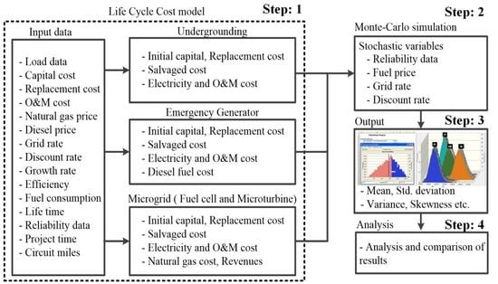
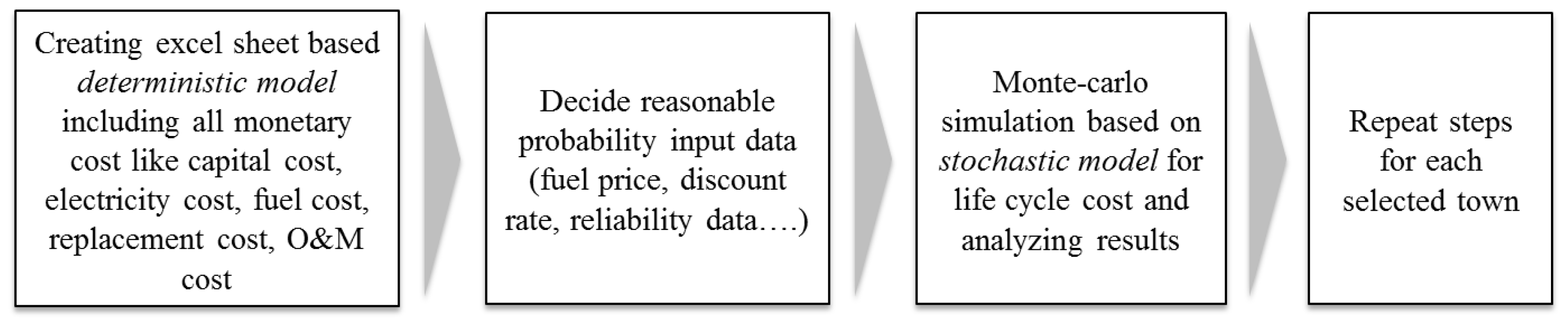
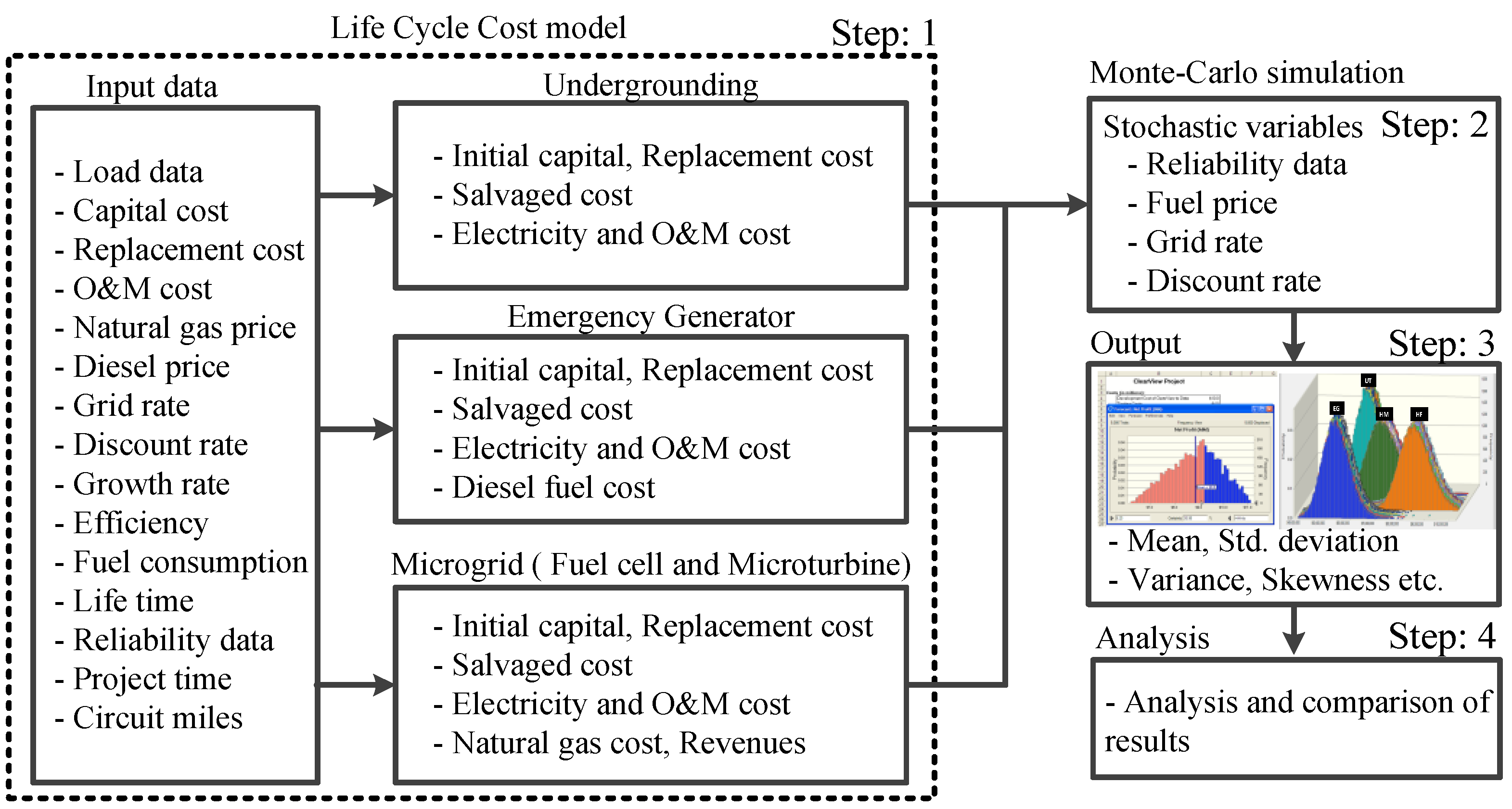
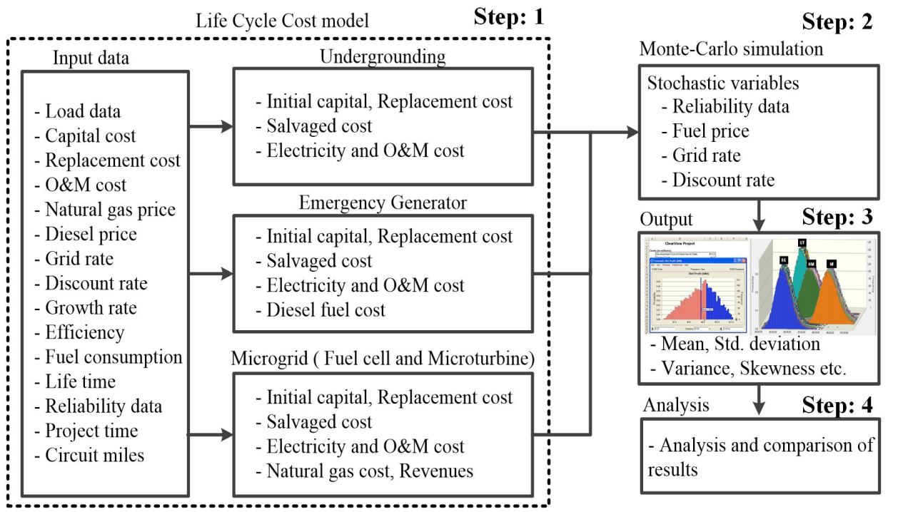
2. Methodology
- only electric loads are considered;
- microgrid distributed generation sources are running all of the time; and
- all generators are assumed to have a single interconnection point.
3. Formulas for Estimating Life Cycle Cost
3.1. Net Present Cost
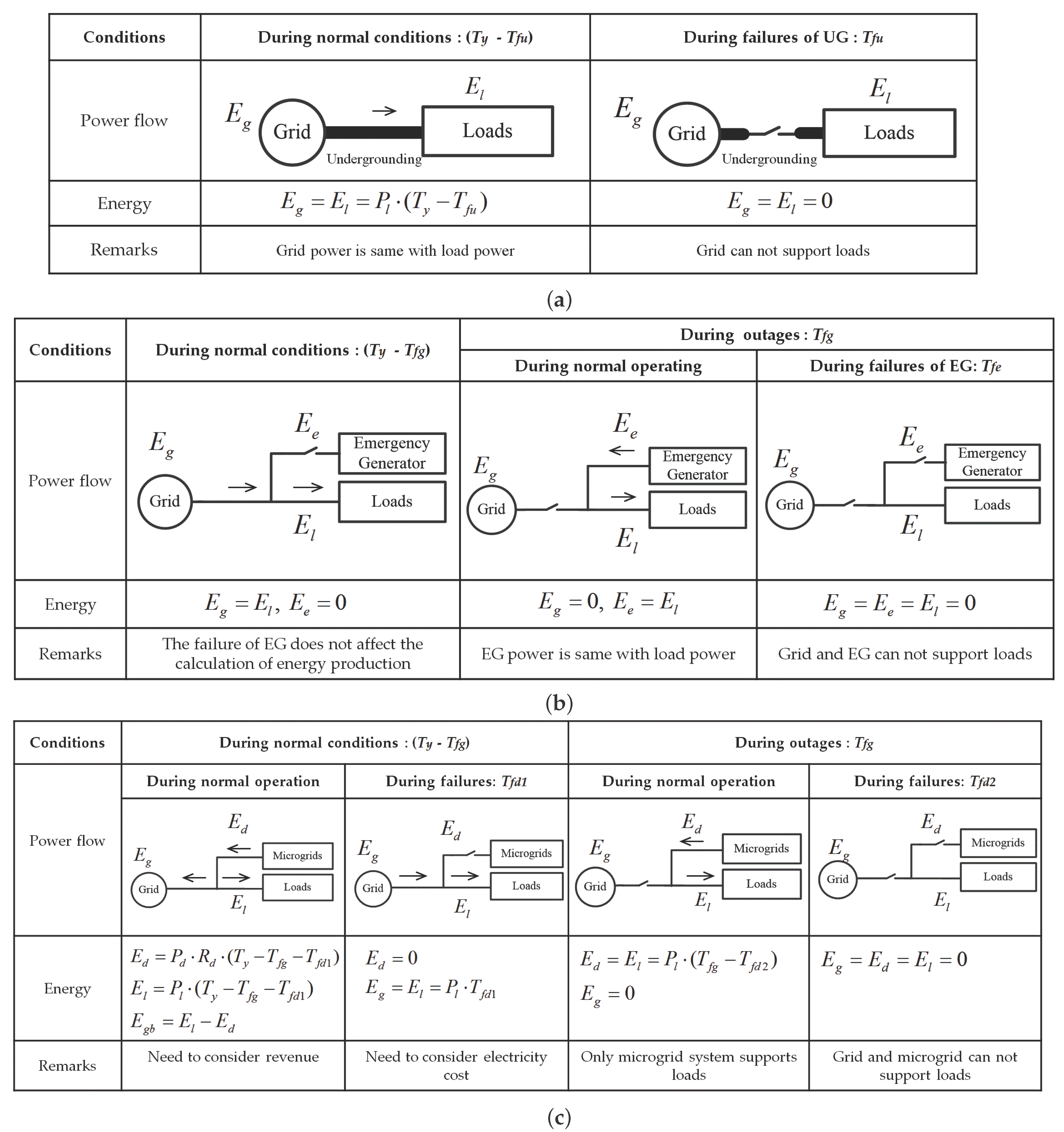
3.2. Energy Production
3.2.1. Undergrounding
3.2.2. Emergency Generator
3.2.3. Microgrid
3.3. Annual Operating Cost
3.3.1. Undergrounding
3.3.2. Emergency Generator
3.3.3. Microgrid
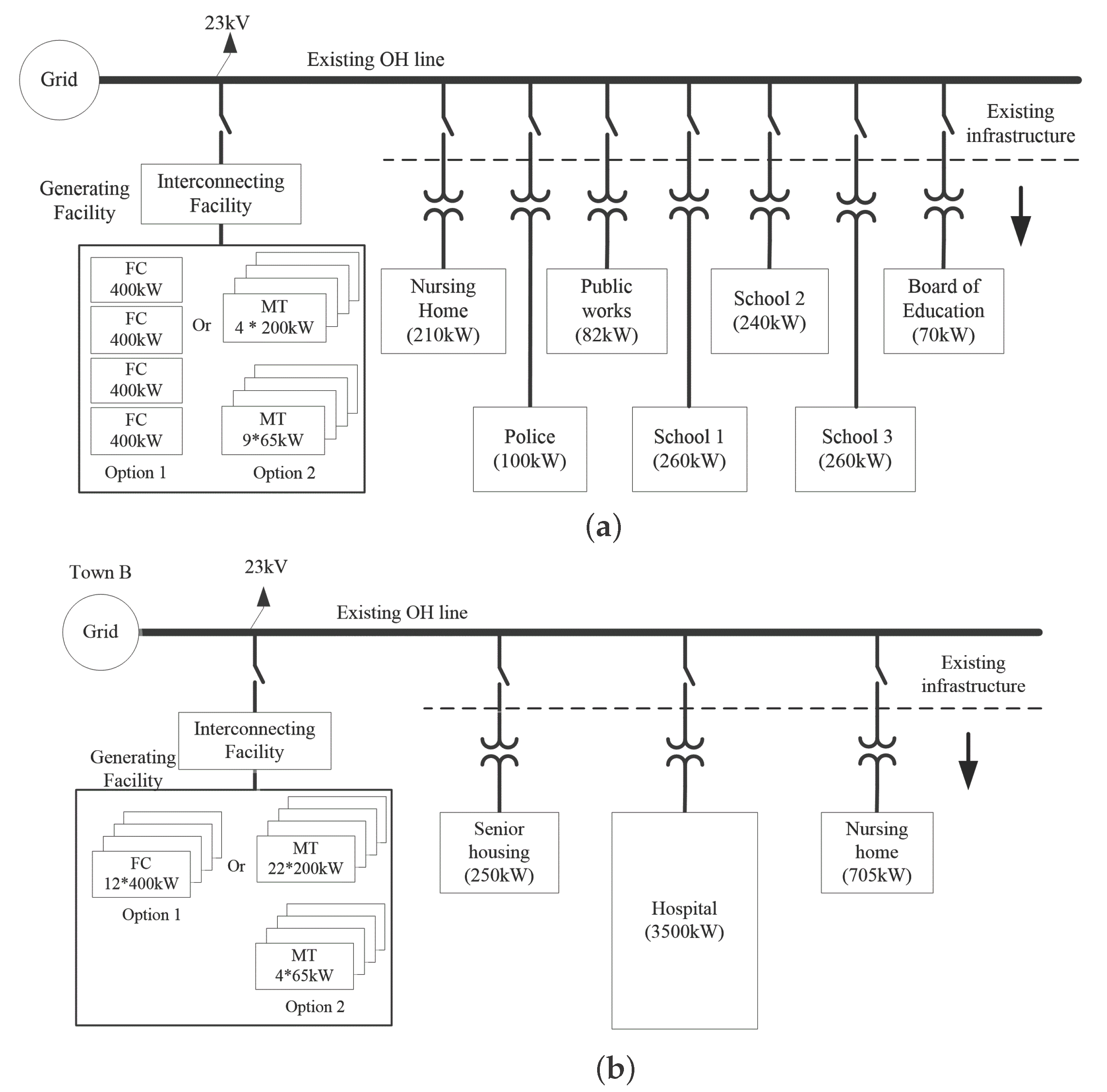
4. Case Study
4.1. General Input Data
4.2. Probabilistic Input Data
4.2.1. Reliability Data of Hardening Options
4.2.2. Discount Rate and Growth Rate
4.2.3. Grid Rate
4.2.4. Natural Gas Price
4.2.5. Diesel Price
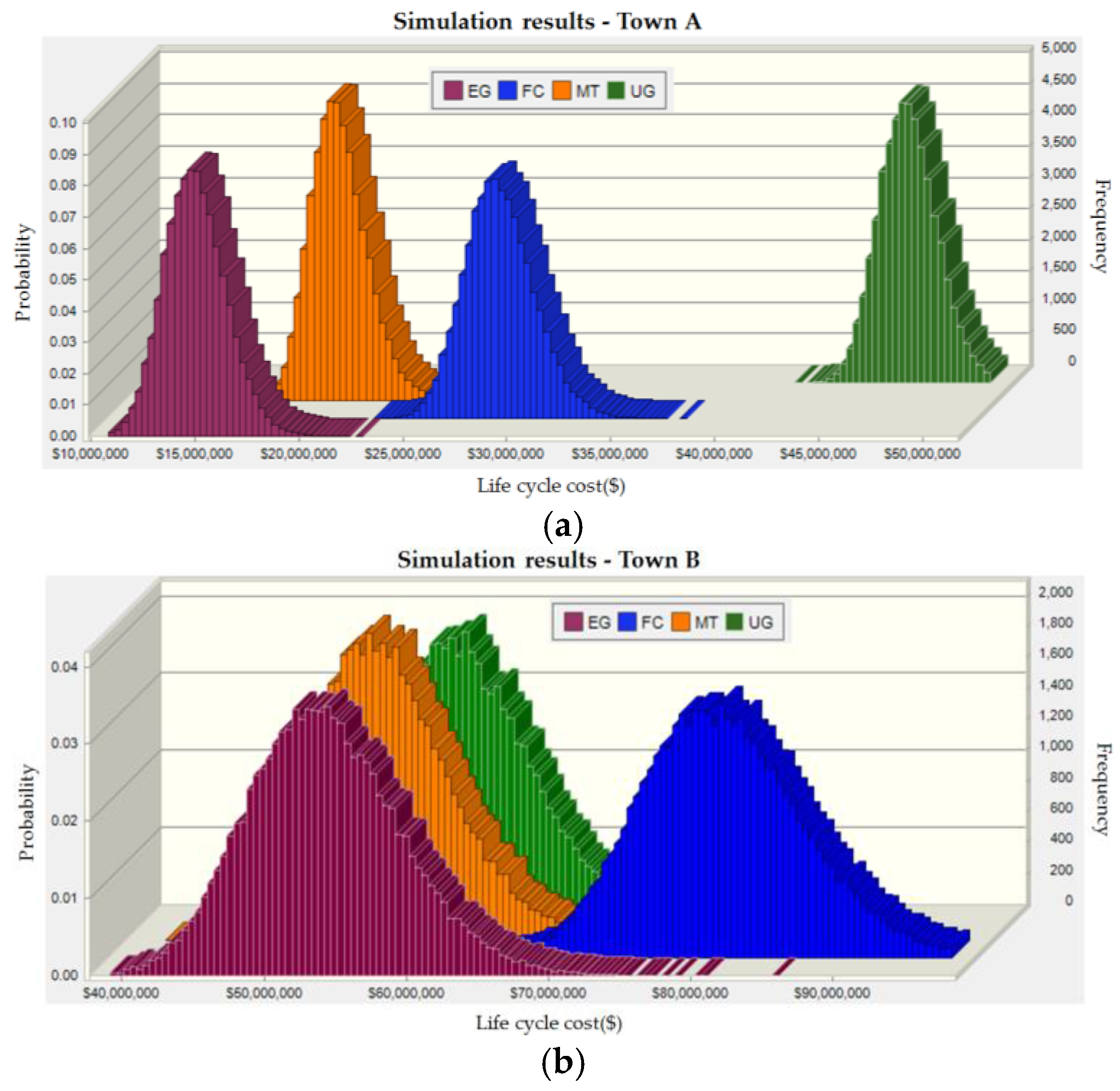
4.3. Monte Carlo Simulation Results
5. Conclusions
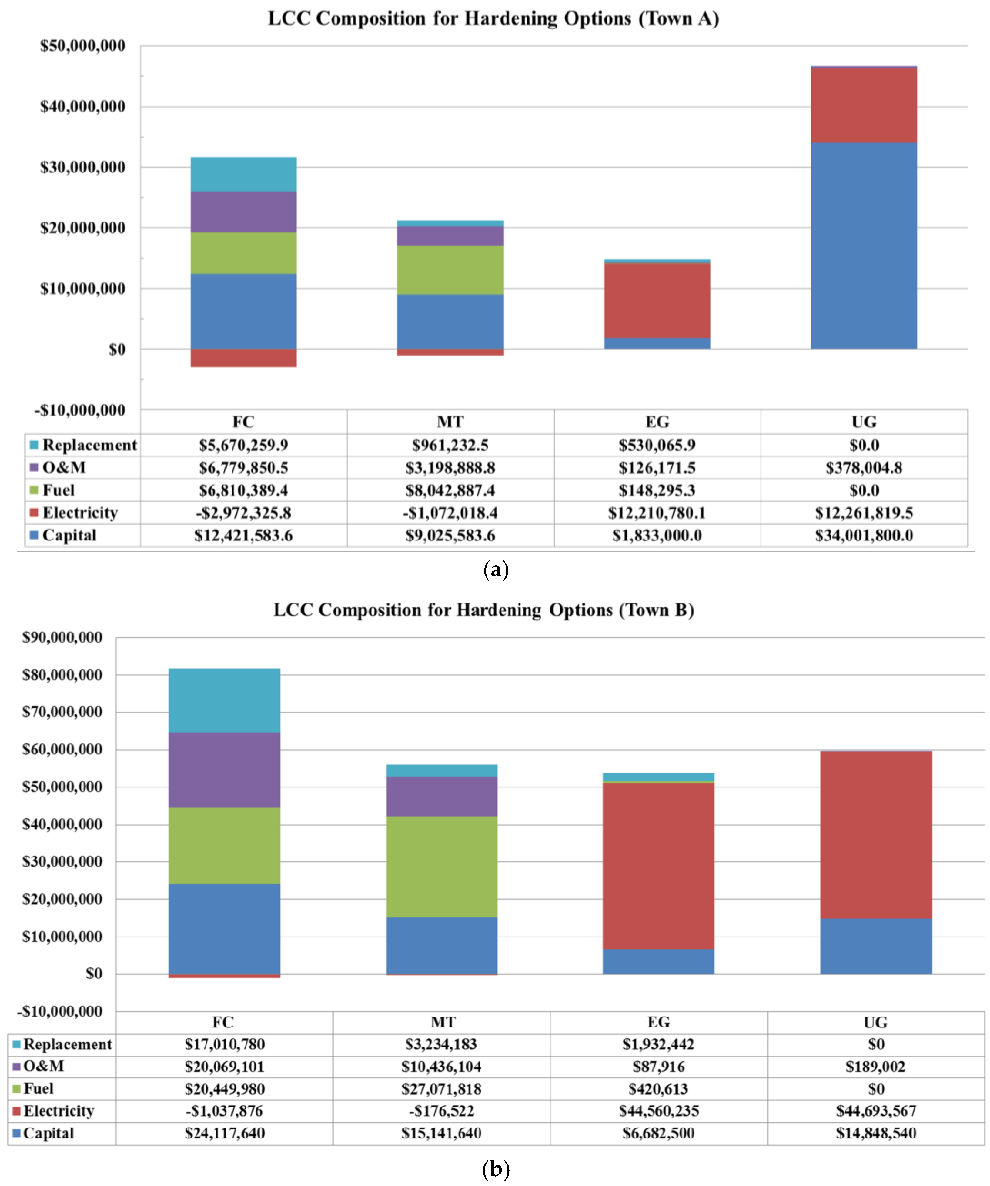
- EG have a lower LCC for power system hardening compared to other hardening options due to low initial capital cost. Additionally, the installation and maintenance are simple and easy. However, if the power outage happens more frequently due to extreme weather events, the operating cost of EGs, like the fuel and O&M costs, tend to significantly increase and, thus, EG as an option will be less attractive in hardening a power system.
- UG can be an alternative solution since UG tends to have low operating costs, such as low O&M and electricity generation costs. Additionally, it has a longer lifetime compared to other options. However, UG tends to have a high initial capital cost and longer construction time, which makes UG less attractive. If the circuit miles of UG are short and the initial capital costs are relatively low, UG can be a better candidate as a hardening option.
- FC systems generally have high initial and replacement costs in spite of high efficiency and environmentally friendly operation. Additionally, its operating cost depends highly on the fuel and O&M costs. FC systems can become a better option as a sustainable energy source if their technology is enhanced and their capital, replacement, and O&M costs are reduced in the future.
- MT systems can be an alternative solution among many existing distributed generation systems. Their capital and operating costs reach an acceptable level compared to other distributed sources, such as PV, wind turbine, and FC.
Acknowledgments
Author Contributions
Conflicts of Interest
Nomenclature
| x | Subscripts to represent: |
| g: grid; | |
| u: undergrounding; | |
| e: emergency generator; | |
| d: microgrid; | |
| l: critical loads; | |
| oh: overhead-line system | |
| Yp | Project time (year) |
| Ty | Total hours for one year (hour) |
| Tfx | Interruption hours by failures of “x” (hour/year) |
| Trx | Running-time of “x” (years) |
| Tx | Life-time of “x”(years) |
| Ex | Annual power from “x” (kWh/year) |
| Egb | Annual power back to grid (kWh/year) |
| Px | Rated power of “x” (years) |
| Rd | Averaged annual operation ratio of microgrids |
| ηx | Efficiency of generator unit “x” (%) |
| rnet | Annual net discount rate (%) |
| rd | Annual discount rate (%) |
| rg | Annual grow rate (%) |
| Fds | Diesel consumption coefficient (L/kWh) |
| Fng | Natural gas consumption coefficient (m3/kWh) |
| Lug | Circuit miles of undergrounding line (mile) |
| Loh | Circuit miles of overhead line (mile) |
| CNPC | Total net present cost ($) |
| Cic | total initial capital cost ($) |
| Csvg | Salvaged cost of power generator unit ($) |
| Coa | Annual total operating cost ($/year) |
| Cel | Annual net electricity cost ($/year) |
| Crv | Annual revenue ($/year) |
| Cf | Annual fuel cost ($/year) |
| Cre | Annual replacement cost ($/year) |
| COM | Annual O&M cost ($/year) |
| Cbg | Buying rate from grid ($/kWh) |
| Csg | Selling rate to grid ($/kWh) |
| Cng | Natural gas price ($/m3) |
| Cds | Diesel price ($/L) |
| CxOM | O&M cost of “x” generator unit ($/kWh, $/mile) |
| CxREP | Replacement cost of “x”generator unit ($) |
References
- McGee, J.; Skif, J.; Carozza, P.; Edelstein, T.; Hoffman, L.; Jackson, S.; McGrath, R.; Osten, C. Report of the Two Storm Panel; January 2012. Available online: http://portal.ct.gov/Departments_and_Agencies/Office_of_the_Governor/Learn_More/Working_Groups/two_storm_panel_final_report/ (accessed on 14 July 2016).
- Maney, C.T. Benefits of urban underground power delivery. IEEE Technol. Soc. Mag. 1996, 15, 12–22. [Google Scholar] [CrossRef]
- Castenschiold, R. Solutions to industrial and commercial needs using multiple utility services and emergency generator sets. IEEE Trans. Ind. Appl. 1974, IA-10, 205–208. [Google Scholar] [CrossRef]
- Venkataramanan, G.; Marnay, C. A larger role for microgrids. IEEE Power Energy Mag. 2008, 6, 78–82. [Google Scholar] [CrossRef]
- Woodward, D.G. Life cycle costing—Theory, information acquisition and application. Int. J. Proj. Manag. 1997, 15, 335–344. [Google Scholar] [CrossRef]
- Curry, E.E. STEP: A tool for estimating avionics life cycle costs. IEEE Aerosp. Electron. Syst. Mag. 1989, 4, 30–32. [Google Scholar] [CrossRef]
- Schoenung, S.M.; Hassenzahl, W.V. Long- vs. Short-Term Energy Storage Technologies Analysis. A Life-Cycle Cost Study. A Study for the DOE Energy Storage Systems Program; Sandia National Laboratories: Albuquerque, NM, USA, 2003. [Google Scholar]
- Roth, I.F.; Ambs, L.L. Incorporating externalities into a full cost approach to electric power generation life-cycle costing. Energy 2004, 29, 2125–2144. [Google Scholar] [CrossRef]
- Lambert, T.; Gilman, P.; Lilienthal, P. Micropower system modeling with HOMER. In Integration of Alternative Sources of Energy; Farret, F.A., Simões, M.G., Eds.; Wiley: Hoboken, NJ, USA, 2006; pp. 379–418. [Google Scholar]
- Nelson, D.B.; Nehrir, M.H.; Gerez, V. Economic evaluation of grid-connected fuel-cell systems. IEEE Trans. Energy Convers. 2005, 20, 452–458. [Google Scholar] [CrossRef]
- Wies, R.W.; Johnson, R.A.; Agrawal, A.N.; Chubb, T.J. Simulink model for economic analysis and environmental impacts of a PV with diesel-battery system for remote villages. IEEE Trans. Power Syst. 2005, 20, 692–700. [Google Scholar] [CrossRef]
- Brown, R.E. Hurricane hardening efforts in Florida. In Proceedings of the IEEE Power and Energy Society General Meeting—Conversion and Delivery of Electrical Energy in the 21st Century, Pittsburgh, PA, USA, 20–24 July 2008; pp. 1–7.
- Holt, L.; Kury, T.K. Florida’s storm hardening effort: A new paradigm for state utility regulators. Electr. J. 2011, 24, 62–71. [Google Scholar] [CrossRef]
- Boggess, J.M.; Becker, G.W.; Mitchell, M.K. Storm & flood hardening of electrical substations. In Proceedings of the IEEE PES T & D Conference and Exposition, Chicago, IL, USA, 14–17 April 2014.
- Bernal-Agustín, J.L.; Dufo-Lopez, R. Simulation and optimization of stand-alone hybrid renewable energy systems. Renew. Sustain. Energy Rev. 2009, 13, 2111–2118. [Google Scholar] [CrossRef]
- Park, S.M.; Park, S.Y.; Zhang, P.; Luh, P.; Rakotomavo, M.T.J.; Serna, C. Comparative life cycle cost analysis of hardening options for critical loads. In Proceedings of the IEEE PES Innovative Smart Grid Technologies Conference (ISGT), Washington, DC, USA, 19–22 February 2014.
- Darrow, K.; Tidball, R.; Wang, J.; Hampson, A. Catalogue of CHP Technologies; U.S. Environmental Protection Agency: Washington, DC, USA, 2008.
- Energy and Environmental Analysis. Technology Characterization: Reciprocating Engines; U.S. Environmental Protection Agency: Washington, DC, USA, 2008.
- Energy Information Administration. Annual Energy Outlook 2012; U.S. Energy Information Administration: Washington, DC, USA, 2012.
- Doosan Fuel Cell. America. Purecell Model 400 Datasheet; Doosan Fuel Cell America: South Windsor, CT, USA, 2014. [Google Scholar]
- Caterpillar. Diesel Generator Set: STANDBY 500ekW, 625kVA; Caterpillar: Peoria, IL, USA, 2013. [Google Scholar]
- The Feasibility of Placing Electric Distribution Facilities Underground; North Carolina Public Utilities Commission: Raleigh, NC, USA, 2003.
- Li, G.; Zhang, P.; Luh, P.B.; Li, W. Risk analysis for distribution systems in the northeast U.S. under wind storms. IEEE Trans. Power Syst. 2014, 29, 889–898. [Google Scholar] [CrossRef]
- Department of Public Utility Control. Application of the Connecticut Light & Power Company to Amend Its Rate Schedules; State of Connecticut: Hartford, CT, USA, 2010.
- Darman, R. Guideline and Discount Rates for Benefit-Cost Analysis of Federal Programs; Circular No. A-94 Revised; Office of Management and Budget: Washington, DC, USA, 1992.
- Black, F.; Scholes, M. The pricing of options and corporate liabilities. J. Political Econ. 1973, 81, 637–654. [Google Scholar] [CrossRef]
- CME Group. Henry Hub Natural Gas Futures Quotes. Available online: http://www.cmegroup.com/trading/energy/natural-gas/natural-gas.html (accessed on 14 July 2016).
- CME Group. NY Harbor ULSD Futures Quotes. Available online: http://www.cmegroup.com/trading/energy/refined-products/heating-oil.html (accessed on 14 July 2016).


| Data | Option | Value | Remarks |
|---|---|---|---|
| Project Time | - | 40 years | - |
| Capital cost; Town A [17,18,19] | UG | $34,001,800 | Circuit miles: 8.8 |
| EG | $1200/kW | Rated power: 1222 kW | |
| MT | $2400/kW | Included tax credit, rated power: 1385 kW | |
| FC | $4200/kW | Included tax credit, rated power: 1600 kW | |
| Capital cost; Town B [17,18,19] | UG | $14,848,540 | Circuit miles: 4.4 |
| EG | $1200/kW | Rated power: 4455 kW | |
| MT | $2400/kW | Included tax credit, rated power: 4660 kW | |
| FC | $4200/kW | Included tax credit, rated power: 4800 kW | |
| Replacement cost ratio | EG | 1.0 | System replacment: 1.0 |
| MT | 1.0 | System replacment: 1.0 | |
| FC | 0.8 and 1.0 | Stack: 0.8, System: 1.0 | |
| Efficiency [17,20] | EG | N/A | Fuel consumption curve includes efficiency data |
| MT | 34% | - | |
| FC | 43.5%–48% | Stack aging degradation: 0.5%/year for 10 years | |
| Fuel consumption curve | EG | 0.277 L/kWh [21] | Including EG efficiency |
| MT | 0.0941 m3/kWh | - | |
| FC | 0.0941 m3/kWh | - | |
| Operating ratio (annual) | MT | 0.96 | - |
| FC | 0.95 | - | |
| O&M cost [17,22] | UG | $4052/mile | Over-head QandM: $917/mile |
| EG | $0.015/kWh | - | |
| MT | $0.0185/kWh | - | |
| FC | $0.035/kWh | - | |
| Life time | UG | 40 years | - |
| EG,MT,FC | 20 years | FC Stack: 10 years [20] |
| Do-Nothing (Tfg) | UG | EG | MT | FC | |||||
|---|---|---|---|---|---|---|---|---|---|
| SAIDI (h/year) | Pro. | SAIDI (h/year) | Pro. | SAIDI (h/year) | Pro. | SAIDI (h/year) | Pro. | SAIDI (h/year) | Pro. |
| 47.02 | 0.975029 | 10.20 | 0.999924 | 1.90 | 0.997043 | 4.17 | 0.999802 | 6.43 | 0.999869 |
| 141.06 | 0.000517 | 30.61 | 0.000010 | 5.71 | 0.001194 | 12.51 | 0.000031 | 19.28 | 0.000021 |
| 235.10 | 0.000769 | 51.02 | 0.000007 | 9.51 | 0.000717 | 20.86 | 0.000028 | 32.14 | 0.000015 |
| 329.14 | 0.001704 | 71.42 | 0.000008 | 13.32 | 0.000425 | 29.20 | 0.000023 | 44.99 | 0.000011 |
| 423.18 | 0.003484 | 91.83 | 0.000006 | 17.13 | 0.000264 | 37.54 | 0.000026 | 57.85 | 0.000010 |
| 517.23 | 0.005039 | 112.24 | 0.000004 | 20.93 | 0.000175 | 45.89 | 0.000020 | 70.70 | 0.000010 |
| 611.27 | 0.004941 | 132.64 | 0.000008 | 24.74 | 0.000103 | 54.23 | 0.000011 | 83.56 | 0.000010 |
| 705.31 | 0.003881 | 153.05 | 0.000003 | 28.54 | 0.000046 | 62.57 | 0.000015 | 96.42 | 0.000012 |
| 799.35 | 0.002390 | 173.46 | 0.000001 | 32.35 | 0.000015 | 70.92 | 0.000006 | 109.27 | 0.000007 |
| 893.39 | 0.001235 | 193.86 | 0.000005 | 36.16 | 0.000009 | 79.26 | 0.000011 | 122.13 | 0.000004 |
| 987.43 | 0.000509 | 214.27 | 0.000007 | 39.96 | 0.000003 | 87.60 | 0.000005 | 134.98 | 0.000005 |
| 1081.47 | 0.000245 | 234.68 | 0.000003 | 43.77 | 0.000001 | 95.95 | 0.000005 | 147.84 | 0.000004 |
| 1175.51 | 0.000140 | 255.08 | 0.000004 | 47.57 | 0.000001 | 104.29 | 0.000004 | 160.69 | 0.000003 |
| 1269.55 | 0.000043 | 275.49 | 0.000003 | 51.38 | 0.000001 | 112.63 | 0.000004 | 173.55 | 0.000004 |
| 1363.60 | 0.000029 | 295.90 | 0.000001 | 55.18 | 0.000000 | 120.98 | 0.000002 | 186.40 | 0.000004 |
| 1457.64 | 0.000021 | 316.30 | 0.000002 | 58.99 | 0.000002 | 129.32 | 0.000002 | 199.26 | 0.000001 |
| 1551.68 | 0.000012 | 336.71 | 0.000000 | 62.80 | 0.000000 | 137.66 | 0.000001 | 212.11 | 0.000004 |
| 1645.72 | 0.000006 | 357.12 | 0.000001 | 66.60 | 0.000000 | 146.01 | 0.000001 | 224.97 | 0.000000 |
| 1739.76 | 0.000003 | 377.52 | 0.000001 | 70.41 | 0.000000 | 154.35 | 0.000002 | 237.83 | 0.000002 |
| 1833.80 | 0.000003 | 397.93 | 0.000002 | 74.21 | 0.000001 | 162.69 | 0.000001 | 250.68 | 0.000004 |
| Do-Nothing (Tfg) | UG | EG | MT | FC | |||||
|---|---|---|---|---|---|---|---|---|---|
| SAIDI (h/year) | Pro. | SAIDI (h/year) | Pro. | SAIDI (h/year) | Pro. | SAIDI (h/year) | Pro. | SAIDI (h/year) | Pro. |
| 44.14 | 0.975454 | 16.53 | 0.999935 | 2.22 | 0.999016 | 3.98 | 0.999876 | 4.69 | 0.999934 |
| 132.42 | 0.002403 | 49.58 | 0.000012 | 6.65 | 0.000233 | 11.94 | 0.000029 | 14.07 | 0.000017 |
| 220.69 | 0.004399 | 82.64 | 0.000006 | 11.08 | 0.000170 | 19.91 | 0.000018 | 23.46 | 0.000009 |
| 308.97 | 0.004749 | 115.69 | 0.000007 | 15.51 | 0.000160 | 27.87 | 0.000012 | 32.84 | 0.000007 |
| 397.25 | 0.003934 | 148.75 | 0.000005 | 19.94 | 0.000094 | 35.83 | 0.000011 | 42.22 | 0.000009 |
| 485.52 | 0.002934 | 181.80 | 0.000007 | 24.37 | 0.000087 | 43.79 | 0.000011 | 51.60 | 0.000003 |
| 573.80 | 0.002073 | 214.85 | 0.000009 | 28.80 | 0.000064 | 51.75 | 0.000010 | 60.99 | 0.000005 |
| 662.08 | 0.001523 | 247.91 | 0.000005 | 33.23 | 0.000051 | 59.72 | 0.000005 | 70.37 | 0.000003 |
| 750.35 | 0.001068 | 280.96 | 0.000004 | 37.66 | 0.000042 | 67.68 | 0.000008 | 79.75 | 0.000001 |
| 838.63 | 0.000691 | 314.02 | 0.000002 | 42.09 | 0.000028 | 75.64 | 0.000009 | 89.13 | 0.000002 |
| 926.91 | 0.000358 | 347.07 | 0.000004 | 46.52 | 0.000023 | 83.60 | 0.000002 | 98.52 | 0.000002 |
| 1015.18 | 0.000193 | 380.13 | 0.000000 | 50.95 | 0.000009 | 91.56 | 0.000001 | 107.90 | 0.000002 |
| 1103.46 | 0.000113 | 413.18 | 0.000000 | 55.38 | 0.000003 | 99.53 | 0.000001 | 117.28 | 0.000002 |
| 1191.74 | 0.000058 | 446.24 | 0.000000 | 59.81 | 0.000008 | 107.49 | 0.000003 | 126.66 | 0.000000 |
| 1280.02 | 0.000027 | 479.29 | 0.000001 | 64.24 | 0.000007 | 115.45 | 0.000001 | 136.05 | 0.000001 |
| 1368.29 | 0.000012 | 512.35 | 0.000001 | 68.67 | 0.000004 | 123.41 | 0.000002 | 145.43 | 0.000001 |
| 1456.57 | 0.000004 | 545.40 | 0.000000 | 73.10 | 0.000000 | 131.38 | 0.000000 | 154.81 | 0.000000 |
| 1544.85 | 0.000004 | 578.45 | 0.000000 | 77.53 | 0.000000 | 139.34 | 0.000000 | 164.19 | 0.000001 |
| 1633.12 | 0.000002 | 611.51 | 0.000001 | 81.96 | 0.000000 | 147.30 | 0.000000 | 173.58 | 0.000000 |
| 1721.40 | 0.000001 | 644.56 | 0.000001 | 86.39 | 0.000001 | 155.26 | 0.000001 | 182.96 | 0.000001 |
| Statistics | UG | EG | MT | FC |
|---|---|---|---|---|
| Trials | 50,000 | 50,000 | 50,000 | 50,000 |
| Mean | $46,730,412 | $14,994,018 | $20,227,892 | $28,809,085 |
| Median | $46,672,406 | $14,927,494 | $20,113,017 | $28,718,110 |
| Std. deviation | $1,412,934 | $1,485,678 | $1,361,704 | $1,686,376 |
| Skewness | 0.2710 | 0.3027 | 0.5086 | 0.3464 |
| Kurtosis | 3.09 | 3.16 | 3.45 | 3.19 |
| Coeff. of variability | 0.0302 | 0.0991 | 0.0673 | 0.0585 |
| Minimum | $41,870,648 | $9,946,469 | $16,072,968 | $23,131,038 |
| Maximum | $53,920,997 | $22,383,557 | $27,517,404 | $37,236,825 |
| Range Width | $12,050,349 | $12,437,088 | $11,444,436 | $14,105,787 |
| Mean Std. Err. | $6319 | $6644 | $6090 | $7542 |
| Rank | 4 | 1 | 2 | 3 |
| Statistics | UG | EG | MT | FC |
|---|---|---|---|---|
| Trials | 50,000 | 50,000 | 50,000 | 50,000 |
| Mean | $60,019,352 | $54,215,510 | $55,939,691 | $80,937,534 |
| Median | $59,775,351 | $53,953,165 | $55,576,689 | $80,641,979 |
| Std. deviation | $5,072,177 | $5,367,375 | $4,833,765 | $5,761,886 |
| Skewness | 0.2875 | 0.3036 | 0.5017 | 0.3363 |
| Kurtosis | 3.12 | 3.17 | 3.52 | 3.24 |
| Coeff. of variability | 0.0845 | 0.099 | 0.0864 | 0.0712 |
| Minimum | $42,170,109 | $35,419,683 | $40,923,654 | $60,732,901 |
| Maximum | $85,528,913 | $85,952,364 | $85,813,275 | $111,246,747 |
| Range Width | $43,358,804 | $50,532,681 | $44,889,621 | $50,513,846 |
| Mean Std. Err. | $22,683 | $24,004 | $21,617 | $25,768 |
| Rank | 3 | 1 | 2 | 4 |
© 2016 by the authors; licensee MDPI, Basel, Switzerland. This article is an open access article distributed under the terms and conditions of the Creative Commons Attribution (CC-BY) license (http://creativecommons.org/licenses/by/4.0/).
Share and Cite
Park, S.; Park, S.-Y.; Zhang, P.; Luh, P.; Rakotomavo, M.T.J.; Serna, C. Comparative Life Cycle Cost Analysis of Hardening Options for Critical Loads. Energies 2016, 9, 553. https://doi.org/10.3390/en9070553
Park S, Park S-Y, Zhang P, Luh P, Rakotomavo MTJ, Serna C. Comparative Life Cycle Cost Analysis of Hardening Options for Critical Loads. Energies. 2016; 9(7):553. https://doi.org/10.3390/en9070553
Chicago/Turabian StylePark, Sungmin, Sung-Yeul Park, Peng Zhang, Peter Luh, Michel T. J. Rakotomavo, and Camilo Serna. 2016. "Comparative Life Cycle Cost Analysis of Hardening Options for Critical Loads" Energies 9, no. 7: 553. https://doi.org/10.3390/en9070553
APA StylePark, S., Park, S.-Y., Zhang, P., Luh, P., Rakotomavo, M. T. J., & Serna, C. (2016). Comparative Life Cycle Cost Analysis of Hardening Options for Critical Loads. Energies, 9(7), 553. https://doi.org/10.3390/en9070553