
Representational Learning for Fault Diagnosis of Wind Turbine Equipment: A Multi-Layered Extreme Learning Machines Approach †


Abstract
:1. Introduction
2. The Proposed Fault Diagnostic Framework
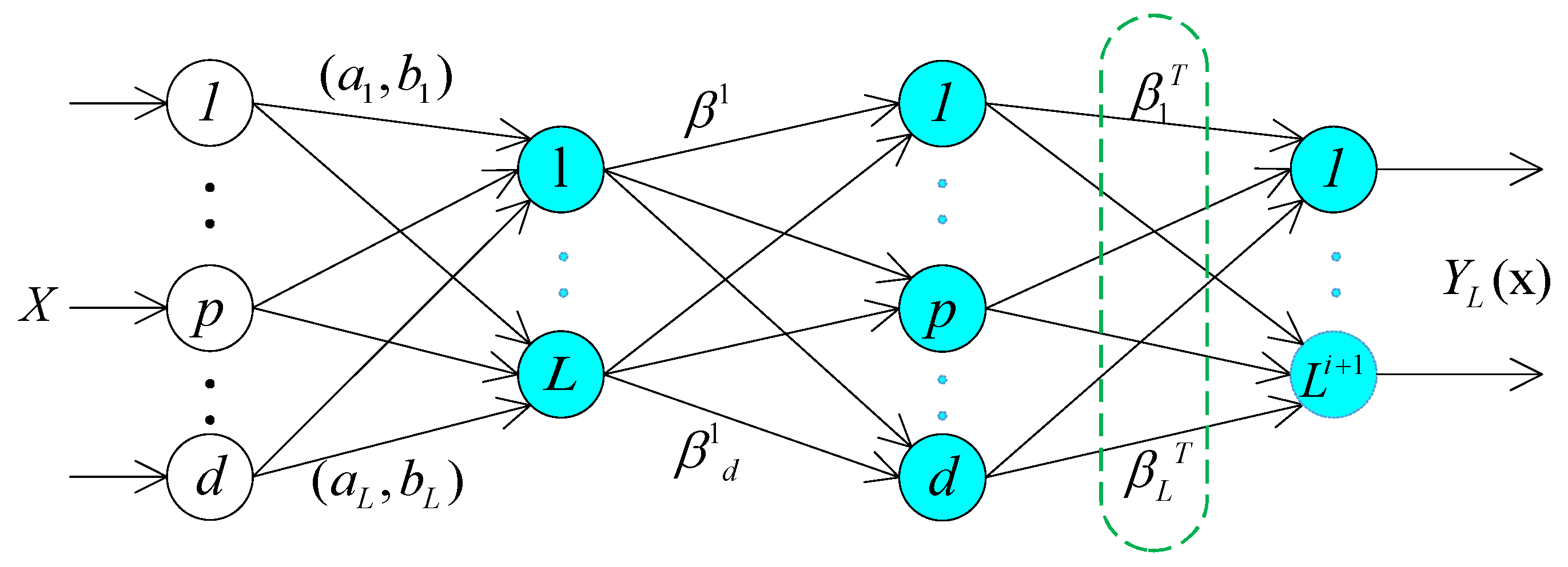
2.1. Extreme Learning Machines Based Autoencoder
- (1)
- Compressed representation: represent features from a high dimensional input data space to a low dimensional feature space;
- (2)
- Sparse representation: represent features from a low dimensional input data space to a high dimensional feature space;
- (3)
- Equal representation: represent features from an input data space dimension equal to feature space dimension.
2.2. Dimension Compression
- (1)
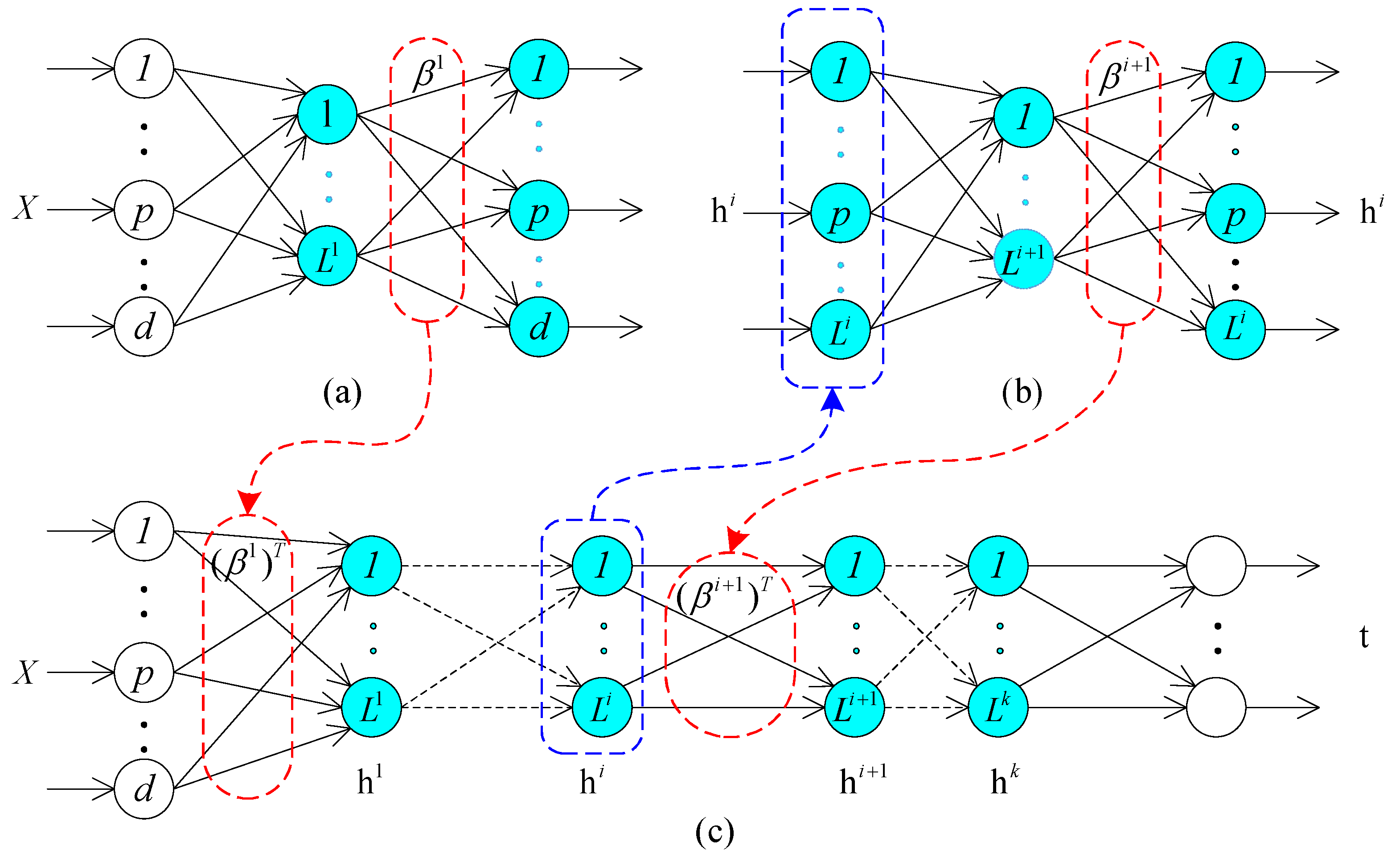
- The proposed autoencoder is a ELM based network composing of a set of single-hidden-layer slice, whereas the DL-based autoencoder is a multiple hidden layers network.
- (2)
- DL tends to adopt BP algorithm to train all parameters of autoencoder, differently, this paper employs the ELM to configure the network with supervised learning (i.e., Let the output data equal to input data, ). We can get the final output weight so as to transform input data into a new representation through Equation (8). The dimension of converted data is much smaller than the raw input data.
- (3)
- The DL-based autoencoder tends to map the input dataset into high-dimensional sparse features. While this research applies a compressed representation of the input data.
- (4)
- The DL-based autoencoder trained with BP algorithm is a really time-consuming process as it requires intensive parameters setting and iterative tuning. On the contrary, each ELM slice in the multi-layered ELM based autocoder can be seen as an independent feature extractor, which relies only on the feature output of its previous hidden layer. The weights or parameters of the current hidden layer could be assigned randomly.
2.3. ELM for Classification
- (1)
- If the ELM only has a single-output node, among the multiclass labels, ELM selects the most closed value as the target label. In this case, the ELM solution to the binary classification case becomes a specific case of multiclass solution.
- (2)
- If the ELM has multi-output nodes, the index of the output node with the highest output value is considered as the label of the input data.
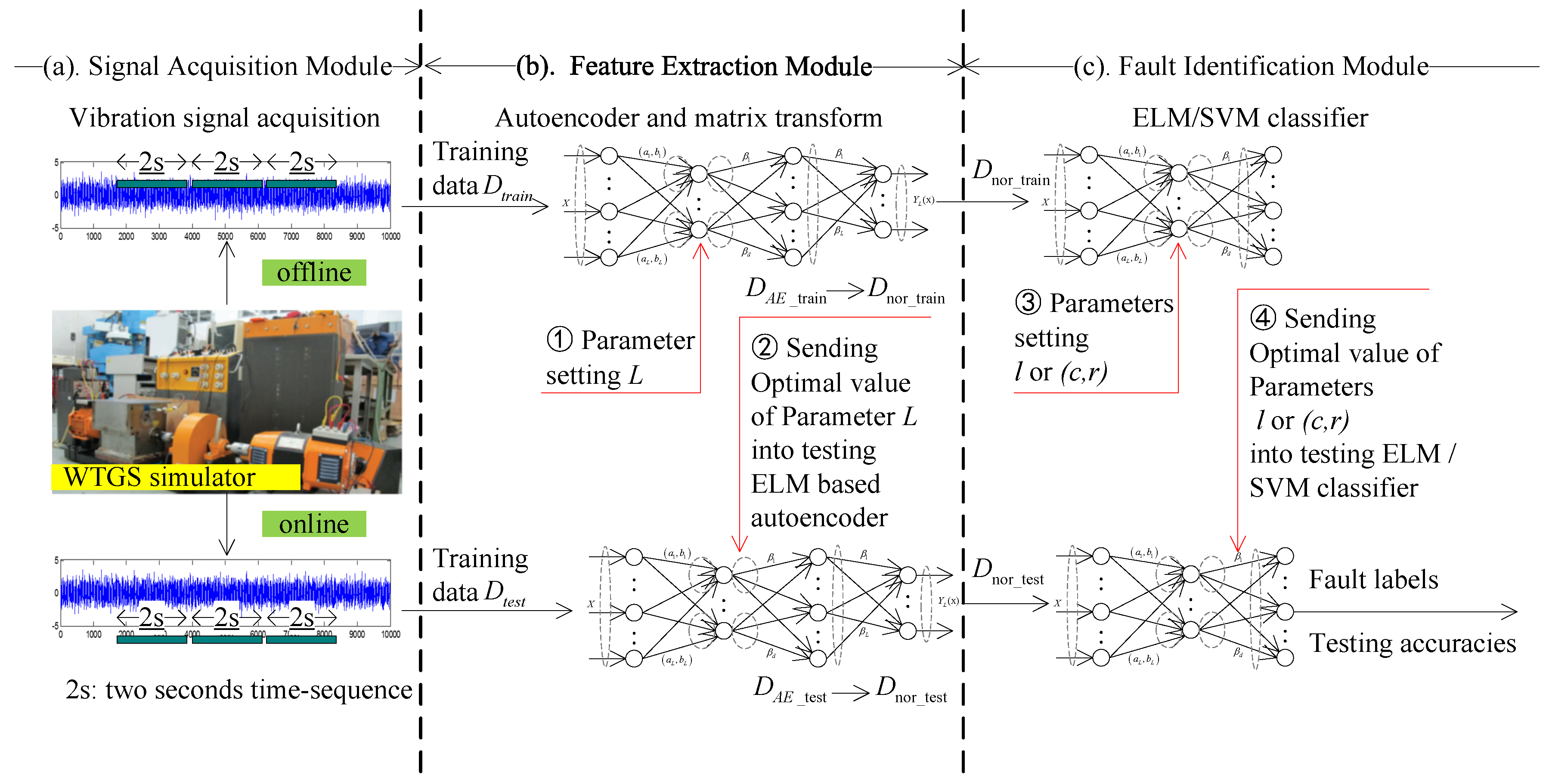
2.4. General Workflow
3. Case Study and Experimental Setup
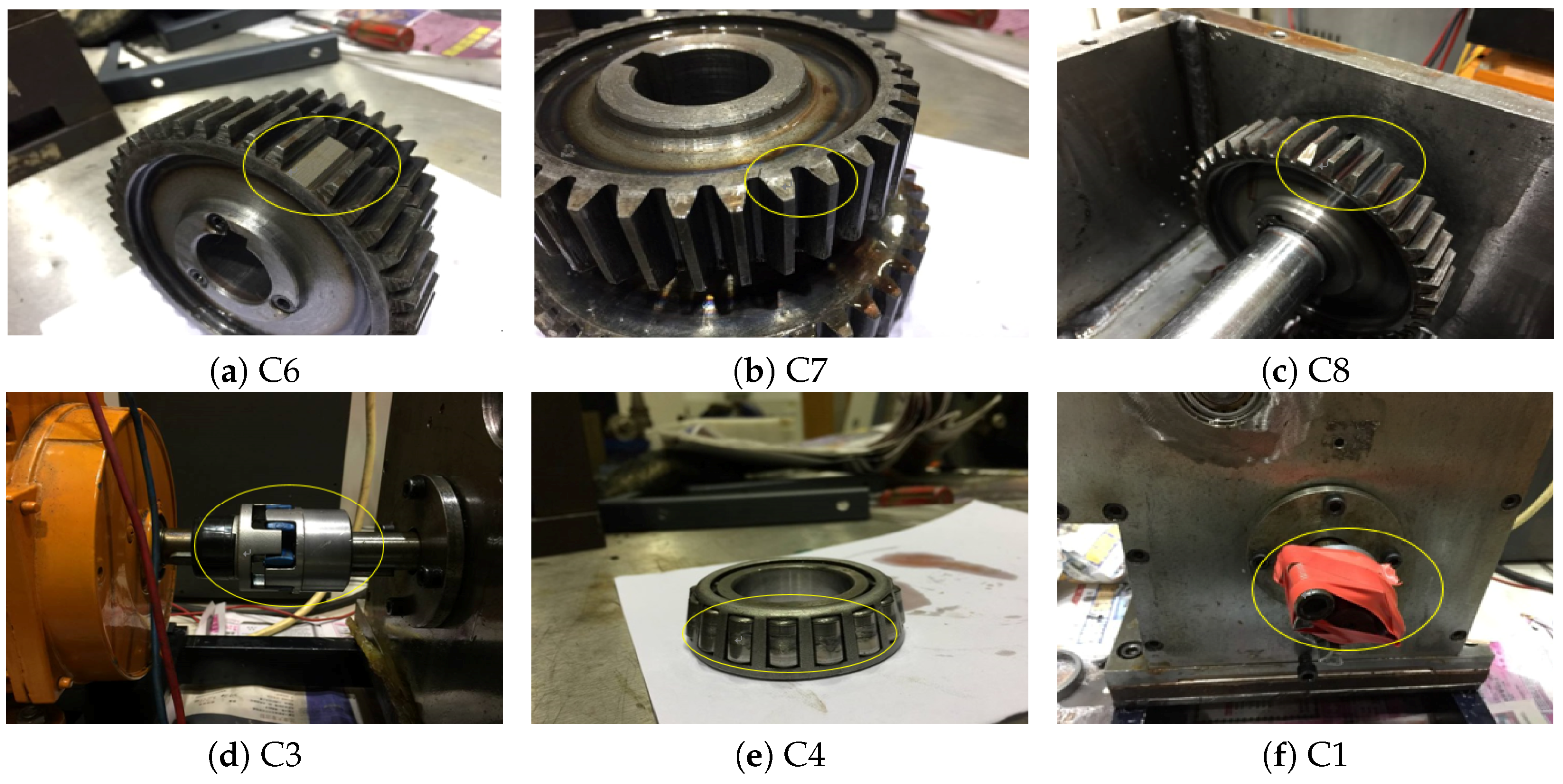
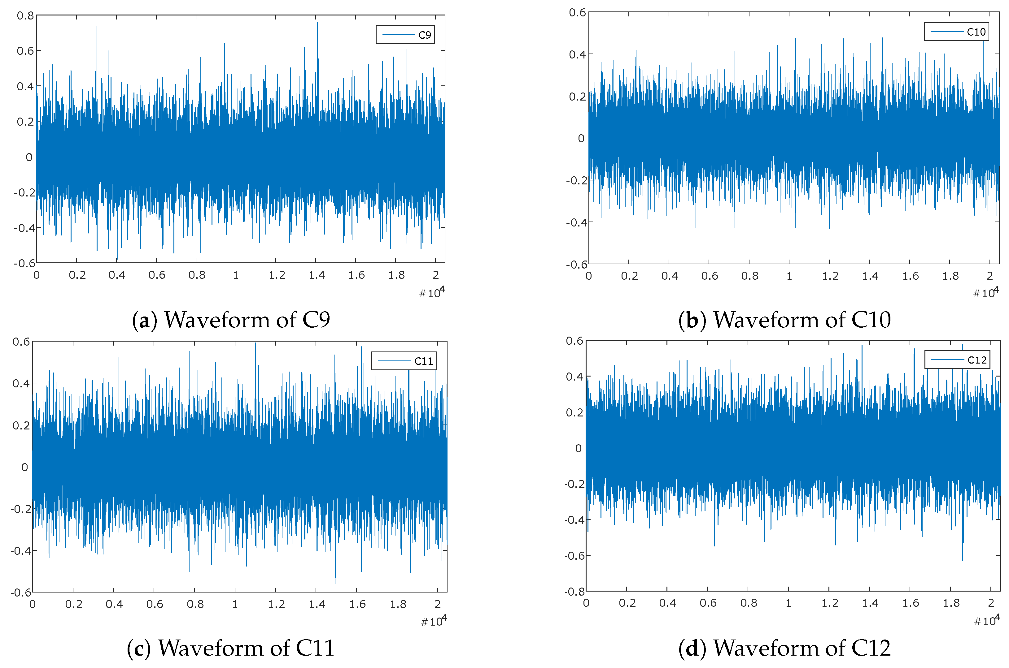
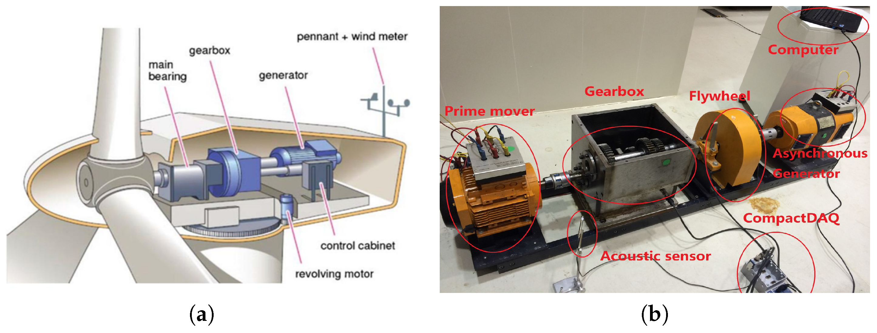
3.1. Test Rig and Signals Acquisition
3.2. Feature Extraction and Dimension Reduction
4. Experimental Results and Discussion
5. Conclusions
Acknowledgments
Author Contributions
Conflicts of Interest
References
- Amirat, Y.; Benbouzid, M.E.H.; Al-Ahmar, E.; Bensaker, B.; Turri, S. A brief status on condition monitoring and fault diagnosis in wind energy conversion systems. Renew. Sustain. Energy Rev. 2009, 13, 2629–2636. [Google Scholar] [CrossRef]
- Yin, S.; Luo, H.; Ding, S.X. Real-time implementation of fault-tolerant control systems with performance optimization. IEEE Trans. Ind. Electron. 2014, 61, 2402–2411. [Google Scholar] [CrossRef]
- Wong, P.K.; Yang, Z.; Vong, C.M.; Zhong, J. Real-time fault diagnosis for gas turbine generator systems using extreme learning machine. Neurocomputing 2014, 128, 249–257. [Google Scholar] [CrossRef]
- Yan, R.; Gao, R.X.; Chen, X. Wavelets for fault diagnosis of rotary machines: A review with applications. Signal Process. 2014, 96, 1–15. [Google Scholar] [CrossRef]
- Fan, W.; Cai, G.; Zhu, Z.; Shen, C.; Huang, W.; Shang, L. Sparse representation of transients in wavelet basis and its application in gearbox fault feature extraction. Mech. Syst. Signal Process. 2015, 56, 230–245. [Google Scholar] [CrossRef]
- Vincent, P.; Larochelle, H.; Bengio, Y.; Manzagol, P.A. Extracting and composing robust features with denoising autoencoders. In Proceedings of the 25th International Conference on Machine Learning, Helsinki, Finland, 5–9 July 2008; pp. 1096–1103.
- Bianchi, D.; Mayrhofer, E.; Gröschl, M.; Betz, G.; Vernes, A. Wavelet packet transform for detection of single events in acoustic emission signals. Mech. Syst. Signal Process. 2015. [Google Scholar] [CrossRef]
- Keskes, H.; Braham, A.; Lachiri, Z. Broken rotor bar diagnosis in induction machines through stationary wavelet packet transform and multiclass wavelet SVM. Electric Power Syst. Res. 2013, 97, 151–157. [Google Scholar] [CrossRef]
- Li, N.; Zhou, R.; Hu, Q.; Liu, X. Mechanical fault diagnosis based on redundant second generation wavelet packet transform, neighborhood rough set and support vector machine. Mech. Syst. Signal Process. 2012, 28, 608–621. [Google Scholar] [CrossRef]
- Wang, Y.; Xu, G.; Liang, L.; Jiang, K. Detection of weak transient signals based on wavelet packet transform and manifold learning for rolling element bearing fault diagnosis. Mech. Syst. Signal Process. 2015, 54, 259–276. [Google Scholar] [CrossRef]
- Ebrahimi, F.; Setarehdan, S.K.; Ayala-Moyeda, J.; Nazeran, H. Automatic sleep staging using empirical mode decomposition, discrete wavelet transform, time-domain, and nonlinear dynamics features of heart rate variability signals. Comput. Methods Prog. Biomed. 2013, 112, 47–57. [Google Scholar] [CrossRef] [PubMed]
- Khorshidtalab, A.; Salami, M.J.E.; Hamedi, M. Robust classification of motor imagery EEG signals using statistical time–domain features. Physiol. Meas. 2013, 34. [Google Scholar] [CrossRef] [PubMed]
- Li, W.; Zhu, Z.; Jiang, F.; Zhou, G.; Chen, G. Fault diagnosis of rotating machinery with a novel statistical feature extraction and evaluation method. Mech. Syst. Signal Process. 2015, 50, 414–426. [Google Scholar] [CrossRef]
- Allen, E.A.; Erhardt, E.B.; Wei, Y.; Eichele, T.; Calhoun, V.D. Capturing inter-subject variability with group independent component analysis of fMRI data: a simulation study. Neuroimage 2012, 59, 4141–4159. [Google Scholar] [CrossRef] [PubMed]
- Du, K.L.; Swamy, M. Independent component analysis. In Neural Networks and Statistical Learning; Springer: New York, NY, USA, 2014; pp. 419–450. [Google Scholar]
- Shlens, J. A tutorial on principal component analysis. Available online: http://arxiv.org/pdf/1404.1100v1.pdf (accessed on 7 April 2014).
- Waldmann, I.P.; Tinetti, G.; Deroo, P.; Hollis, M.D.; Yurchenko, S.N.; Tennyson, J. Blind extraction of an exoplanetary spectrum through independent component analysis. Astrophys. J. 2013, 766. [Google Scholar] [CrossRef]
- Mairal, J.; Bach, F.; Ponce, J. Task-driven dictionary learning. IEEE Trans. Pattern Anal. Mach. Intell. 2012, 34, 791–804. [Google Scholar] [CrossRef] [PubMed]
- Lei, Y.; He, Z.; Zi, Y.; Chen, X. New clustering algorithm-based fault diagnosis using compensation distance evaluation technique. Mech. Syst. Signal Process. 2008, 22, 419–435. [Google Scholar] [CrossRef]
- Bro, R.; Smilde, A.K. Principal component analysis. Anal. Methods 2014, 6, 2812–2831. [Google Scholar] [CrossRef]
- Xanthopoulos, P.; Pardalos, P.M.; Trafalis, T.B. Principal component analysis. In Robust Data Mining; Springer: New York, NY, USA, 2013; pp. 21–26. [Google Scholar]
- Hoque, M.S.; Mukit, M.; Bikas, M.; Naser, A. An implementation of intrusion detection system using genetic algorithm. Int. J. Netw. Secur. 2012, 4, 109–120. [Google Scholar]
- Johnson, P.; Vandewater, L.; Wilson, W.; Maruff, P.; Savage, G.; Graham, P.; Macaulay, L.S.; Ellis, K.A.; Szoeke, C.; Martins, R.N. Genetic algorithm with logistic regression for prediction of progression to Alzheimer’s disease. BMC Bioinform. 2014, 15. [Google Scholar] [CrossRef] [PubMed]
- Whitley, D. An executable model of a simple genetic algorithm. Found. Genet. Algorithms 2014, 2, 45–62. [Google Scholar]
- Tang, J.; Deng, C.; Huang, G.B. Extreme Learning Machine for Multilayer Perceptron. IEEE Trans. Neural Netw. Learn. Syst. 2015, 27, 809–821. [Google Scholar] [CrossRef] [PubMed]
- Hinton, G.E. A practical guide to training restricted boltzmann machines. In Neural Networks: Tricks of the Trade; Springer: Lake Tahoe, NV, USA, 2012; pp. 599–619. [Google Scholar]
- Srivastava, N.; Salakhutdinov, R.R. Multimodal learning with deep boltzmann machines. In Advances in Neural Information Processing Systems; Springer: Lake Tahoe, NV, USA, 2012; pp. 2222–2230. [Google Scholar]
- Fischer, A.; Igel, C. An introduction to restricted Boltzmann machines. In Progress in Pattern Recognition, Image Analysis, Computer Vision, and Applications; Springer: Buenos Aires, Argentina, 2012; pp. 14–36. [Google Scholar]
- Yang, Z.; Wong, P.K.; Vong, C.M.; Zhong, J.; Liang, J. Simultaneous-fault diagnosis of gas turbine generator systems using a pairwise-coupled probabilistic classifier. Math. Probl. Eng. 2013, 2013. [Google Scholar] [CrossRef]
- Vong, C.M.; Wong, P.K. Engine ignition signal diagnosis with wavelet packet transform and multi-class least squares support vector machines. Expert Syst. Appl. 2011, 38, 8563–8570. [Google Scholar] [CrossRef]
- Abbasion, S.; Rafsanjani, A.; Farshidianfar, A.; Irani, N. Rolling element bearings multi-fault classification based on the wavelet denoising and support vector machine. Mech. Syst. Signal Process. 2007, 21, 2933–2945. [Google Scholar] [CrossRef]
- Widodo, A.; Yang, B.S. Application of nonlinear feature extraction and support vector machines for fault diagnosis of induction motors. Expert Syst. Appl. 2007, 33, 241–250. [Google Scholar] [CrossRef]
- Sankari, Z.; Adeli, H. Probabilistic neural networks for diagnosis of Alzheimer’s disease using conventional and wavelet coherence. J. Neurosci. Methods 2011, 197, 165–170. [Google Scholar] [CrossRef] [PubMed]
- Othman, M.F.; Basri, M.A.M. Probabilistic neural network for brain tumor classification. In Proceedings of the 2011 Second International Conference on Intelligent Systems, Modelling and Simulation (ISMS), Kuala Lumpur, Malaysia, 25–27 January 2011; pp. 136–138.
- Huang, G.B.; Zhou, H.; Ding, X.; Zhang, R. Extreme learning machine for regression and multiclass classification. IEEE Trans. Syst. Man Cybern. Part B Cybern. 2012, 42, 513–529. [Google Scholar] [CrossRef] [PubMed]
- Huang, G.B.; Ding, X.; Zhou, H. Optimization method based extreme learning machine for classification. Neurocomputing 2010, 74, 155–163. [Google Scholar] [CrossRef]
- Huang, G.B.; Zhu, Q.Y.; Siew, C.K. Extreme learning machine: theory and applications. Neurocomputing 2006, 70, 489–501. [Google Scholar] [CrossRef]
- Huang, G.B. What are Extreme Learning Machines? Filling the Gap Between Frank Rosenblatt’s Dream and John von Neumann’s Puzzle. Cognit. Comput. 2015, 7, 263–278. [Google Scholar] [CrossRef]
- Wong, P.K.; Wong, K.I.; Vong, C.M.; Cheung, C.S. Modeling and optimization of biodiesel engine performance using kernel-based extreme learning machine and cuckoo search. Renew. Energy 2015, 74, 640–647. [Google Scholar] [CrossRef]
- Luo, J.; Vong, C.M.; Wong, P.K. Sparse bayesian extreme learning machine for multi-classification. IEEE Trans. Neural Netw. Learn. Syst. 2014, 25, 836–843. [Google Scholar] [PubMed]
- Cambria, E.; Huang, G.B.; Kasun, L.L.C.; Zhou, H.; Vong, C.M.; Lin, J.; Yin, J.; Cai, Z.; Liu, Q.; Li, K.; et al. Extreme learning machines [trends and controversies]. IEEE Intell. Syst. 2013, 28, 30–59. [Google Scholar] [CrossRef]
- Widrow, B.; Greenblatt, A.; Kim, Y.; Park, D. The No-Prop algorithm: A new learning algorithm for multilayer neural networks. Neural Netw. 2013, 37, 182–188. [Google Scholar] [CrossRef] [PubMed]
- Bartlett, P.L. The Sample Complexity of Pattern Classification with Neural Networks: The Size of the Weights is More Important than the Size of the Network. IEEE Trans. Inf. Theory 1998, 44, 525–536. [Google Scholar] [CrossRef]


| The ELM Training Algorithm |
|---|
| Step1, Initializing the hidden nodes L; |
| Step2, Randomly assign input weight and bias ; |
| Step3, Calculate the hidden layer output matrix ; |
| Step4, Calculate the output weight vector ; |
| Step5, Calculate the matrix (as shown in eqs (8) and (9)); |
| Step6, Initializing the hidden nodes l; |
| Step7, Randomly assign input weight and bias ; |
| Step8, Calculate the hidden layer output matrix ; |
| Step9, Calculate the output weight matrix . |
| Case No. | Condition | Fault Description |
|---|---|---|
| C0 | Normal | Normal |
| C1 | Single fault | Unbalance |
| C2 | Looseness | |
| C3 | Mechanical misalignment | |
| C4 | Wear of cage and rolling elements of bearing | |
| C5 | Wear of outer race of bearing | |
| C6 | Gear tooth broken | |
| C7 | Gear crack | |
| C8 | Chipped tooth | |
| C9 | Simultaneous fault | Gear tooth broken and chipped tooth |
| C10 | Chipped tooth and wear of outer race of bearing | |
| C11 | Gear tooth broken and wear of cage and rolling elements of bearing | |
| C12 | Gear tooth broken and wear of cage and rolling elements of bearing and wear of outer race of bearing |
| Dataset | Type of Dataset | Single Fault | Simultaneous Fault |
|---|---|---|---|
| Raw sample data | Training dataset | (1600) | (200) |
| Test dataset | (200) | (80) | |
| Feature extraction (SAE) | Training dataset | (1600) | (200) |
| Test dataset | (200) | (80) |
| Features | Equation | Features | Equation |
|---|---|---|---|
| Mean | Kurtosis | ||
| Standard deviation | Crest factor | ||
| Root mean square | Clearance factor | ||
| Peak | Shape factor | ||
| Skewness | Impulse factor |
| Feature Extraction | Classifier | Accuracies for Test Case (%) | ||
|---|---|---|---|---|
| Single-Fault | Simultaneous-Fault | Overall Fault | ||
| WPT+TDSF+KPCA | PNN | 83.64 | 83.64 | 83.76 |
| RVM | 82.99 | 74.64 | 81.21 | |
| SVM | 92.88 | 89.73 | 90.78 | |
| ELM | 91.29 | 89.72 | 90.89 | |
| EMD+TDSF | PNN | 85.64 | 84.64 | 84.52 |
| RVM | 83.99 | 77.64 | 83.21 | |
| SVM | 95.83 | 92.87 | 94.35 | |
| ELM | 96.20 | 92.44 | 94.32 | |
| LMD+TDSF | PNN | 85.64 | 84.64 | 84.52 |
| RVM | 83.99 | 77.64 | 83.21 | |
| SVM | 95.25 | 92.87 | 93.27 | |
| ELM | 95.83 | 93.04 | 94.44 | |
| ELM-AE | PNN | 85.64 | 84.64 | 84.52 |
| RVM | 83.99 | 77.64 | 83.21 | |
| SVM | 95.83 | 92.87 | 93.27 | |
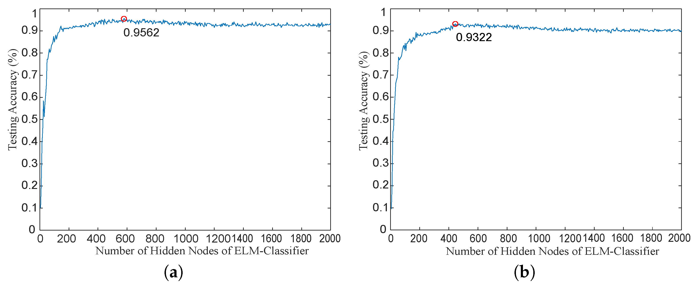
| ELM | 95.62 | 93.22 | 94.42 | |
| Feature Extraction | Fault Type | Accuracies for Test Case (%) | Time for Test Case (ms) | ||
|---|---|---|---|---|---|
| SVM | ELM | SVM | ELM | ||
| ELM-AE | Single-fault | 95.72 ± 2.25 | 95.62 ± 2.25 | 156 ± 0.9 | 18 ± 0.8 |
| Simultaneous-fault | 92.98 ± 1.25 | 93.22 ± 3.25 | 158 ± 0.8 | 20 ± 0.5 | |
| Overall fault | 93.55 ± 3.15 | 94.42 ± 2.75 | 157 ± 0.4 | 20 ± 0.75 | |
© 2016 by the authors; licensee MDPI, Basel, Switzerland. This article is an open access article distributed under the terms and conditions of the Creative Commons Attribution (CC-BY) license (http://creativecommons.org/licenses/by/4.0/).
Share and Cite
Yang, Z.-X.; Wang, X.-B.; Zhong, J.-H. Representational Learning for Fault Diagnosis of Wind Turbine Equipment: A Multi-Layered Extreme Learning Machines Approach. Energies 2016, 9, 379. https://doi.org/10.3390/en9060379
Yang Z-X, Wang X-B, Zhong J-H. Representational Learning for Fault Diagnosis of Wind Turbine Equipment: A Multi-Layered Extreme Learning Machines Approach. Energies. 2016; 9(6):379. https://doi.org/10.3390/en9060379
Chicago/Turabian StyleYang, Zhi-Xin, Xian-Bo Wang, and Jian-Hua Zhong. 2016. "Representational Learning for Fault Diagnosis of Wind Turbine Equipment: A Multi-Layered Extreme Learning Machines Approach" Energies 9, no. 6: 379. https://doi.org/10.3390/en9060379
APA StyleYang, Z.-X., Wang, X.-B., & Zhong, J.-H. (2016). Representational Learning for Fault Diagnosis of Wind Turbine Equipment: A Multi-Layered Extreme Learning Machines Approach. Energies, 9(6), 379. https://doi.org/10.3390/en9060379