How Much Detail Should We Use to Compute Societal Aggregated Exergy Efficiencies?

Abstract

The current method used for calculating societal aggregated exergy efficiencies is reviewed. Cooling is introduced as an end-use category; conversion efficiencies for heating processes are obtained for each energy carrier; and electricity shares per end-use are retrieved for each sector, improving the accuracy of the estimated values of aggregated exergy efficiencies. We show that: (1) cooling uses are a relevant end-use in Portugal and that their introduction decreased overall efficiency by 3.4% in 2009; and (2) disaggregating the heating second law efficiencies for each energy carrier has a significant effect on the aggregated efficiencies of the country, decreasing aggregated efficiency by 1.3% in 2009. We studied two other factors that showed no significant impact on aggregated exergy efficiency: a technological lag of 10 years in the efficiency of stationary mechanical drive devices and the use of a year-specific ambient temperature to compute exergy efficiencies of heating processes.

1. Introduction

Energy consumption worldwide has been increasing at a very high rate, and despite current investments in renewable sources of energy, fossil fuel consumption still plays an important role in the economies of both developed and developing countries. Societal exergy analyses can help the move towards more efficient energy usage by making better use of the natural resources available because they provide a common basis on which to compare different energy vectors and different uses, in terms of their efficiency [1]. Exergy analyses tell us the distance from the ideal process, which relates to (1) a mismatch between the energy carrier (its potential to do work) and the end-use (the work needed to achieve it) and (2) irreversibilities in the process itself.

Societal exergy studies are undertaken at the various stages along the energy flow, namely primary, final and useful energy. The primary to final conversion is mainly related to energy transformations, comprising the energy sector. The final to useful conversion is related to the way energy is used to provide an end-use, such as heat, movement or light. Studies at the level of useful energy are important to understand how well energy is being utilized.

Useful exergy, or useful work analyses, have already been done by a variety of authors at the national level [2,3,4,5,6,7,8,9]. In these studies, diverse approaches are chosen for presenting the results, the choice of parameters and time spans. The method applied in our study follows the approach by [6], which was later used in [7,8] to account for the energy flows from the typical energy carriers: oil, coal, natural gas, combustible renewables and electricity.

The objective of this study is to analyze whether the method currently used to account for useful exergy and final to useful exergy efficiencies at the national level [7,8] should be more detailed. Our focus will be on the: (1) introduction of cooling as a new end-use category; (2) use of heat efficiencies that depend on the energy carrier; and (3) more detailed disaggregation of electricity end-uses per sector.

A sensitivity analysis was performed to evaluate the impact of these changes on aggregated exergy efficiencies. The necessity of being more detailed, regarding the ambient temperature and the efficiency of the stationary mechanical drive, was also assessed. A program was developed in R to use energy data from the International Energy Agency (IEA) energy statistics to compute aggregated final to useful exergy efficiencies. The work was conducted using Portugal as a case study, comprising the period from 1960 to 2009.

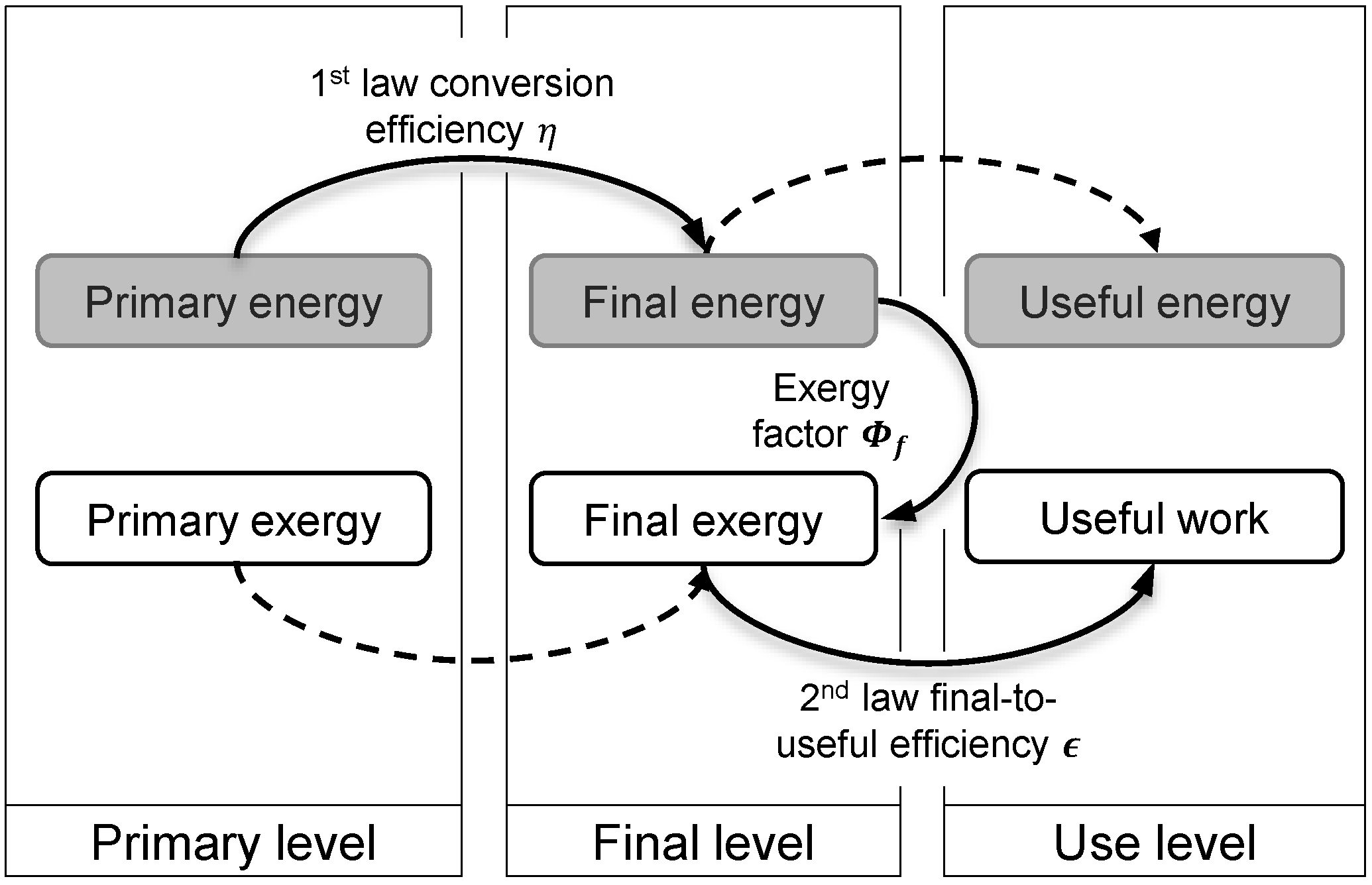
2. Methodology and Data

Final energy data for all energy carriers, with the exception of combustible renewables, was retrieved from the energy statistics from the IEA, while data for combustible renewables was retrieved from [10], due to inconsistencies in this energy vector in the IEA statistics, for Portugal. The IEA database is disaggregated into sectors and sub-sectors of the economy and presents the energy consumption of each energy vector for each of these sub-sectors of the economy. The assumptions that were used to allocate end-uses for each of these pairs of sub-sector/energy vector and to estimate efficiencies are described in the next subsections. Electricity end-uses, for example, are difficult to estimate because electricity can easily be transformed into any other form of energy, and therefore, estimations and approximations for these quantities are required. The method followed to obtain useful exergy from final exergy and aggregated efficiencies for the Portuguese economy is also described in the following subsections. In Figure 1, the conversions between the primary and final stages of energy and exergy are shown. In this paper, the focus is on the conversion from final to useful exergy.

2.1. Final Energy to Final Exergy Data

Energy from statistical data can be converted to exergy data using an exergy factor, which varies with the energy carrier. In

Table 1. Considered exergy factors (values for the exergy factors were taken from [12,13]).

Energy Carriers	Exergy Factors
Coal and coal products	1.06
Oil products	1.06
Coke	1.05
Natural gas	1.04
Combustible renewables	1.11
Electricity	1.00
CHP	0.60

, the exergy factors used in the conversion are presented for the different energy carriers that are included in the IEA energy balances.

In [11], the authors show that the exergy of fuels is similar to the heating-value (HV), where HV is between the lower heating value (LHV) and the higher heating value (HHV). This is consistent with the coefficients given in Table 1, because the IEA energy data used reports the LHV for all fuels with the exception of gases, for which HHV is reported. Natural gas in Portugal has been used from 1997 onwards and represents a small percentage of final energy (a big fraction is used for electricity production); therefore, any correction (the IEA suggests that for gases, the conversion to LHV should be done by multiplying the values that are given by 0.9) would have a negligible impact on the results. The value of the exergy factor given in Table 1 for combined heat and power (CHP) was obtained from the study of [12] assuming that CHP use in Portugal is similar to that of Italy. The service temperature for the exergy factor 0.6 is 600 ${}^{\circ }$C and corresponds to high temperature CHP.

Exergy factors take into account the fact that exergy distinguishes work from heat, giving energy a grade of quality [7]. Electricity can, in theory, be fully converted to work, which is why an exergy factor of one is given to this energy carrier. For fuels, the exergy factor is higher than one because it considers not only the standard enthalpy of combustion, but also the chemical exergy present in the fuel, due to the contribution of post-combustion water vapor within the flue gas components [14].

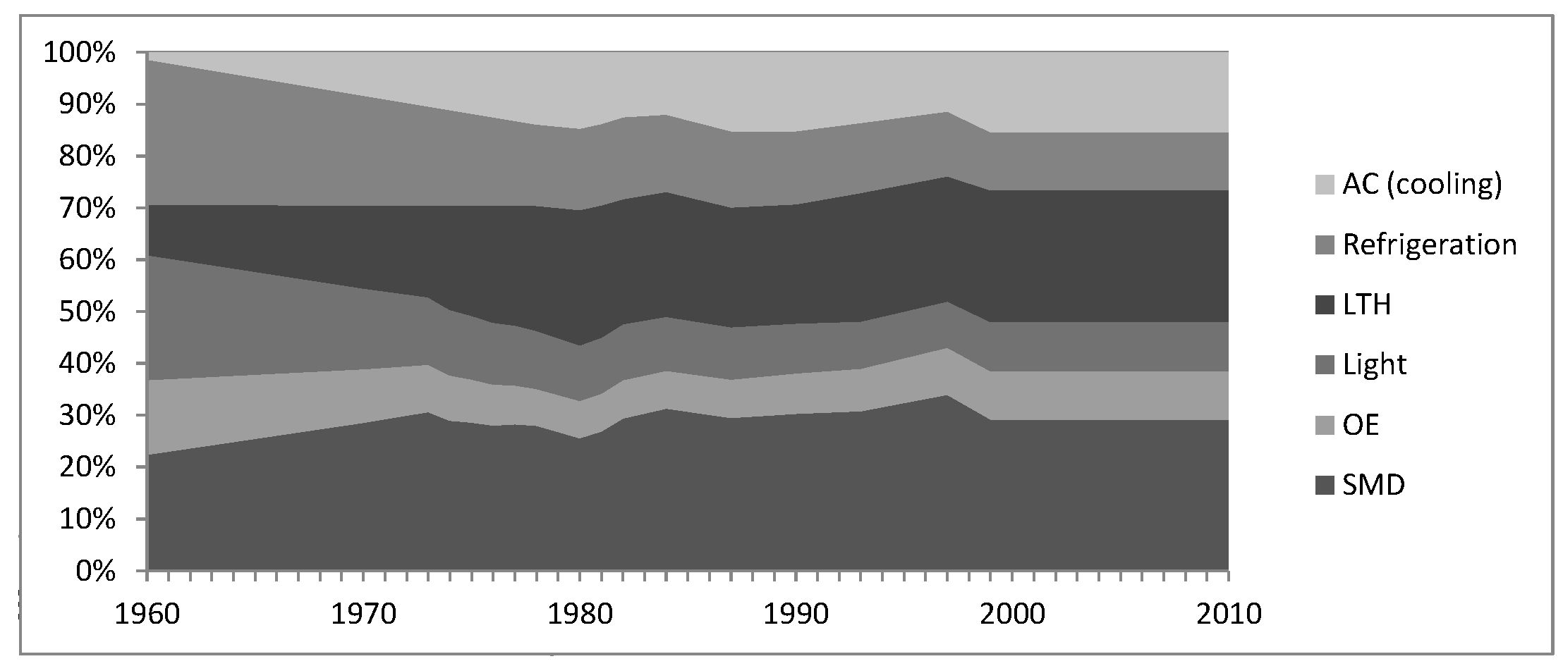
2.2. Allocation of Final Exergy Data to End-Use Categories

The data from IEA have a high level of disaggregation; they are organized for each economic sector by energy carrier, which simplifies the allocation of final energy to end-use categories. The usual end-use categories are heat, mechanical drive (transport and stationary mechanical drive), light and other electric uses. An end-use category that is normally not taken into account is introduced in this paper: cooling.

Cooling has already been used by [9], not as a separate end-use category, but as “stationary mechanical drive”. It is employed in the residential and services sectors during summer for space cooling and throughout the year for the refrigeration of food. In the industrial sector, it is used in the food industry for preservation and likewise in the chemical industries for the preservation of chemical compounds. It also finds uses in the transport sector with air conditioning. Cooling thus has a significant share in the final exergy figures of the economy.

The complete classification of end-use categories, presented in

Table 2. End-use categories for useful exergy calculation.

Aggregated	Disaggregated
Heat	High Temperature Heat	(500 ${}^{°}$ C)
	Medium Temperature Heat	(150 ${}^{°}$ C)
	Low Temperature Heat	(80 ${}^{°}$ C)
Stationary	Oil, mechanical drive
Mechanical	Coal, mechanical drive
Drive	Electricity, mechanical drive
Transport	Steam locomotives
	Diesel vehicles
	Gasoline/LPG vehicles
	Aviation
	Navigation
	Natural gas vehicles
	Diesel-electric
Light
Other electric uses
Cooling	Space cooling
	Refrigeration

, is made according to [6,13], although in these studies, transport and stationary mechanical drives are aggregated into one category (mechanical drive). A proportion of the energy carries, especially in the oil products, is used for non-energy purposes (asphalt, plastics, etc.), which are not accounted for in this study, since they do not provide an energy service. The complete allocation of the economic sectors and sub-sectors of the IEA energy balances to each end-use can be found in the Supplementary Materials.

While the allocation of the final energy carriers, coal, combustible renewables, natural gas, oil products and heat (from cogeneration), for end-uses is done directly according to the industry type, transport type and use in residential, service and miscellaneous sectors, in the case of the allocation of electricity, the information is not readily available, and it changes with time (which does not happen with the allocation of fuels). Electricity (as well as light and cooling uses, which arise from electricity) was treated separately from the other energy carriers, and the shares of utilization per end-use were obtained for each sector and each year from [15]. Such data, despite being collected for the United States of America (USA), are considered an appropriate comparison because of the similarities in developed work electricity usage during the period evaluated (1960 to 2009). In addition, it is a commonly-adopted procedure in similar studies [6,7].

2.3. Estimation of Second Law Efficiencies

To convert the final exergy values obtained in the previous steps to useful exergy values, second law efficiencies are required. The major part of the second law efficiencies depend on the first law efficiencies and on the end-use device type. In [7,8], the useful exergy values were calculated using second law efficiencies that depended mainly on the end-use category and not on the energy carrier. In our study, efficiencies are computed for the energy carrier (end-use pairs), in order to obtain more accurate results. A brief explanation of the second law efficiencies used is given for each end-use category.

2.3.1. Heat

To estimate second law heating efficiencies, service and environment temperatures and first law efficiencies are needed, η:

$$ϵ=\eta ·\left(1-{\displaystyle \frac{T_0}{T_s}}\right)$$

(1)

In this paper, first law efficiencies are estimated by energy carrier, instead of using generalized first law efficiencies for all of the heat processes from all of the energy carriers. The carrier-specific first law efficiencies used by [16] for the European Organization for Economic Co-operation and Development (OECD) countries are used, divided between low, medium and high temperature heat. The energy carriers available for the disaggregation are coal, renewable fuels, oil, natural gas and heat. The evolution of first law efficiencies was assumed equal to the evolution of heat efficiencies used by [7,8].

The service temperatures defined for the heat processes are shown in Table 2. To estimate the second law efficiency for space heating uses, we considered the average winter temperature used by [7] for Portugal. The annual average temperature is 15.4 ${}^{\circ }$C , and the that of the winter is 9.8 ${}^{\circ }$C.

The second law efficiency of low temperature heat uses was multiplied by the exergy allocated to this end-use to obtain useful exergy. The allocation for this end-use in the residential, service and miscellaneous sectors (domestic water and space heating) follows from the assumptions that were mentioned in Section 2.2. Some of the energy carriers used in these sectors, such as “peat briquettes”, are fully allocated to this end-use (for further details, see the Supplementary Materials), while in the case of electricity, only a fraction (dependent on time) is used for this purpose.

2.3.2. Transport

For gasoline engines, the theoretical maximum efficiency depends on the compression ratio, r, and the specific heat ratio, γ, as shown in Equation (2).

$${\eta }_{theoreticalmaximum}=1-{\left(\frac{1}{r}\right)}^{\gamma -1}$$

(2)

The evolution of the compression ratio of gasoline engines during the time span, obtained from [7,17], is used to estimate the theoretical maximum efficiency of these engines. The real (first and second law) efficiency is given by Equation (3), in which the coefficients ${\alpha }_i$ denote losses, which are described in

Table 3. ${\alpha }_i$ loss coefficients for gasoline engines [17,18,19].

Coefficient	Meaning	Approximate Value
1	Reduction due to stoichiometric deviations	0.75
2	Combustion and cylinder wall’s losses	0.75
3	Friction losses	0.85 to 0.90
4	Partial load	0.40 to 0.45
5	Transmission Losses	0.75 (automatic)
		0.90 (manual)

(based on [17,18,19]).

$$ϵ={\eta }_{theoreticalmaximum}·\prod _{i=1}^6{\alpha }_i$$

(3)

In previous studies ([8,20]), a loss coefficient of $0.90$ due to accessories (such as air conditioners (AC)) was included. Here, a different approach is followed, where AC is accounted for directly within LTH or cooling.

Gasoline engine efficiency was used as a starting point to estimate the efficiencies of the other energy carriers used for transport and types of transportation, shown in

Table 4. Efficiencies for transport, per energy carrier.

Energy Carrier	Source
Diesel	$25\%$ more efficient than gasoline [18,21]
Fuel oil	same as gasoline, no ${\alpha }_4$ and ${\alpha }_5$ losses
Ethanol	$20\%$ less efficient than gasoline
Aviation gasoline	[21]
Kerosene	[21]
Steam locomotives	[22,23]
Natural gas	[24]

. As mentioned in [21] and for the same compression ratios, the efficiency attained in ideal Otto cycles is effectively greater than the efficiency obtained in ideal diesel cycles. However, diesel cycles have greater compression ratios, therefore achieving higher efficiencies. The estimated difference is a 25 percent higher efficiency for diesel engines [18]. The values of the efficiencies can be found in the Supplementary Materials.

2.3.3. Stationary Mechanical Drive

The efficiencies of internal combustion engines, used in stationary mechanical drives (SMD), are assumed to be equal to the efficiencies of navigation engines based on the assumption that stationary engines work in a constant regime, as opposed to car engines, which mainly operate in acceleration/deceleration modes. Therefore, there are no losses for partial load (${\alpha }_4$ = 1), and accessories and transmissions losses are also not considered (${\alpha }_5$ = 1, ${\alpha }_6$ = 1). Constant regimes lead to a more efficient use of navigation engines, as well as stationary internal combustion engines [18]. The gasoline SMD efficiencies were assumed to be 25 percent lower than diesel’s.

2.3.4. Light

Light efficiencies are defined differently from all of the others, due to the fact that they are not measured in energy units, but in lumens per watt (light emission per energy input). Light emission is seen by humans in the visible spectrum, and the rate of emission is called the light flux, which has units of “lumens”. Efficacy can then be measured in terms of lumen-hours per kilowatt [25]. Data for lighting efficacy for the United Kingdom (U.K.) for the last century [26] are used for Portugal, because lighting technologies did not differ considerably in developed countries. An efficacy can be defined as in Equation (4).

$$\eta =\frac{outputoflight}{inputofenergy}$$

(4)

The maximum value for the luminous efficacy is found to be 400 lm/W [8,22], and this is the reference value that is taken for the second law efficiency, calculated as shown by Equation (5).

$$ϵ=\frac{W_{min}}{W_{max}}=\frac{Output/W_{max}}{Output/W_{min}}=\frac{\eta }{{\eta }_{ideal}}=\frac{\eta }{400\frac{lm}{W}}$$

(5)

2.3.5. Electricity

Electricity efficiency data were taken from [15], in which the efficiency of electrical uses in the USA in the period from 1900 to 2010 was studied. Electricity end-uses are divided into seven different subcategories, according to the utilization given: low and high temperature heat, stationary mechanical drive, transport, light, other electric uses and cooling. The other electric use category includes all uses that are not included in the other categories, such as communication and electronic devices and electrochemical uses in industry. Electricity allocated to transport is mainly used in railways. Efficiency data for this category were completed with the work of [24].

2.3.6. Cooling

In previous papers (namely [8,20]), the end-use category for SMD comprised refrigeration, HVAC and cooling devices. A different approach is followed in this paper, taking into account that the real end-use for cooling devices is the cooling of spaces or goods. The previous approach was based on the fact that the electricity is used to power a mechanical movement, such as the rotor in electric motors, or in the case of refrigeration and air conditioning, the compressor and fans, which come under the category of the mechanical drive. However, for refrigeration and air conditioning, the mechanical movement of the compressor is not the end-use. This is an inconsistency in the method used when addressing refrigerators and air conditioning as a stationary mechanical drive and not space heating/cooling.

In this paper, a new category of end-use is created to fix this issue: cooling. The shares of electricity allocated to cooling devices (comprising refrigeration and air conditioning) were retrieved from [15], with estimates for cooling and heating uses for air conditioners. These data are for the USA, and shares for the residential sector are shown in Figure 2. The electricity shares were extrapolated at constant values from 2001 to 2010, because we did not have data regarding this period, and there was no marked tendency regarding the evolution of these shares between 1980 and 2000. The relative importance of exergy consumption for refrigeration systems has been decreasing, although the absolute values have been increasing. However, the use of air conditioning devices has grown to a 15 percent share of electricity consumption in the residential sector.

Air conditioning from electricity is allocated both to cooling and low temperature heat (space heating during winter), and refrigeration uses from electricity are included in the category `cooling’. Air conditioner uses in cars for heating and cooling are also considered, with heating uses (during the winter season) going to the LTH uses and cooling uses (during the summer season) going to the cooling category.

Conversion second law efficiencies for refrigeration and air conditioning end-uses were studied. Refrigerators and air conditioners are quite similar in the working principle and use the same components. The difference relies on refrigerators being enclosed and insulated volumes [15]. Analyzing the cooling and heating devices from a thermodynamic perspective, the coefficient of performance is the first law efficiency indicator.

In

Table 5. First and second law efficiencies for cooling and heating devices. COP, coefficient of performance.

COP and Second Law Efficiency	Cooling	Heating
COP (real)	${\displaystyle \frac{Q_{in}}{P_{in}}}$	${\displaystyle \frac{Q_{out}}{P_{in}}}$
COP (ideal)	${\displaystyle \frac{T_c}{T_0-T_c}}$	${\displaystyle \frac{T_h}{T_h-T_0}}$
2nd law	$CO{P}_{real}\left({\displaystyle \frac{T_0-T_c}{T_c}}\right)$	$CO{P}_{real}\left({\displaystyle \frac{T_h-T_0}{T_h}}\right)$

, the coefficients of performance (COP) for cooling and heating devices are shown. For cooling, $Q_{in}$ is the heat removed from the space being cooled, and $P_{in}$ is the electricity required to power the chiller or compressor. Extracting heat from an enclosed volume to maintain its temperature at $T_c$, with an environmental temperature of $T_0$, has the ideal COP expressed in Table 5. In heating, the final use desired is to provide heat at a temperature $T_h$ in an environment with a colder temperature $T_0$. It is important to correctly define the environmental temperatures for summer and winter, for space climatization, as done in [27], because second law efficiencies for cooling and heating depend on them. The heating exergy efficiency in Portugal when a heat pump is used will vary from that of Norway, even if the same technology is involved, because of the different value used for the winter reference temperature, emphasizing that the best solution might not be the same for all countries.

Typical values for the COP of electrically-driven air conditioners and refrigerators are in the range of two to four [28]. Second law efficiencies, needed to convert final exergy values into useful exergy values, are shown in Table 5.

Values for the environment temperature and the temperatures of the hot and cold air are presented in

Table 6. Temperature parameters used for space heating and cooling efficiencies for Portugal.

Conditioning Mode	Outdoor Temperature (${}^{°}$C)	Indoor Temperature (${}^{°}$C)
Heating	9.8	20
Cooling	28	25

, for Portugal. Data are divided between heating and cooling uses, with the outdoor temperature being the winter temperature for the heating uses and the summer temperature for cooling uses, taken from [13,29]. The indoor air temperatures were taken from the Portuguese legislation for the comfort temperatures for AC in buildings (Regulamento das Características de Comportamento Térmico dos Edifícios (RCCTE) in Decreto de Lei n80/2006 de 4 de April 2006 [30]).

For refrigerators, efficiency is calculated assuming a 1/3 load from the freezer box at −15 ${}^{\circ }$C and a 2/3 load from the cooler box at 4 ${}^{\circ }$C [2].

After applying the mean efficiencies from final to useful, the total useful exergy is then aggregated into different categories according to useful exergy uses, as shown in Table 2.

3. Results and Discussion

3.1. Differences from the Methods Previously Used

The method used to estimate useful exergy values and second law efficiencies is described in the previous section. The main differences included in this study to improve the method and the accuracy of the results are emphasized.

The main difference to the end-use categories is the inclusion of cooling uses. These uses arise from electricity and are related to space cooling uses in all sectors, through air conditioners, and refrigeration uses mainly in the industrial, residential and services sectors. A different and improved allocation of end-uses for the electricity energy carrier is done, including shares of utilization for each of the sectors (industrial, transport, residential, services and miscellaneous), an improvement from the general allocation done before in which there were only two different allocations: for the industrial sector and for all of the other sectors collectively.

In the conversion efficiencies, the heating process efficiencies were disaggregated per energy carrier, as opposed to previous studies, in which the efficiencies for heat processes were constant among energy carriers. Here, higher efficiencies were used for natural gas compared to coal and combustible renewables.

In transport, AC was accounted as an end-use and included in the low temperature heating or cooling end-use categories instead of being considered as a loss.

3.2. Impact on Aggregated Exergy Efficiency

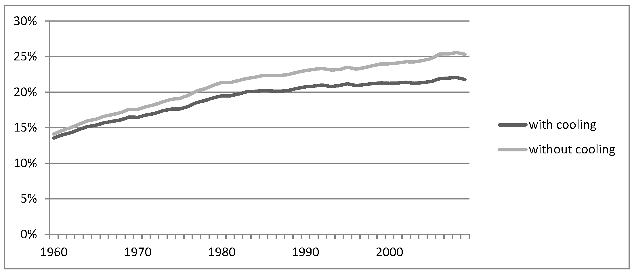
3.2.1. Introduction of the Cooling Category

Cooling is an important end-use category in Portugal. In 2009, it had a seven percent share in final exergy; its share in useful exergy is lower, because of its low conversion efficiency. The percentage of final exergy allocated to cooling has been growing at a constant rate, in line with the increase in the number of cooling devices, including refrigerators and air conditioners, due to their greater incorporation in cars, shopping centers and homes, as people look for solutions to providing thermal comfort.

The effect of the introduction of cooling on the aggregated efficiency of Portugal, shown in Figure 3, was 3.4 percent in 2009 and has been increasing.

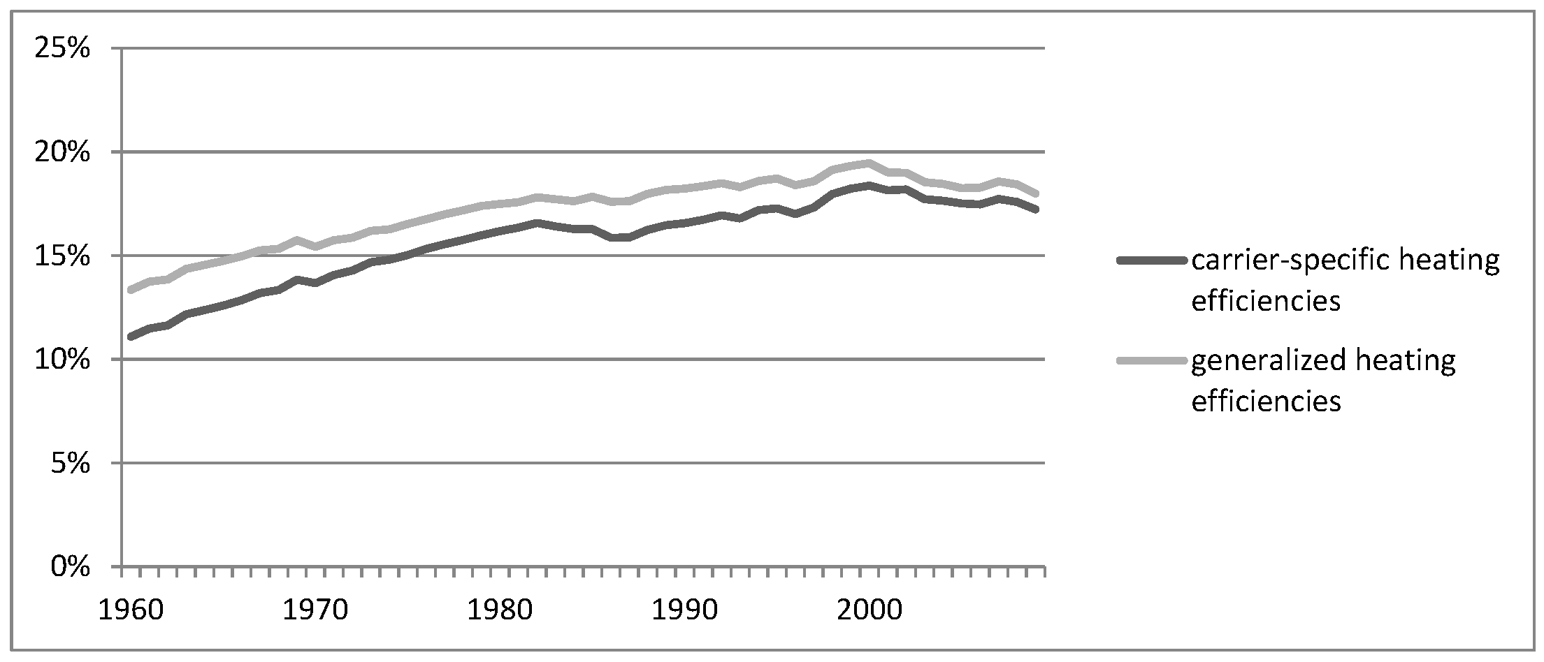
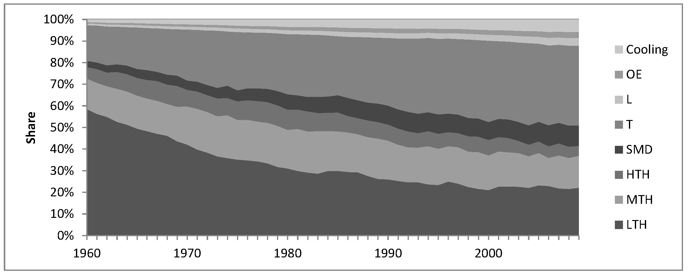
3.2.2. Heating Processes: Carrier Disaggregation

The other main difference from the methodology previously used by [7] is the heating conversion efficiencies. In this paper, a disaggregation of the heating efficiencies by energy carrier is undertaken, to assess if this level of detail is relevant in a useful exergy analysis. The influence of the usage of carrier-specific second law efficiencies is shown in Figure 4.

The difference between the two efficiencies (calculated in an aggregated form for the three heating categories) is more than one percent in some years, being higher in the 1960s and the early 1990s. When using aggregated efficiency, without considering carrier-specific efficiencies for heat processes (red line), some carriers are assigned higher efficiencies than their real values, which is the case for combustible renewables and coal. The useful exergy values calculated for process heat from these carriers (coal and combustible renewables) are higher, bringing the aggregated efficiency up in the 1960s. Since 1997 the effect has been the opposite, since natural gas, which has a higher heating efficiency than oil, is being assigned a lower efficiency, and this has brought the aggregated efficiency down.

3.2.3. Further Disaggregation of Electricity Uses

Electricity uses were subject to a more detailed study, and the shares of end-use per sector were retrieved, providing a more accurate result of the useful exergy distribution per end-use in each of these sectors. The overall impact of using more detailed information on the aggregated second law efficiencies for electricity is shown in Figure 5.

Previously, much electricity was allocated to lighting, which was not realistic. Other electric devices also had a big share in all sectors, and the new information found, from [15], contradicts this. As these two types of uses, lighting and other electric devices, have a very low conversion efficiency, they were bringing efficiency values down, as shown in Figure 5.

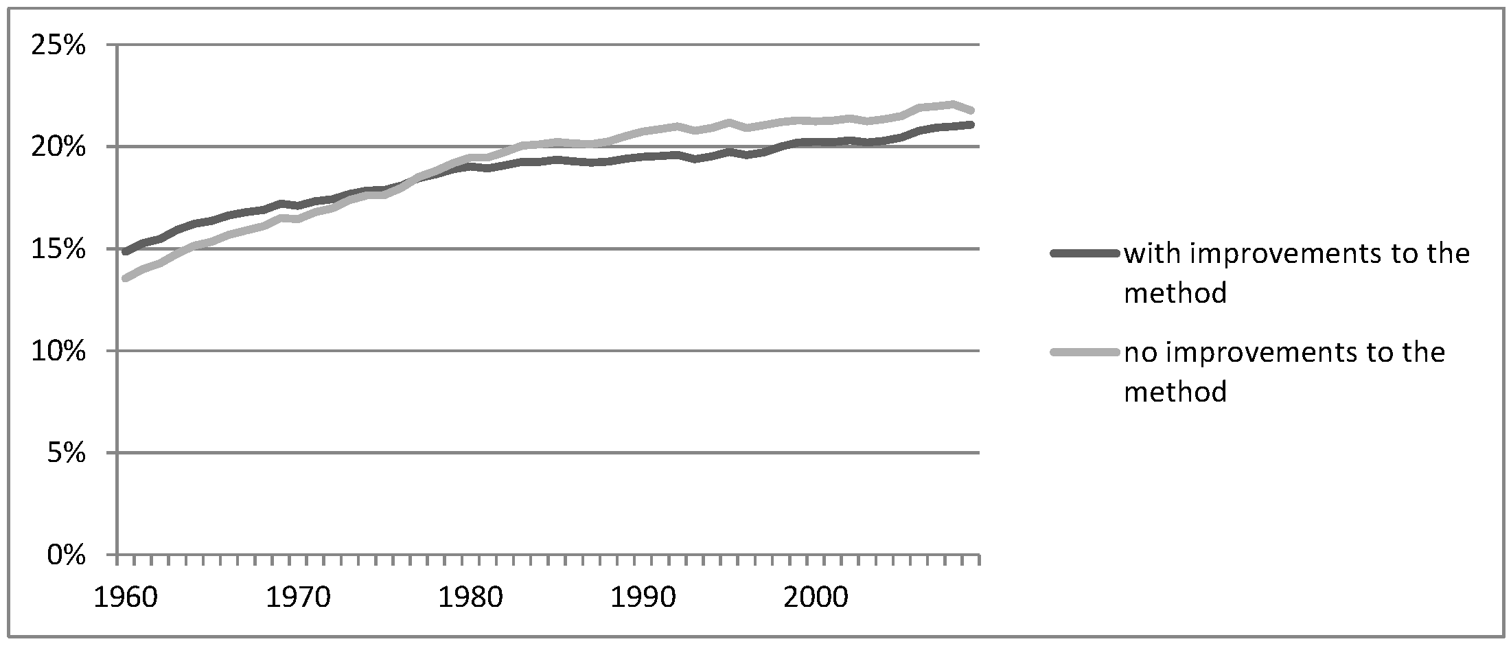
3.2.4. Overall Impact on Aggregated Exergy Efficiency

Figure 6 shows the impact of all improvements on the aggregated second law efficiency.

The allocation of electricity to end-uses undertaken in this study, disaggregated per sector, increased the aggregated efficiency due to the reduction of the allocation to lighting. This has a greater impact during the 1960s, when the effect of the other two modifications was still small. Afterwards, the introduction of cooling and the disaggregation of heating efficiencies per carrier have a greater impact on efficiency reduction, as seen in Figure 3 and Figure 4.

The result of these changes is a more stable evolution of the aggregated second law efficiency, with smoother rather than sudden increases of efficiency (see Figure 6). The evolution of the aggregated second law efficiency is explained by the continuous decrease of the LTH category, which is the least efficient one (see Figure 7), an increase in stationary mechanical drive uses (the most efficient end-use) and a stabilization of the growth of the transport sector (low efficiency).

3.3. Other Factors

3.3.1. SMD

The second law efficiencies used in the calculations of SMD efficiencies were considered as being for USA electric motors, based on the work of [15]. This is the method used in other studies and adopted here. However, not only Portugal is not at the same technological level as the USA, but also engines are not upgraded every year. To evaluate the impact of these inaccuracies, a 10-year delay was applied based on the average life of SMD at homes (dishwashers washing machines, dryers).

The results on the aggregated efficiency are not significant, as seen in Figure 8, with a maximum change in efficiency of 0.2 percent.

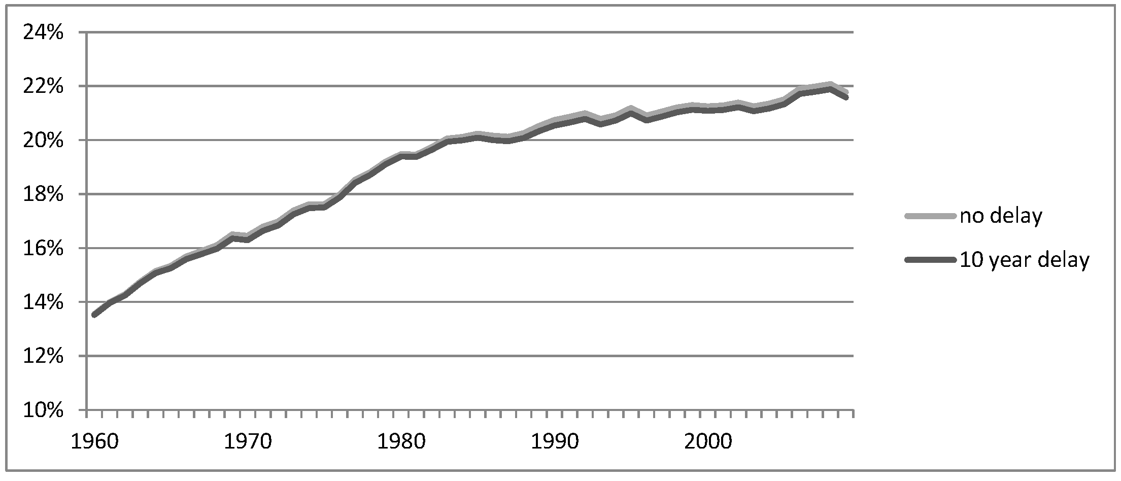
3.3.2. Ambient Temperature Effect on Heating Uses

Heating use exergy efficiencies are highly dependent on the ambient temperature throughout the year. The reference temperature used in this study was constant throughout the data period. The annual and winter averages considered are 15.4 C and 9.8 C (LTH uses), respectively. A sensitivity analysis is performed, using annual-specific temperatures, since 1960. The resulting aggregated efficiency for the whole economy is shown in Figure 9. The change in the aggregated efficiency is not relevant, being at a maximum difference of 0.3 percent in 1963.

4. Conclusions

This paper contributes to an improvement in the method of exergy accounting at the national level, by showing that the inclusion of cooling as an extra useful exergy category and the disaggregation of heating efficiencies per energy carrier have a significant impact on aggregated exergy efficiencies.

Including cooling as an end-use category and analyzing it with specific efficiencies allows for more detailed and accurate aggregated efficiency measures. Portugal’s aggregated efficiency is highly influenced by the introduction of cooling uses, as it is shown by a decrease in 3.4 percent in 2009.

Using the same second law efficiency for heating, for all carriers, inflates the aggregated efficiency for Portugal, in some years, when heating is obtained mainly from coal or combustible renewables, because these carriers tend to have lower conversion efficiencies. On the other hand, in years in which natural gas is more used, which occurred in Portugal since 1997, the aggregated efficiency is deflated because this carrier has higher conversion efficiencies.

Electricity uses were subject to a more detailed allocation using sectoral detailed information. The residential, services and miscellaneous sectors use electricity in different ways; assuming the same use of electricity for all sectors decreases the aggregated efficiency of Portugal.

Additionally, we have shown that the use of (1) improved stationary mechanical drive efficiencies and (2) variable annual ambient temperatures does not have a significant impact on the aggregated efficiency of Portugal.

References

1. Science Europe Physical Chemical and Mathematical Sciences. A Common Scale for Our Common Future: Exergy, a Thermodynamic Metric for Energy; Science Europe Press: Mountain View, CA, USA, 2015. [Google Scholar]
2. Reistad, G. Available Energy Conversion and Utilization in the United States. J. Eng. Gas Turbines Power 1975, 97, 429–434. [Google Scholar] [CrossRef]
3. Wall, G. Exergy conversion in the Swedish society. Resour. Energy 1987, 9, 55–73. [Google Scholar] [CrossRef]
4. Rosen, M. Evaluation of energy utilization efficiency in Canada using energy and exergy analyzes. Energy 1992, 17, 339–350. [Google Scholar] [CrossRef]
5. Ayres, R.; Ayres, L.; Warr, B. Exergy, power and work in the US economy, 1900–1998. Energy 2003, 28, 219–273. [Google Scholar] [CrossRef]
6. Warr, B.; Ayres, R.; Eisenmenger, N.; Krausmann, F.; Schandl, H. Energy use and economic development: A comparative analysis of useful work supply in Austria, Japan, the United Kingdom and the US during 100 years of economic growth. Ecol. Econ. 2010, 69, 1904–1917. [Google Scholar] [CrossRef]
7. Serrenho, A.; Warr, B.; Sousa, T.; Ayres, R.; Domingos, T. Structure and dynamics of useful work along the agriculture-industry-services transition: Portugal from 1856 to 2009. Struct. Chang. Econ. Dyn. 2016, 36, 1–21. [Google Scholar] [CrossRef]
8. Guevara, Z. Three-Level Energy Decoupling: Energy Decoupling at the Primary, Final and Useful Levels of Energy Use. Ph.D. Thesis, Universidade de Lisboa, Lisboa, Portugal, 2014. [Google Scholar]
9. Brockway, P.; Barrett, J.; Foxon, T.; Steinberger, J. Divergence of Trends in US and UK Aggregate Exergy Efficiencies 1960–2010. Environ. Sci. Technol. 2014, 48, 9874–9881. [Google Scholar] [CrossRef] [PubMed]
10. Henriques, S. Energy Transitions, Economic Growth and Structural Change: Portugal in a Long-Run Comparative Perspective; Lund University: Lund, Switzerland, 2011. [Google Scholar]
11. Klein, S.; Nellis, G. Thermodynamics; Cambridge University Press: New York, NY, USA, 2011. [Google Scholar]
12. Wall, G.; Sciubba, E.; Naso, V. Exergy use in the Italian society. Energy 1994, 19, 1267–1274. [Google Scholar] [CrossRef]
13. Serrenho, A.; Sousa, T.; Warr, B.; Ayres, R.; Domingos, T. Decomposition of useful work intensity: The EU (European Union)-15 countries from 1960 to 2009. Energy 2014, 76, 704–715. [Google Scholar] [CrossRef]
14. Cullen, J.; Allwood, J. Theoretical efficiency limits for energy conversion devices. Energy 2010, 35, 2059–2069. [Google Scholar] [CrossRef]
15. Ayres, R.; Ayres, L.; Pokrovsky, V. On the efficiency of US electricity usage since 1900. Energy 2005, 30, 1092–1145. [Google Scholar] [CrossRef]
16. Nakićenović, N.; Gilli, P.; Kurz, R. Regional and global exergy and energy efficiencies. Energy 1996, 21, 223–237. [Google Scholar] [CrossRef]
17. Ford, K.; APS. Efficient Use of Energy: A Physics Perspective; American Institute of Physics: New York, NY, USA, 1975. [Google Scholar]
18. Heywood, J. Internal Combustion Engine Fundamentals; McGraw-Hill: New York, NY, USA, 1988; Volume 930. [Google Scholar]
19. Ross, M. Fuel efficiency and the physics of automobiles. Contemp. Phys. 1997, 38, 381–394. [Google Scholar] [CrossRef]
20. Serrenho, A. Useful Work as an Energy End-Use Accounting Method Historical and Economic Transitions and European Patterns. Ph.D. Thesis, Instituto Superior Técnico, Lisboa, Portugal, 2013. [Google Scholar]
21. Warr, B.; Schandl, H.; Ayres, R. Long term trends in resource exergy consumption and useful work supplies in the UK, 1900 to 2000. Ecol. Econ. 2008, 68, 126–140. [Google Scholar] [CrossRef]
22. Fouquet, R. Heat, Power and Light: Revolutions in Energy Services; Edward Elgar Publishing: Cheltenham, UK, 2008. [Google Scholar]
23. Smil, V. Energy in World History (Essays in World History); Westview Press: Boulder, CO, USA, 1994. [Google Scholar]
24. Ayres, R.; Warr, B. The Economic Growth Engine: How Energy and Work Drive Material Prosperity; Edward Elgar: Cheltenham, UK, 2010. [Google Scholar]
25. Nordhaus, W. Do real-output and real-wage measures capture reality? The history of lighting suggests not. In The Economics of New Goods; University of Chicago Press: Chicago, IL, USA, 1996; pp. 27–70. [Google Scholar]
26. Fouquet, R.; Pearson, P. Seven centuries of energy services: The price and use of light in the United Kingdom (1300–2000). Energy J. 2006, 27, 139–177. [Google Scholar] [CrossRef]
27. Alpuche, M.G.; Heard, C.; Best, R.; Rojas, J. Exergy analysis of air cooling systems in buildings in hot humid climates. Appl. Thermal Eng. 2005, 25, 507–517. [Google Scholar] [CrossRef]
28. Marletta, L. Air conditioning systems from a 2nd law perspective. Entropy 2010, 12, 859–877. [Google Scholar] [CrossRef]
29. Instituto Português do Mar e da Atmosfera. Boletins Climatológicos. 2012. Available online: http://www.ipma.pt/pt/publicacoes/boletins.jsp?cmbDep=clicmbTema=pclidDep=cliidTema=pclcurAno=-1 (accessed on 27 September 2014).
30. Decreto de Lei n80/2006 de 4 de Abril—Diário da República I Série A, Regulamento das Características de Comportamento Térmico dos Edifícios (RCCTE). 2006. Available online: https://dre.pt/application/dir/pdf1sdip/2006/04/067A00/24682513.PDF (accessed on 10 May 2016).
Figure 1. Energy and exergy flows present in a global economic system. Adapted from: [8].
Energies 09 00364 g001
Figure 2. Shares for electricity uses in the residential sector [15].
Energies 09 00364 g002
Figure 3. Effect of the introduction of cooling on the aggregated efficiency.
Energies 09 00364 g003
Figure 4. Aggregated exergy efficiency for the heating categories, considering carrier-specific heat efficiencies.
Energies 09 00364 g004
Figure 5. Electricity exergy efficiency with and without a detailed specification of electricity end-uses per sector.
Energies 09 00364 g005
Figure 6. Aggregated exergy efficiency with the three modifications to the method.
Energies 09 00364 g006
Figure 7. Final exergy per end-use, relative values.
Energies 09 00364 g007
Figure 8. Change in percentage in the aggregated efficiency with a 10-year lag in stationary mechanical drive (SMD) efficiencies applied.
Energies 09 00364 g008
Figure 9. Effect of varying ambient temperatures on Portuguese aggregated efficiency. Ambient temperatures used for the calculation were taken from [29].
Energies 09 00364 g009