Article

Comparison of Moving Boundary and Finite-Volume Heat Exchanger Models in the Modelica Language †

1
Thermodynamics laboratory, University of Liege, Campus du Sart Tilman, B-4000 Liege, Belgium
2
IPU Engineering Consultant, DK-2800 Kongens Lyngby, Denmark
3
Department of Flow heat and combustion Mechanics, University of Gent, 9052 Gent, Belgium
*
Author to whom correspondence should be addressed.
This paper is an extended version of our paper published in Desideri, A.; Wronski, J.; Dechesne, B.; van den Broek, M.; Gusev, S.; Quoilin, S.; Lemort, V. Comparison of moving boundary and finite-volume heat exchanger models in the Modelica language. In the Proceedings of the 3rd International Seminar on ORC Power Systems, Brussels, Belgium, 12–14 October 2015.
Energies 2016, 9(5), 339; https://doi.org/10.3390/en9050339
Submission received: 31 January 2016 / Revised: 11 April 2016 / Accepted: 25 April 2016 / Published: 5 May 2016

Abstract

:
When modeling low capacity energy systems, such as a small size (5–150 kWel) organic Rankine cycle unit, the governing dynamics are mainly concentrated in the heat exchangers. As a consequence, the accuracy and simulation speed of the higher level system model mainly depend on the heat exchanger model formulation. In particular, the modeling of thermo-flow systems characterized by evaporation or condensation requires heat exchanger models capable of handling phase transitions. To this aim, the finite volume (FV) and the moving boundary (MB) approaches are the most widely used. The two models are developed and included in the open-source ThermoCycle Modelica library. In this contribution, a comparison between the two approaches is presented. An integrity and accuracy test is designed to evaluate the performance of the FV and MB models during transient conditions. In order to analyze how the two modeling approaches perform when integrated at a system level, two organic Rankine cycle (ORC) system models are built using the FV and the MB evaporator model, and their responses are compared against experimental data collected on an 11 kWel ORC power unit. Additionally, the effect of the void fraction value in the MB evaporator model and of the number of control volumes (CVs) in the FV one is investigated. The results allow drawing general guidelines for the development of heat exchanger dynamic models involving two-phase flows.

1. Introduction

The crucial role of dynamic modeling tools in tackling the challenges arising from the unsteady operation of complex physical systems has been generally accepted by the scientific community for the simulation of energy systems [1]. Dynamic modeling is considered a reliable tool in energy system design, from evaluating and optimizing the system response time to the development and testing of different control strategies. In recent years, the open-access language Modelica [2] has gained momentum for the dynamic modeling of a wide range of dynamic systems. It allows describing continuous and discrete components in a physical way by writing self-consistent sets of causal and acausal equations that are then transformed by a simulation environment software (e.g., Dymola [3], OpenModelica [4], etc.) into an optimized set of hybrid differential-algebraic equations [5]. Various libraries are available to model thermodynamic and thermal-hydraulic systems [6,7] with a focus on steam and gas cycles (e.g., ThermoSysPro [8], Thermal Power [9], ThermoPower [10], etc.) or refrigeration systems (e.g., TIL Suite [11], Buildings [12], etc.). Some of these libraries are open-access, and only a few of them are able to handle thermo-physical properties of non-conventional working fluids.
The authors recently presented ThermoCycle, a Modelica library targeting the modeling of low-capacity systems [13]. The library aims at providing a robust and efficient fully-open-source suite of models for thermoflow systems, ranging from the computation of thermo-physical substance, through the coupling with the open-source CoolProp software [14], to the simulation of complex systems together with their control strategies.
When modeling low capacity systems, the governing dynamics are usually mainly concentrated in the heat exchanger (HE). In the particular case of heat exchangers involving phase transitions, two commonly-adopted HE modeling approaches are the finite volume (FV) and the moving boundary (MB) [15]. Both methods are based on the conservation laws of energy, mass and momentum over a defined control volume. In a moving boundary model, the fluid flow in the HE is divided into as many control volumes as the states (e.g., liquid, two-phase, vapor) in the fluid flow (in this work: from one to three). The size of the control volumes varies in time during transients, following the saturated liquid and the saturated vapor boundaries. The finite volume approach consists of discretizing the HE volume into a number of equal and constant control volumes. The conservation laws are then applied in each of the control volumes. The MB and FV methods have been applied starting from the late 1970s for thermal system modeling [16,17]. The MB approach results in faster, but sometimes less robust models [15]. Comprehensive literature reviews by [18,19,20], show that moving boundary models have been proposed in several studies, but remain less common than FV models. The work in [21] presents a comparison of the MB and FV modeling approaches for transients in centrifugal chillers. The model results are compared against the experimental data of a 300-kW centrifugal chiller equipped with shell and tube heat exchangers. It is concluded that, while the MB approach results in being three-times faster than the FV one, the assumption of homogeneous flow in the two-phase region over-predicts the void fraction, leading to an under-prediction of the fluid charge. A recent work from [20] reports a clear review of the major MB heat exchanger models capable of handling two-phase flows and presents a moving boundary library developed in the Modelica language for the modeling of direct steam generation parabolic through solar collectors.
This contribution proposes a comparison between the MB and the FV modeling approaches. The models are tested under transient conditions, and their performance is investigated in terms of model integrity by checking the mass and energy balance over a defined simulation time and of model accuracy by comparing the outlet temperature and mass flow rate, considering as a reference a 100-control volumes (CVs) FV model proposed in [22]. The capability of both models to be integrated at a system level is assessed by using both approaches to simulate the evaporator of an organic Rankine cycle (ORC) unit model. The models response is compared against experimental data collected on an 11 kWel ORC test rig. Furthermore, the effect of the void fraction in the MB model and of the number of CVs in the FV model is investigated by means of parametric analyses.
The two types of heat exchanger model are developed in the Modelica language and are included in the open-source ThermoCycle library. The models are developed following an object-oriented approach limiting the use of the Modelica inheritance feature to enhance model readability. Inheritance is a key aspect of the Modelica language, but from the authors’ experience, a massive use of it may lead to puzzling models.
The paper is organized as follows: in Section 2, the modeling approach, the structure and the main characteristic of the FV and MB models are presented. The results of the integrity test are reported in Section 3. In Section 4, the ORC system models are described, and their comparison against transient experimental data is shown together with the performed parametric analysis. The results are finally summarized in Section 5, and some concluding remarks are formulated.

2. Heat Exchanger Modeling

The common assumptions considered for both the finite volume and the moving boundary approaches are reported in Section 2.1. The structure and the governing equations for the MB and the FV models are described in Section 2.2 and Section 2.3, respectively.

2.1. Assumptions

The heat exchanger models presented in this work are conceived of to be integrated into a system model as one of the various components constituting the thermo-hydraulic unit. The following general assumptions for the fluid elements and the metal wall element in the heat exchanger models are considered:
  • The working fluid flow through a control volume of the heat exchanger is described with a mathematical formulation of the conservation laws of physics. Energy and mass balances are expressed considering the dynamic contribution. Given the low time constant characterizing the propagation of pressure throughout the heat exchanger compared to those related to mass and thermal energy transfer, a static momentum balance is assumed.
  • The heat exchanger is considered as a one-dimensional tube (z-direction) in the flow direction.
  • Kinetic energy, gravitational forces and viscous stresses are neglected.
  • No work is done on or generated by the fluid in the control volume.
  • The cross-section area is assumed constant throughout the heat exchanger length.
  • The velocity of the fluid is uniform over the cross-section area (homogeneous two-phase flow).
  • Pressure drops through the heat exchanger are neglected (homogeneous pressure).
  • Axial heat conduction is neglected in the fluid element.
  • The rate of thermal energy addition by radiation is neglected in the fluid element.
  • The rate of thermal energy exchanged with the ambient environment by convection is considered in the fluid element.
  • Thermal energy accumulation is considered for the metal wall of the tube.
  • Thermal energy conduction in the metal wall is neglected in the flow direction and considered static and infinite in the circumferential direction (the wall cross-section area has a uniform temperature).
Other assumptions are taken into account for the secondary fluid side. These assumptions are reported in the next two sections, as they differ depending on the adopted heat exchanger models, i.e., FV or MB.

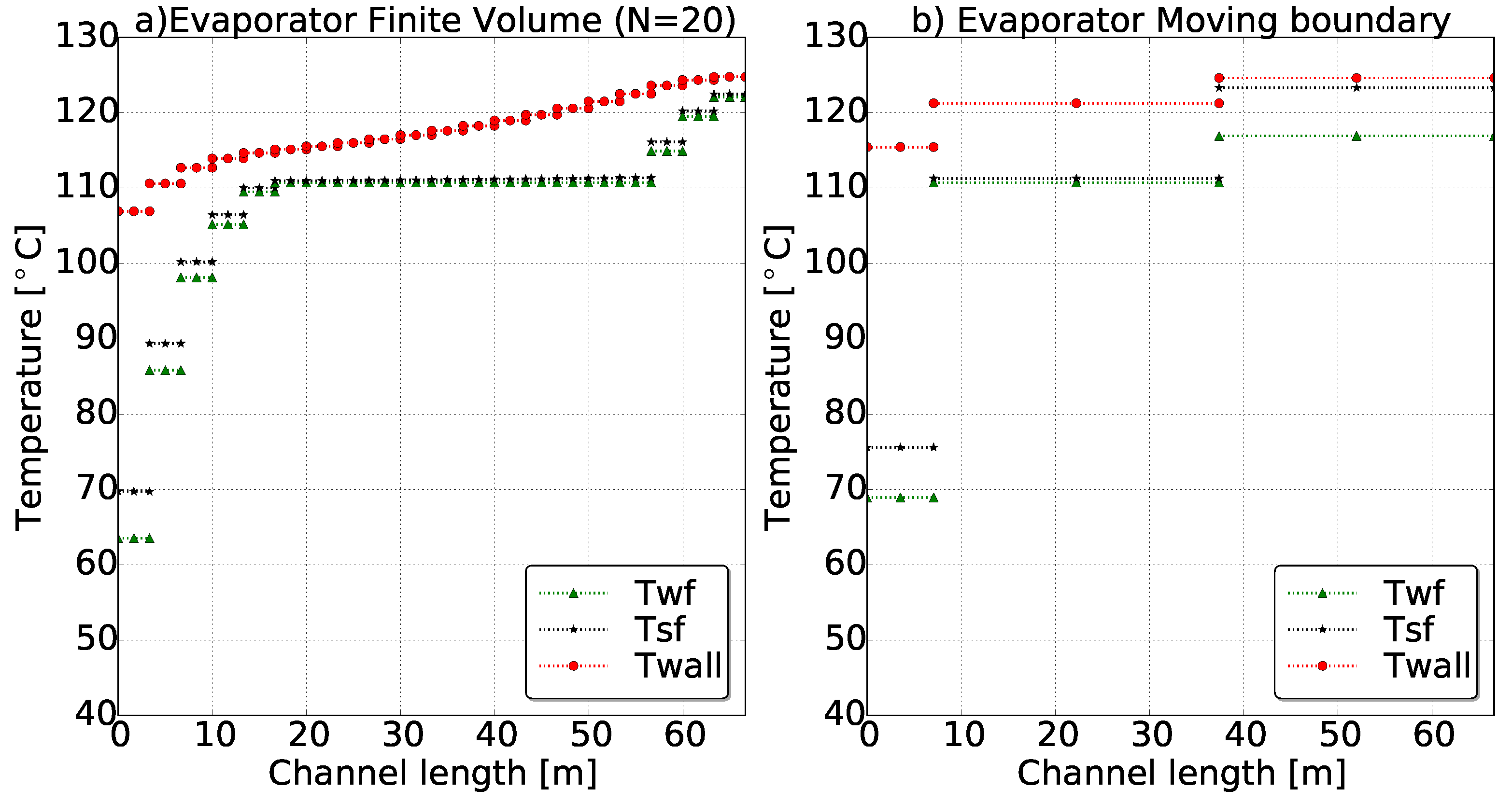
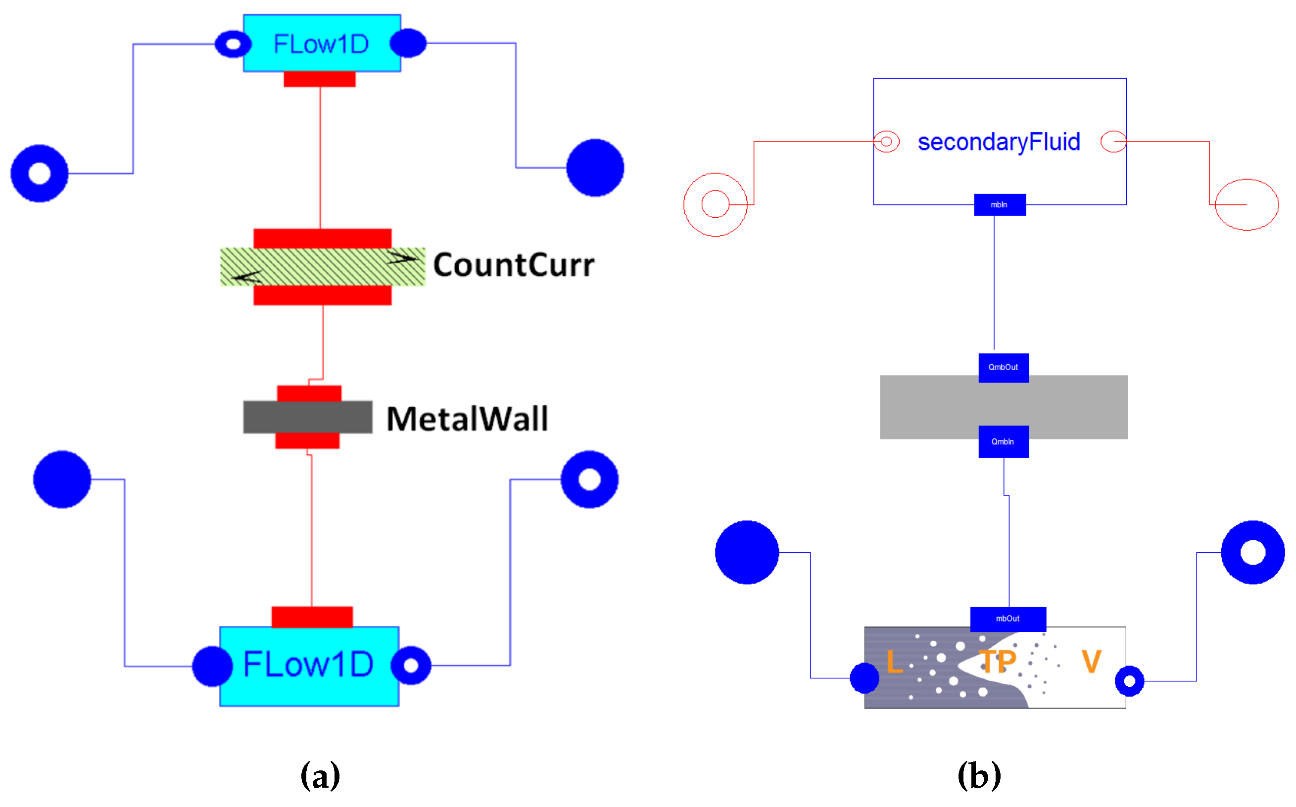
2.2. Finite Volume Model

The finite volume heat exchanger model is object oriented, its structure being shown in Figure 1a. It is based on the connection of different subcomponents from the ThermoCycle library. Two fluid components simulate the flows in the two sides of the heat exchanger, and one wall component accounts for thermal energy accumulation in the metal wall. A forth component CountCurr allows switching between parallel and counter flow configuration. The conservation laws are derived by integrating the general one-dimensional form of mass, energy and momentum balance over a constant volume. Considering the above mentioned assumptions, their final formulation for each CV is reported in Equations (1) to (3), taking p and h as dynamic state variables [23].
d M d t = m ˙ su m ˙ ex with d M d t = V · ρ h · d h d t + ρ p · d p d t
V ρ d h d t = m ˙ su · h su h m ˙ ex · h ex h + V d p d t + A l · q ˙
p su = p ex
where ρ h and ρ p in Equation (1) are considered thermodynamic properties of the fluid and are directly computed by the open-source CoolProp library [14]. The “su” (supply) and “ex” (exhaust) subscripts denote the nodes’ variable of each cell; A l is the lateral surface through which the heat flux q ˙ is exchanged with the metal wall; and V is the constant volume of each cell. Enthalpy and pressure at the center of the control volume are considered as the state variables. The staggered discretization grid is used: the state variables are calculated at the center of the volume, and the node values (“su”,”ex”) are computed based on the selected discretization scheme. Both central and upwind discretization schemes are supported by the model. Thermal energy accumulation in the metal wall is expressed as:
M w N · c w · d T w d t = A ext · q ˙ ext + A int · q ˙ int
where M w is the total mass of the metal wall, N is the number of cells and c w is the metal wall specific heat capacity. The secondary fluid is modeled as an incompressible fluid whose density and specific heat capacity are assumed constant throughout the heat exchanger length. The heat transfer problem between the two fluid components and the metal wall is solved with Newton’s law of cooling. A constant convective heat transfer coefficient is set for the secondary fluid side. In the working fluid side, three constant heat transfer coefficient values are set, one for each region (sub-cooled, two-phase, superheated). The transition between two heat transfer coefficients is based on a non-null quality width by interpolating with a C1 function [23]. The FV model uses the fluid connector from the ThermoCycle library and is compatible with the Modelica Standard library (MSL).

2.3. Moving Boundary Model

The moving boundary model is developed following the object-oriented principles of abstraction, encapsulation and (limited) inheritance: two basic models are formulated simulating the fluid flow through a variable control volume in the single- and two-phase state. The connection of these two basic models allows building dry, flooded or general evaporator and condenser models. The enthalpy distribution of the fluid is assumed linear in each region of the tube (sub-cooled, two-phase, super-heated) and is computed as shown in Equation (5):
h ¯ = 1 2 · h a + h b
where the a and b subscripts denote the left and right boundaries of the region. For a moving boundary control volume, the mass and energy balance are defined by integrating the general conservation laws of physics over the length of the zone, as shown in Equations (6) and (7).
A · l a l b ρ t d z + l a l b m ˙ z d z = 0
A · l a l b ρ · h t d z A · l · d p d t + l a l b h · m ˙ z d z = d l · Y · q ˙
where A is the cross-sectional area, l a and l b are the lengths of the left and right boundaries of the region and Y is the channel perimeter. Assuming a homogeneous pressure, the momentum balance is given by Equation (3). As far as the one-phase region is concerned, the mass balance is derived in Equation (6) by applying the Leibniz rule to the first term and using the mean-value theorem, such that the rate of mass flow change results in:
d d t l a l b ρ d t = d d t ρ ¯ · l
the mass balance for a one-phase region is equal to:
A · ρ ¯ · d l d t + l · d ρ ¯ d t ρ a · d l a d t + ρ b · d l b d t = m ˙ a m ˙ b
where ρ ¯ is the average density of the region computed as a function of the pressure and of the average specific enthalpy, ρ ¯ f h ¯ , p , l is the length of the region and d ρ ¯ d t is calculated as:
d ρ ¯ d t = ρ ¯ p · d p d t + ρ ¯ h ¯ · d h ¯ d t = ρ ¯ p · d p d t + 1 2 · ρ ¯ h ¯ · d h a d t + d h b d t
where d h b / a d t are defined based on Equations (11) to (14) reported in Table 1.
The energy balance is derived from Equation (7). Applying the Leibniz rule to the first term and using the mean-value theorem allows one to define the rate of energy change as:
d d t l a l b ρ · h d z = d d t ρ h ¯ · l d d t ρ ¯ · h ¯ · l
The energy balance for the one-phase region results in:
A · ρ ¯ h ¯ d l d t + h ¯ l d ρ ¯ d t + ρ ¯ l d h ¯ d t + ρ a h a · d l a d t ρ b h b · d l b d t A · l a · d p d t = m ˙ a · h a m ˙ b · h b + Q ˙
In the two-phase region, the assumption of the homogeneous two-phase flow condition allows one to express the mean density as a function of the average void fraction γ ¯ as:
ρ ¯ = 1 γ ¯ ρ l + γ ¯ ρ v
where the average void fraction is calculated integrating the local void fraction γ over the length of the region. γ ¯ is an indicator of the fraction of the total volume of the two-phase region occupied by fluid in the vapor phase [24]. It is derived integrating the void fraction over the two-phase control volume as shown in Appendix A. Substituting Equation (17) into (8) and solving Equation (6) results in the mass balance for the two-phase region:
A ( 1 γ ¯ ) ρ l + γ ¯ ρ v d l d t + l ρ v ρ l d γ ¯ d t + γ ¯ d ρ v d p d p d t + 1 γ ¯ d ρ l d t ρ a d l a d t + ρ b d l b d t = m ˙ a m ˙ b
The energy balance for the two-phase region is obtained from Equation (7) using Equations (17) and (15):
A 1 γ ¯ ρ l h l + γ ¯ ρ v h v d l d t + l ρ v h v ρ l h l d γ ¯ d t + γ ¯ h v ρ v p d p d t + γ ¯ ρ v h v d p d p d t + 1 γ ¯ h l ρ l d p d p d t + 1 γ ρ l h l p d p d t + ρ a h a d l a d t ρ b h b d l b d t A · l · d p d t = m ˙ a h a m ˙ b h b + Q ˙
The void fraction time derivative is expressed as shown in Equation (20), applying the chain rule, given that γ ¯ = f ( p , h a , h b ) :
d γ ¯ d t = + γ ¯ p d p d t + γ ¯ h a d h a d t + γ ¯ h b d h b d t
The void fraction partial derivatives ( γ ¯ p , γ ¯ h a , γ ¯ h b ) are symbolically solved through the adoption of a technical computing software. Their final formulation is reported in Appendix B. The option of imposing a constant average void fraction, i.e., d γ ¯ d t = 0 , is supported by the model. The MB with the constant void fraction is abbreviated as MBConstVF. The effect of such an assumption is analyzed in detail in Section 4.4. The thermal energy balance in the metal wall for each control volume is expressed as:
ρ w c w A w T w t = d l · Y · q ˙ wf + d l · Y · q ˙ sf
Integrating over the cell length and applying the Leibniz rule:
ρ w c w A w d d t l a l b T w d z + T w l b d l b d t T w ( l a ) d l a d t = Q ˙ wf + Q ˙ sf
Solving the integral results in:
ρ w c w A w [ d ( T w · ( l b l a ) ) d t + T w ( l b ) d l b t T w ( l a ) d l a t ] = Q ˙ wf Q ˙ sf
In order to simplify the resolution of the model, no energy, mass and momentum accumulation are considered in the secondary fluid side. The fluid is assumed incompressible with a constant density and specific heat capacity throughout the length of the heat exchanger. A linear temperature distribution is assumed, and the thermal energy transfer with the metal wall is solved either with the semi-isothermal effectiveness-NTU method or with Newton’s law of cooling. A constant heat transfer coefficient is set in the secondary fluid side and in each region of the working fluid side. For the sake of simplicity and model robustness, no switching mechanism is implemented in the proposed MB formulation.

3. Model Integrity

In this section, a comparison between the FV and MB approaches is performed with the aim of testing the model accuracy and integrity. The accuracy is defined as the agreement of the model-predicted output values with respect to a reference system. In this work, a 100-CVs FV model is selected as the standard reference as proposed in [22]. Such a large number of discretized volumes ensures small mass and energy mismatch and increases the robustness of the finite volume approach. The integrity is defined as the capacity of the model to respect the conservation of energy and mass. The FV and MB models are parametrized based on the evaporator installed in a low capacity 11 kWel ORC unit described in Section 4. The models are subjected to inlet enthalpy and pressure variations, whose value is limited to avoid any back-flow or phase change at the working fluid side outlet. The boundary conditions for pressure and enthalpy are defined in Equations (24) and (25).
p = 8.04 + 0.2 · sin 0.1 · 2 π · t   [ bar ]
h su = 0.11 × 10 5 + 0.2 × 10 5 · sin 0.2 · 2 π · t   [ J / kg ]
The FV heat exchanger model is discretized using the upwind method, and simulations are performed considering 10;20;40;100 CVs. The medium selected for these simulations is Solkatherm (SES36) (Solvay, Brussels, Belgium). The simulation is initialized in steady state and lasts 625 s. The Differential/Algebraic System Solver (DASSL) is selected as the integration algorithm and the relative tolerance is set to e-4 [25]. The integrity of the heat exchanger modeling approaches is investigated by calculating the energy and mass balances over the whole simulation time for the complete models. The energy balance over each heat exchanger model is computed as:
ϵ ener = E ext + E su E ex Δ U wf + E ext + E su E ex Δ U sf + E su E ex Δ U wall E ext , sf
where E ext is the overall thermal energy exchanged due to heat convection through the lateral surface, E ex / su is the total energy into/out of the system due to leaving/entering mass flow rate and Δ U is the total net increase of energy. They are calculated in Equation (27).
E ext = 0 t Q ˙ d t , E ex / su = 0 t m ˙ ex / su · h ex / su d t , Δ U = i = 1 N U i , final U i , init
where the final and init subscripts refer to the values the variable has at the end and at the start of the simulation and N indicates the number of CVs. The conservation of mass is checked on the working fluid side as:
ϵ mass = i = 1 n M ex M su Δ M M su
where M ex / su is the overall mass leaving/entering the system and Δ M is the net change in mass. Their values are computed using Equation (29).
M ex / su = 0 t m ˙ ex , su d t Δ M = i = 1 N V i ρ i , final ρ i , init
The accuracy of the models is investigated by comparing the model output enthalpy and mass flow rate with respect to a reference system, using as the mathematical indicator the mean percentage relative error, ε ¯ , defined in Equation (30) as:
ε j = 100 · | X s j X ref j | X ref j ε = j = 1 n ε j ε ¯ = ε n j [ 1 , n ] .
where X s j and X ref j are the j-th sampled simulation and reference value of the selected variable and n is the number of samples. In this case, the finite volume model with 100 CVs is taken as a reference.
Table 2 reports the simulated benchmarking indicators. The mass and energy unbalances are negligible in all of the considered models. The lack of a clear trend in the error values as the number of CVs increases in the FV models can be explained by small inaccuracies of the numerical method used for solving the integrals of Equations (27) and (29). As expected, the computational time increases exponentially with the increase of the number of CVs in the FV model. The MB approach is three orders of magnitude faster than the finite volume with 100 CVs, allowing one to maintain a good accuracy with respect to the 100 CVs FV model in terms of outlet mass flow and outlet enthalpy, as the b a r ε values reported in Table 2 show. In Figure 2, the temperature profile for heat transfer calculation for the MB and FV model is depicted.

4. Validation

In this section, the integration of the FV and MB heat exchanger modeling approaches into a larger system model is validated against transient experimental data recorded on an 11 el ORC unit. In Section 4.1, the ORC test rig used to collect the experimental data is presented, and Section 4.2 reports a brief description of the different dynamic model components used to simulate the whole ORC system. In Section 4.3, the comparison between the simulation and the experimental results is investigated. Finally, in Section 4.4 and Section 4.5, parametric analyses to assess the effect of the void fraction value in the MB model and of the number of nodes in the FV model are presented, respectively.

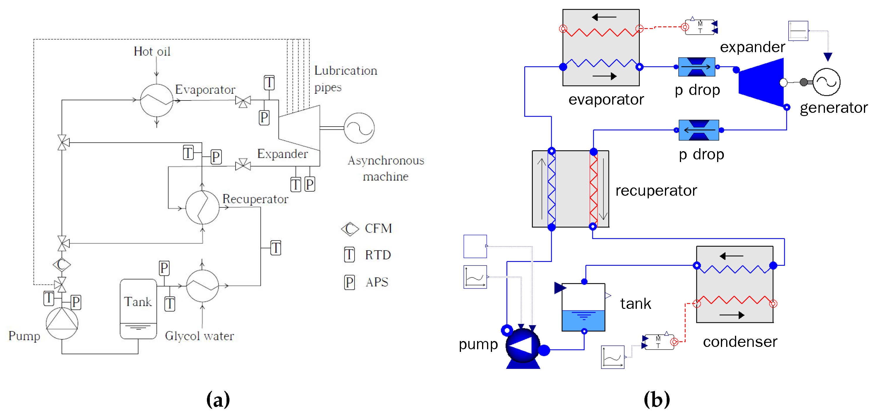
4.1. ORC Test Rig Facility

The ORC setup used to acquire the experimental data for dynamic model validation is depicted in Figure 3a. The system is equipped with a 14-stage centrifugal pump and a single screw expander with a nominal shaft power of 11 kW. The same brazed plate heat exchanger type is used for the evaporator, recuperator and condenser. SES36 is the selected working fluid. Oil is added to the cycle with a mass concentration of 3% to lubricate the rotor, while the bearings are lubricated through a by-pass pipe from the pump outlet to the expander. The thermal energy source is provided by means of an electrical boiler through which the thermal oil, Therminol66 (EASTMAN, Kingsport, TN, USA), is heated to temperatures of up to 125 °C. A proportional integral (PI) controller ensures a constant oil temperature at the inlet of the evaporator when the ORC unit undergoes transient conditions (e.g., change of ORC pump rotational speed). In the condenser, the working fluid thermal energy is absorbed by a variable glycol water flow rate, which rejects the heat to the ambient environment by means of two constant speed fans. The absolute pressure sensor (APS) and resistance temperature detectors (RTD) are placed at the inlet and at the outlet of each ORC unit component. The working fluid mass flow rate is measured by means of a Coriolis flow meter. The expander and pump are connected to two inverters, which allow controlling the rotational speed of the machines. During the experimental campaign, the evaporator was insulated with a glass wool layer. A programmable logic controller (PLC) unit allows for data acquisition and provides basic assistance features during start up and shut down. A LabView interface allows for the implementation of the advanced control strategy and data visualization. In Table 3, the measurement device characteristics are reported. For a more detailed description of the test rig and an analysis of its performance, the interested reader can refer to [26].

4.2. ORC System Modelica Model

When modeling a low-capacity power unit, since the time constants characterizing the expansion and compression processes are small compared to those of the heat exchangers, steady-state models can be used to simulate the expander and the pump components. In this work, the expansion machine is modeled by its effectiveness, expressed with a formulation proposed by [27], and the filling factor. The pump model is based on two empirical correlations, one for the effectiveness as a function of the pressure ratio and the pump speed and one for the delivered mass flow rate as a function of the pump speed. The empirical coefficients for the different performance curves have been derived based on the acquired measurements of the test unit. A more detailed description of this process together with the values of the coefficients is reported in [28]. The tank at the condenser outlet is modeled assuming thermodynamic equilibrium at all times and accounting for mass and energy accumulation. A lumped approach is applied for pressure drop modeling. Two pressure drop components are placed at the lowest vapor density part of both the low and high pressure lines accounting for laminar and turbulent phenomena. Such an approach facilitates the convergence of the numerical integration process and is valid as long as the pressure drops remain limited [23]. The recuperator and the condenser components are modeled with the FV model described in Section 2.2. The evaporator is modeled using both the FV and the MB models in order to investigate the difference between the two approaches at the system level. The computation of the thermo-physical properties of Solkatherm and water-glycol is accomplished coupling Modelica to the open-source CoolProp library [14] through the ExternalMedia package [13]. In particular, the density smooth method described in [22] is used for the Solkatherm model. The thermal oil, Therminol66, is modeled as an incompressible fluid with a model included in the ThermoCycle library, importing the incompressible fluid model of the MSL based on tables. In this work, the ORC model simulations are run using Dymola2014 (Dassault Systemes AB, Lund, Sweden) with VisualStudio2010 as the compiler. The ORC model layout is shown in Figure 3b from the Modelica-Dymola graphical user interface.

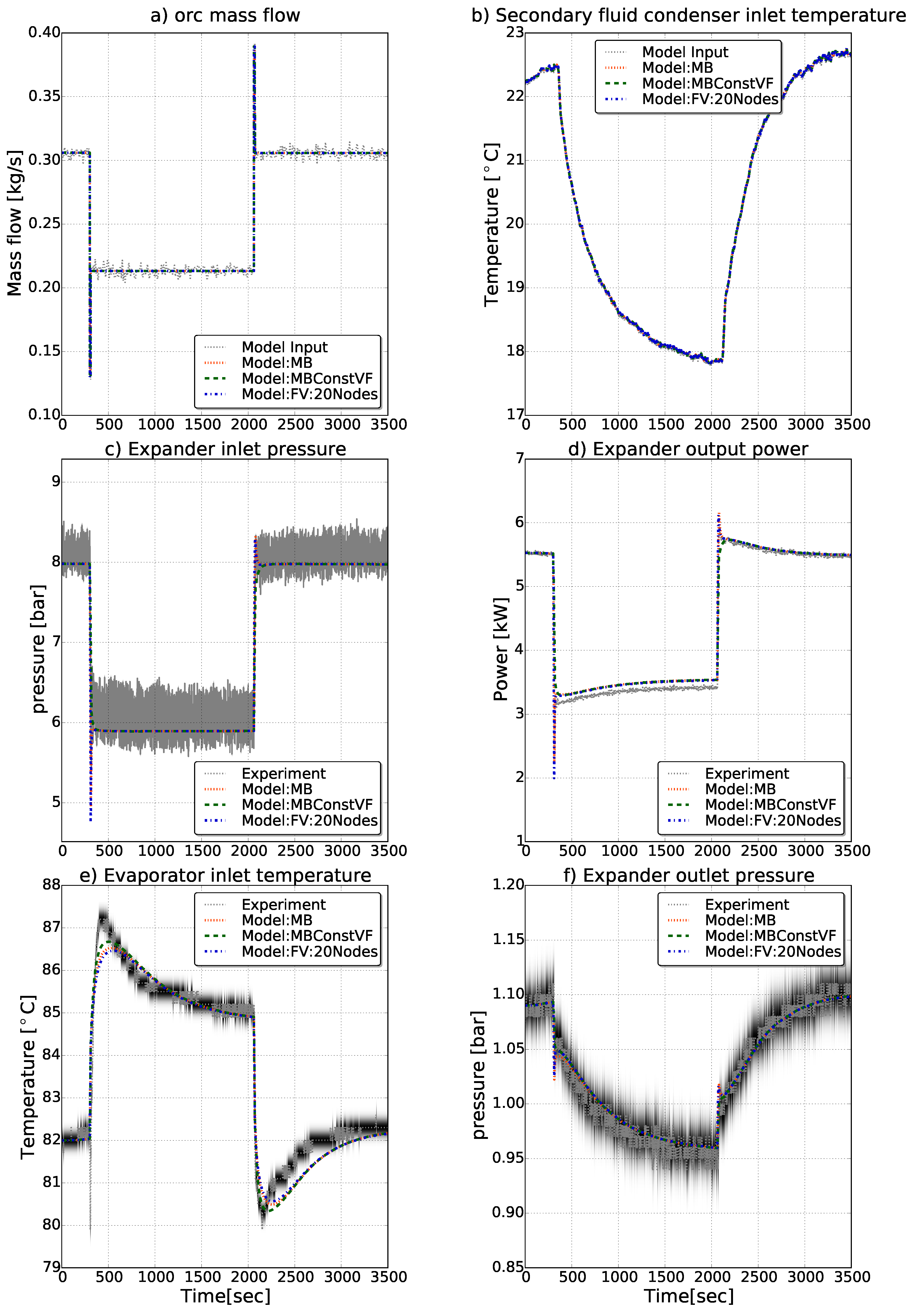
4.3. Model Validation

The transient response of the ORC unit is investigated by applying two consecutive step changes of the same magnitude to the pump rotational speed, starting from a steady-state condition. The effectiveness of the finite volume and the moving boundary model with a calculated and a constant void fraction of 0.9 is checked by replicating the pump step change experiment on the developed Modelica ORC model, using as an evaporator the finite volume and the moving boundary model. The FV evaporator model is discretized into 20 control volumes, which is revealed to be a good compromise between model accuracy and computational time, as reported in Section 4.5. The evaporator models are parametrized based on the manufacturer data sheet. The assumed-to-be constant heat exchanger coefficients values are calculated with correlations available in the literature and are slightly modified to match the experimental results.
In Figure 4, the comparison between the measurements and the simulation results is reported. Figure 4a,b shows the two dynamic inputs imposed on the model: the SES36 mass flow rate and the water-glycol temperature at the condenser inlet. As shown in Figure 4a, the SES36 mass flow rate measurement is affected by noise. To overcome this problem, the signal is smoothed out using a spline function and is used as the model input. Due to a lack of information on the cooling loop, the oscillations characterizing the measured water-glycol temperature at the condenser inlet are simulated with a spline signal and imposed as an input to the model, as shown in Figure 4b.
The downwards and upwards steps are imposed at time t = 300 s and t = 2061 s, respectively. When the pump speed is decreased/increased and the expander rotational speed is kept constant, the velocity and pressure of the fluid in the high pressure line decreases/increases. This results in a decrease/increase of density and, consequently, of the mass flow rate. Despite the symmetrical characteristic of the upwards and downwards steps imposed on the pump rotational speed, the ORC unit responses are characterized by divergent trends due to the non-linear nature of the power system. The pressure at the expander inlet and, consequently, the expander output power trends are characterized by a fast negative overshoot at time t = 300 s, as depicted in Figure 4c,d. When the pump speed is increased, an overshoot of lower amplitude is measured for the same two variables.
The measured evaporator inlet temperature trend shows a fast and negative overshoot when the pump speed is decreased at time t = 300 s, as shown in Figure 4e. A disturbance in the temperature measurement device could be identified as the reason for such a phenomena. The evaporator is characterized by a very small pinch point placed at the outlet of the working fluid side, which is related to the oversizing of the heat exchange area [26]. As a consequence, the temperature at the evaporator outlet remains fairly constant throughout the dynamic experiments and is not plotted in Figure 4.
The low pressure side is characterized by fast dynamics related to the pump speed change followed by a much slower dynamic imposed by the temperature change of the cooling fluid at the condenser inlet.
The simulation results for the three models replicate well the main dynamics characterizing the system. It is interesting to note that when the void fraction is kept constant in the MB model, MBConstFV, the response of the model is slower compared to that of the real unit. In particular, the MBConstFV model is not able to replicate the fast overshoot/undershoot that characterizes the pressure at the inlet of the expander and the expander output power when the pump speed is changed. This phenomenon is analyzed and explained in detail in Section 4.4.
In Table 4, the computational time required by the different ORC unit models to simulate is reported as a percentage of the total simulation time. The moving boundary model allows one to decrease the simulation speed by a factor of 10 while keeping a high accuracy with respect to the experimental results.

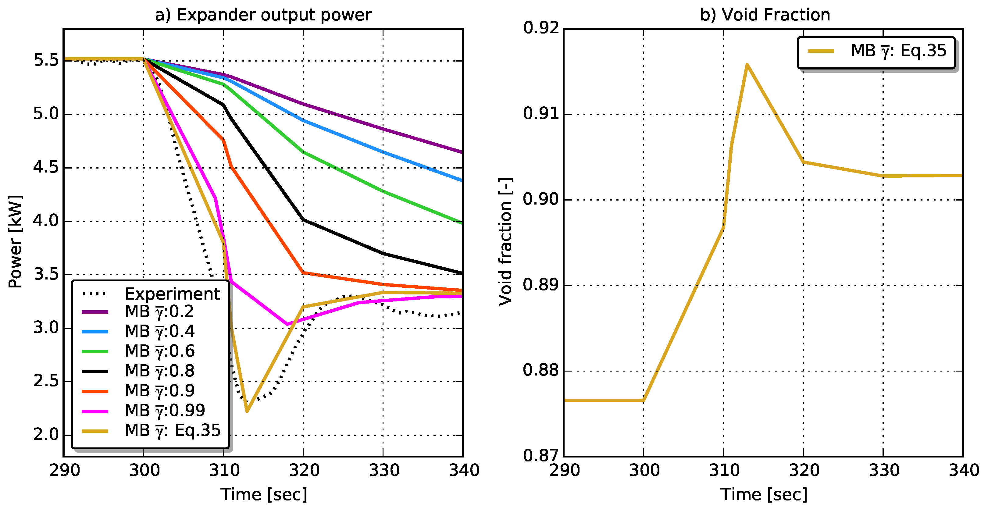
4.4. Moving Boundary: Mean Void Fraction Parametric Analysis

In order to further investigate the effect of the mean void fraction on the MB evaporator model performance, a parametric analysis is performed by replacing the endogenously-computed value of the mean void fraction, γ (see Equation (A5)), by six different constant values ranging from 0.2 to 0.99. The range upper limit is set as the highest void fraction value in the two-phase region before the fluid gets completely evaporated. The results are reported in Figure 5 for the pump speed step change downwards experiment.
In Figure 5a, the expander output power simulation results for the different MB evaporator models are compared to the experimental data. As the void fraction value increases, the simulation results get closer to the measurements. In particular, a value of 0.2 considerably overestimates the time constant, while a value of 0.99 approaches much better the experimental data. As is clearly depicted in Figure 5a, an increase of the void fraction value in the evaporator MB model corresponds to a decrease of the expander output power time constant. This can be explained by the fact that a larger void fraction value results in an increased portion of the evaporator volume filled with gas, which corresponds to a lower thermal inertia of the evaporator and, therefore, to a smaller time constant. None of the MB models with a constant void fraction are able to predict the overshoot characterizing the power output power trend. This is explained by the fact that when the mass flow decreases, the void fraction increases, as shown in Figure 5b, as the portion of the area occupied by the gas increases. As a consequence, the thermal capacity decreases, leading to faster transients. Keeping the mean void fraction constant neglects this phenomena and results in a too slow response. It also results in a poor prediction of the outlet flow rate variations during transients. To conclude, the void fraction needs to be computed analytically in order to follow the fast mass flow variation of the system, as shown in Figure 5b.

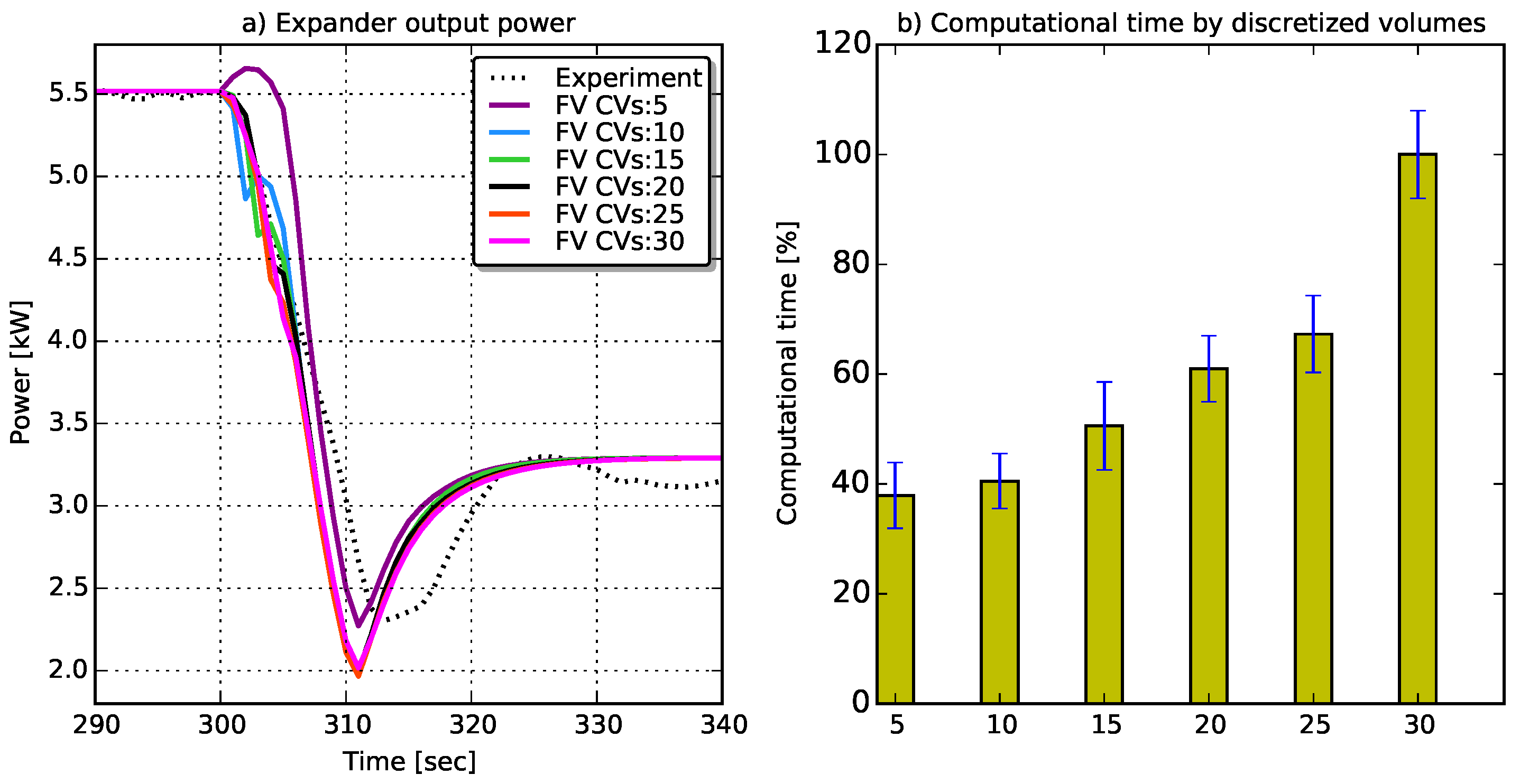
4.5. Finite Volume: Number of CVs Parametric Analysis

A parametric study to investigate the performance of the FV evaporator model with different levels of discretization is reported in this section. The number of CVs is varied in a range from five to 30. The results are displayed in Figure 6 for the pump speed step change downwards. In Figure 6a, the expander output power simulation results for different FV evaporator models are compared to the experimental data. For a number of CVs below 20, a non-physical oscillation between time t = 300 s and t = 310 s characterizes the expander output power simulation results. This phenomenon is explained by the displacement of the working fluid phase boundary from one cell to the next. This generates a numerical mass flow rate due to the discontinuity characterizing the density in the regions around the saturation lines [22]. Increasing the number of CVs allows one to reduce the magnitude of this phenomenon. For a level of discretization above 20 CVs, negligible differences in the simulation results are registered, while the computational time of the models increases significantly, as shown in Figure 6b. This analysis allows one to identify a level of discretization of 20 CVs as a good compromise between accuracy and simulation speed for this specific simulation.

5. Conclusions

In this work, a comparison of the finite volume and the moving boundary approaches to simulate the dynamics characterizing an evaporator is proposed. An integrity and stability test for each approach has been performed, taking as the benchmarking indicator the simulation speed, the conservation of mass and energy and the mean percentage relative error, ε ¯ , for outlet enthalpy and mass flow rate with respect to a 100 CVs finite volume. In order to assess the two modeling approaches’ performances when integrated at a system level, the FV and the MB models are used in the Modelica model of a small 11 kWel ORC power unit to simulate the evaporator component. The transient responses of the models are compared against experimental results. Furthermore, two parametric analyzes are performed to analyze in detail the effect of varying the void fraction value in the MB evaporator model and of varying the level of discretization in the FV one. The main outcomes of this study are summarized below:
  • The integrity test results allow one to conclude that both the MB and FV approaches are well suited for dynamic modeling of two-phase heat exchanger components being characterized by a low error on the total conservation of energy and mass.
  • The MB proves much faster compared to the 100 CVs FV model with a computational time three orders of magnitude lower. These results are in line with the ones presented in [21,29].
  • The comparison against experimental transients of a small 11 kWel ORC power unit demonstrates that both the FV and the MB with an analytically calculated void fraction approaches are suitable for the dynamic modeling of the evaporator when integrated at the system level. The moving boundary model allows one to decrease significantly the simulation speed while keeping a good accuracy with the experimental data.
  • In the proposed comparison, the assumption of homogeneous two-phase flow does not lead to inaccurate estimation of the time constant characterizing the system and can be considered appropriate for the modeling of a small capacity thermal power unit.
  • Assuming a constant void fraction in the MB approach results in an overestimation of the dynamics (i.e., leading to slower response times), making it unsuitable for modeling a small capacity heat exchanger. From the proposed parametric analysis, it is clear that the average void fraction is inversely proportional to the time constant characterizing the evaporator model.
  • When using an FV model, the level of discretization needs to be accurately selected. In the case of a small-scale ORC unit using plate heat exchangers, a minimum number of 20 nodes is recommended to avoid numerical inconsistency in the simulation results.
  • Despite what is stated in the literature [21], the two modeling formulations are found to have a comparable level of robustness, i.e., both the FV and MB models are able to smoothly run the performed simulations. A wider range of simulation tests (e.g., start-up and shut-down of vapor compression cycles) is deemed necessary to further investigate the robustness of the two modeling approaches.
The proposed MB and FV models together with the test cases were released as open-source and are available in the latest version of the ThermoCycle library.
In future works, an experimental campaign focusing on the specific dynamics characterizing the evaporator and condenser components is planned. The recorded data will be used to perform a more detailed validation of the FV and MB models for low-capacity plate heat exchangers.

Acknowledgments

The results presented in this paper have been obtained within the frame of the IWT SBO-110006 project The Next Generation Organic Rankine Cycles (http://www.orcnext.be/), funded by the Institute for the Promotion and Innovation by Science and Technology in Flanders. This financial support is gratefully acknowledged.

Author Contributions

Adriano Desideri, Jorrit Wronski and Sylvain Quoilin conceived of and designed the finite volume and the moving boundary model. Adriano Desideri and Sergei Gusev performed the experiments. Martijn van den Broek was in charge of the experimental test rig. Adriano Desideri and Bertrand Deschesne analyzed the simulation data. Vincent Lemort contributed to the development of the overall work. Adriano Desideri wrote the paper.

Conflicts of Interest

The authors declare no conflict of interest.

Abbreviations

The following abbreviations are used in this manuscript:
ORC
Organic Rankine cycle
APS
Absolute pressure sensor
RTD
Resistance temperature detector
CFM
Coriolis flow meter
FV
Finite volume
MB
Moving boundary
CV
Control volume
MSL
Modelica Standard library

Appendix A

In this section, the process to derive the mean void fraction is reported. The regularly-used quantities at the phase boundaries at constant pressure are denoted with ′ for the liquid phase and ″ for the vapor phase. The area average void fraction, which is the most adopted definition of the void fraction γ [24], and the static quality are defined as shown in Equations (A1) and (A2).
γ = A A
x = M M
where M is the mass of vapor in the two-phase volume, M is the total mass flow of the fluid and A and A are the pipe cross-section occupied by the vapor and the total cross-section, respectively. From Equations (A1) and (A2), it follows that:
x = γ V ρ V ( γ ρ + ( 1 γ ) ρ ) = γ ρ ( γ ρ + ( 1 γ ) ρ )
Rearranging Equation (A3), the void fraction can be expressed as:
γ ( p , h ) = x ρ x ρ + 1 x ρ
Defining the enthalpy at the boundary of the two-phase control volume as h a and h b , the average void fraction, γ ¯ , can be computed integrating Equation (A4) over the enthalpy range Δ h = h b h a as a function of pressure and the two boundary enthalpies:
γ ¯ ( p , h a , h b ) = h a h b γ ( p , h ) d h = ρ 2 ( h a h b ) + ρ ρ h b h a + ( h h ) Γ ( h a ) Γ ( h b ) h a h b ρ ρ 2
with Γ ( h ) = ρ ( h h ) + ρ ( h h )

Appendix B

In this section, the formulation of the average void fraction partial derivatives adopted in the two-phase cell of the moving boundary model are reported. The average void fraction time derivative is expressed as:
d γ ¯ d t = + γ ¯ p d p d t + γ ¯ h a d h a d t + γ ¯ h b d h b d t
The partial derivative with respect to pressure is reported in Equation (A8).
γ ¯ p = + d ρ d p Δ h a b Δ ρ t p 2 Δ h a b ρ + ρ Δ h a b , t p 2 ρ d ρ d p d ρ d p Δ h a b Δ ρ t p 3 Δ h a b ρ + ρ Δ h a b , t p + ρ Δ h a b Δ ρ t p 2 Δ h a b d ρ d p + d ρ d p Δ h a b , t p + ρ d h d p d h d p ln G + Δ h t p Γ ( h a ) Θ ( h a ) G Θ ( h b )
The partial derivatives with respect to h a and h b are reported in Equations (A9) and (A10), respectively
γ ¯ h a = ρ Δ h a b 2 Δ ρ t p 2 Δ h a b ρ + ρ Δ h a b , t p + ρ Δ h a b Δ ρ t p 2 + ρ + ρ 1 + Δ h t p Δ ρ t p Γ ( h a )
γ ¯ h b = + ρ Δ h a b 2 Δ ρ t p 2 Δ h a b ρ + ρ Δ h a b , t p + ρ Δ h a b Δ ρ t p 2 ρ + ρ + 1 Δ h t p Δ ρ t p Γ ( h b )
with : Δ h t p = h h , Δ ρ t p = ρ ρ , Δ h a b = h a h b , Θ ( h ) = h h d ρ d p ρ d h d p + h h d ρ d p + ρ d h d p , Δ h a b , t p = Δ h a b + Δ h t p ln G , and G = Γ ( h a ) / Γ ( h b )
with Γ ( h ) as defined in Equation (A6).

References

  1. Colonna, P.; van Putten, H. Dynamic modeling of steam power cycles: Part I—Modeling paradigm and validation. Appl. Therm. Eng. 2007, 27, 467–480. [Google Scholar] [CrossRef]
  2. Mattsson, S.; Elmqvist, H. Modelica—An international effort to design the next generation modeling language. In Proceedings of the 7th IFAC Symposium on Computer Aided Control Systems Design, Gent, Belgium, 28–30 April 1997.
  3. Dymola, Modelon. Available online: http://www.modelon.com/products/dymola/ (accessed on 14 March 2016).
  4. OpenModelica. Available online: https://openmodelica.org/ (accessed on 14 March 2016).
  5. Mehrmann, V.; Wunderlich, L. Hybrid systems of differential-algebraic equations—Analysis and numerical solution. J. Process Control 2009, 19, 1218–1228. [Google Scholar] [CrossRef]
  6. Casella, F.; Leva, A. Object-oriented modelling and simulation of power plants with Modelica. In Proceedings of the 44th IEEE Conference on Decision and Control, and the European Control Conference, Plaza de España Seville, Spain, 12–15 December 2005.
  7. Tummescheit, H.; Eborn, J.; Wagner, F.J. Development of a Modelica base library for modeling of Thermo-Hydraulic systems. In Proceedings of the Modelica Workshop, Lund, Sweden, 23–24 October 2000.
  8. El Hefni, B. Dynamic modeling of concentrated solar power plants with the ThermoSysPro library (Parabolic Trough collectors, Fresnel reflector and Solar-Hybrid). Energy Procedia 2013, 49, 1127–1137. [Google Scholar] [CrossRef]
  9. Thermal Power Library, Modelon. Available online: http://www.modelon.com/products/modelica-libraries/thermal-power-library/ (accessed on 14 March 2016).
  10. Casella, F.; Leva, A. Modelica open library for power plant simulation: Design and experimental validation. In Proceedings of the 3rd International Modelica Conference, Linköping, Sweden, 3–4 November 2003; pp. 41–50.
  11. TIL Suite, TLK-ThermoGmbH. Available online: http://www.tlk-thermo.com/index.php/en/software-products/til-suite (accessed on 14 March 2016).
  12. Wetter, M. Modelica library for building heating, ventilation and air-conditioning systems. 2009. [Google Scholar] [CrossRef]
  13. Quoilin, S.; Desideri, A.; Wronski, J.; Bell, I.H.; Lemort, V. ThermoCycle: A Modelica library for the simulation of thermodynamic systems. In Proceedings of the 10th International Modelica Conference, Lund, Sweden, 10–12 March 2014.
  14. Bell, I.; Wronski, J.; Quoilin, S.; Lemort, V. Pure- and Pseudo-pure fluid thermophysical property evaluation and the open-source Thermophysical Property Library CoolProp. Ind. Eng. Chem. Res. 2014, 53, 2498–2508. [Google Scholar] [CrossRef] [PubMed] [Green Version]
  15. Bendapudi, S.; Braun, J.; Groll, E.; Eckhard, A. Dynamic model of a centrifugal chiller system–Model development, numerical study and validation. ASHRAE Trans. 2005, 111, 132. [Google Scholar]
  16. Dhar, M.; Soedel, W. Transient analysis of a vapor compression refrigeration system. In Proceedings of the XV International Congress of Refrigeration, Venice, Italy, 23–29 September 1979.
  17. MacArtur, J.; Grald, E. Prediction of cyclic heat pump performance with a fully distributed model and a comparison with experimental data. ASHRAE Trans. 1987, 93, 1159–1178. [Google Scholar]
  18. Bendapudi, S. A Literature Review of Dynamic Models of Vapor Compression Equipment; Technical Report; Herrick Laboratories, Purdue University: West Lafayette, IN, USA, 2002. [Google Scholar]
  19. Bendapudi, S. Development and Validation of a Mechanistic Dynamic Model for a Vapor Compression Centrifugal Liquid Chiller; Technical Report; Herrick Laboratories, Purdue University: West Lafayette, IN, USA, 2002. [Google Scholar]
  20. Bonilla, J.; Dormido, S.; Cellier, F.E. Switching moving boundary models for two-phase flow evaporators and condensers. Commun. Nonlinear Sci. Numer. Simul. 2015, 20, 743–768. [Google Scholar] [CrossRef]
  21. Bendapudi, S.; Braun, J.E.; Groll, E.A. A comparison of moving-boundary and finite-volume formulations for transients in centrifugal chillers. Int. J. Refrig. 2008, 31, 1437–1452. [Google Scholar] [CrossRef]
  22. Quoilin, S.; Bell, I.H.; Desideri, A.; Dewallef, P.; Lemort, V. Methods to increase the robustness of finite-volume flow models in Thermodynamic systems. Energies 2014, 7, 1621–1640. [Google Scholar] [CrossRef]
  23. Quoilin, S. Sustainable Energy Conversion Through the Use of Organic Rankine Cycles for Waste Heat Recovery and Solar Applications. Ph.D. Thesis, University of Liege, Liege, Belgium, October 2011. [Google Scholar]
  24. Jensen, J.M. Dynamic Modeling of Thermo-Fluid Systems. Ph.D. Thesis, Technical University of Denmark, Lyngby, Denmark, 2003. [Google Scholar]
  25. Petzold, L.R. A Description of DASSL: A Differential/Algebraic System Solver; Technical Report, Sandia Report SAND82-8637; IMACS World Congress: Montreal, QC, Canada, 1982. [Google Scholar]
  26. Desideri, A.; Sergei, G.; van den Broek, M.; Lemort, V.; Quoilin, S. Experimental comparison of organic fluids for low temperature ORC (organic Rankine cycle) systems for waste heat recovery applications. Energy 2016, 97, 460–469. [Google Scholar] [CrossRef]
  27. Declaye, S.; Quoilin, S.; Guillaume, L.; Lemort, V. Experimental study on an open-drive scroll expander integrated into an ORC (organic Rankine cycle) system with R245fa as working fluid. Energy 2013, 55, 173–183. [Google Scholar] [CrossRef]
  28. Desideri, A.; van den Broek, M.; Gusev, S.; Lemort, V.; Quoilin, S. Experimental campaign and modeling of a low-capacity waste heat recovery system based on a single screw expander. In Proceedings of the 22nd International Compressor Engineering Conference, Purdue, West Lafayette, IN, USA, 14–17 July 2014.
  29. Grald, E.W.; MacArthur, J.W. A moving-boundary formulation for modeling time-dependent two-phase flows. Int. J. Heat Fluid Flow 1992, 13, 266–272. [Google Scholar] [CrossRef]
Figure 1. Representation of the finite volume (a) and the moving boundary (b) heat exchanger from the Dymola graphical user iterface (GUI).
Energies 09 00339 g001
Figure 2. Temperature profiles of the finite volume (a) and the moving boundary (b) evaporator models as they are assumed by the application of Newton’s law of cooling to solve the heat transfer problem. Each segment corresponds to one control volume.
Energies 09 00339 g002
Figure 3. Process flow diagram of the ORC with the sensors’ position (a) and the ORC system model from the Modelica-Dymola GUI (b). CFM, Coriolis flow meter; RTD, resistance temperature detector; APS, absolute pressure sensor.
Energies 09 00339 g003
Figure 4. Downward-upward 5-Hz step change to the pump rotational speed.
Energies 09 00339 g004
Figure 5. Results of the void fraction parametric analysis for the MB evaporator model. (a) Expander output power for different void fraction values in the MB evaporator model. (b) Void fraction trend in the MB evaporator model when analytically computed.
Energies 09 00339 g005
Figure 6. Results of the number of control volumes (CVs) parametric analysis for the FV evaporator model. (a) Expander output power as predicted by the finite volume model for different discretization levels. (b) Computational time for the different discretization levels.
Energies 09 00339 g006
Table 1. Specific boundary enthalpy derivative depending on the heat transfer and control volume. HE, heat exchanger.
HE RegionEvaporatorCondenser
Sub-cooled
d h b d t = h l p d p d t
d h a d t = h l p d p d t
Super-heated
d h a d t = h v p d p d t
d h b d t = h v p d p d t
Table 2. Benchmarking indicators for the integrity and accuracy test for the moving boundary and the finite volume models. MBConstVF, moving boundary with the constant void fraction; FV, finite volume.
ModelMBConstVFMBFV 10 CVsFV 20 CVsFV 40 CVsFV 100 CVs
ϵ mass (%)2.33 × 10−131.08 × 10−121.72 × 10−136.33 × 10−133.06 × 10−141.01 × 10⁻¹²
ϵ ener (%)6.67 × 10−129.51 × 10−125.28 × 10−122.89 × 10−124.64 × 10−121.04 × 10⁻¹²
ε ¯   h ex (%)0.550.693.161.060.310.0
ε ¯   m ˙ ex (%)3.881.405.521.850.530.0
Time (s)0.650.732.8913.734.8147
Table 3. Range and precision of the measurement devices installed on the ORC test rig. k: coverage factor.
VariableDevice TypeRangeUncertainty (k = 2)
m ˙ CFM0 to 1.8 kg·s−1±0.09%
T (ORC)RTD−50 to 300 °C±0.2 K
T (heat sink)RTD0 to 150 °C±0.2 K
T (heat source)RTD30 to 350 °C±0.2 K
pAPS0 to 16 bar±0.016 bar
W ˙ el Wattmeter0 to 34.6 kW±0.1%
Table 4. CPU time for integration as the percentage of the total simulation time.
ModelCPU-Time (%)
ORC unit model with FV13.5
ORC unit model with MB2.45
ORC unit model with MBConstFV2.4

