
Numerical Evaluation and Optimization of Multiple Hydraulically Fractured Parameters Using a Flow-Stress-Damage Coupled Approach

Abstract
:
1. Introduction
2. Hydraulic Fracturing Model Setup
2.1. Brief Description of the Numerical Model
- (1)
- the RFPA-Flow code can simulate the non-linear deformation of a quasi-brittle behavior by introducing the heterogeneity of rock properties into the model, with an ideal brittle constitutive law for the local material;
- (2)
- by introducing a reduction of material parameters after element failure, the RFPA code can simulate strain-softening and discontinuous mechanics problems in a continuum mechanics mode.
2.2. Realistic Failure Process Analysis-Flow Model Setup
3. Multiparameter Optimization
3.1. D-Optimal Design for Response Surface Methodology
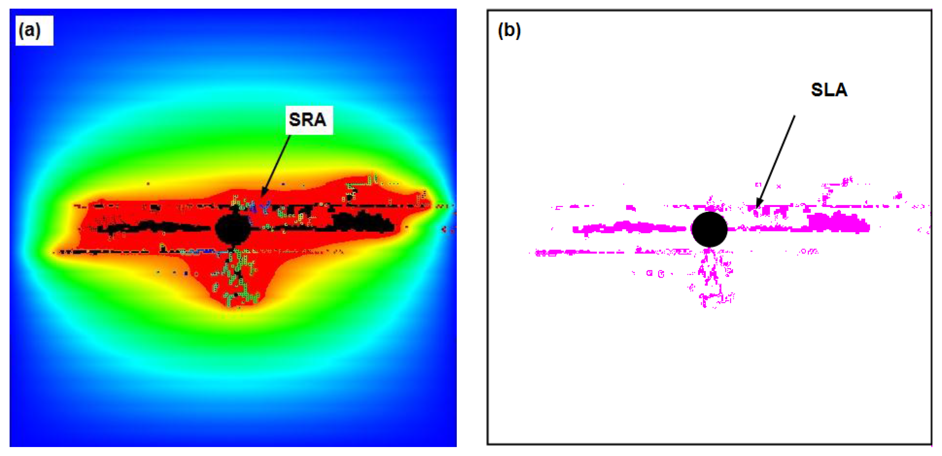
- (1)
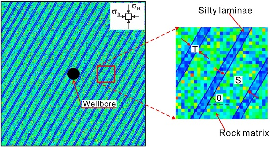
- SRA: defined as the interaction area of hydraulic fractures and silty laminae that has experienced a fluid pressure increase due to injection;
- (2)
- SLA: defined as the area of silty laminae that has been damage during hydraulic fracturing.
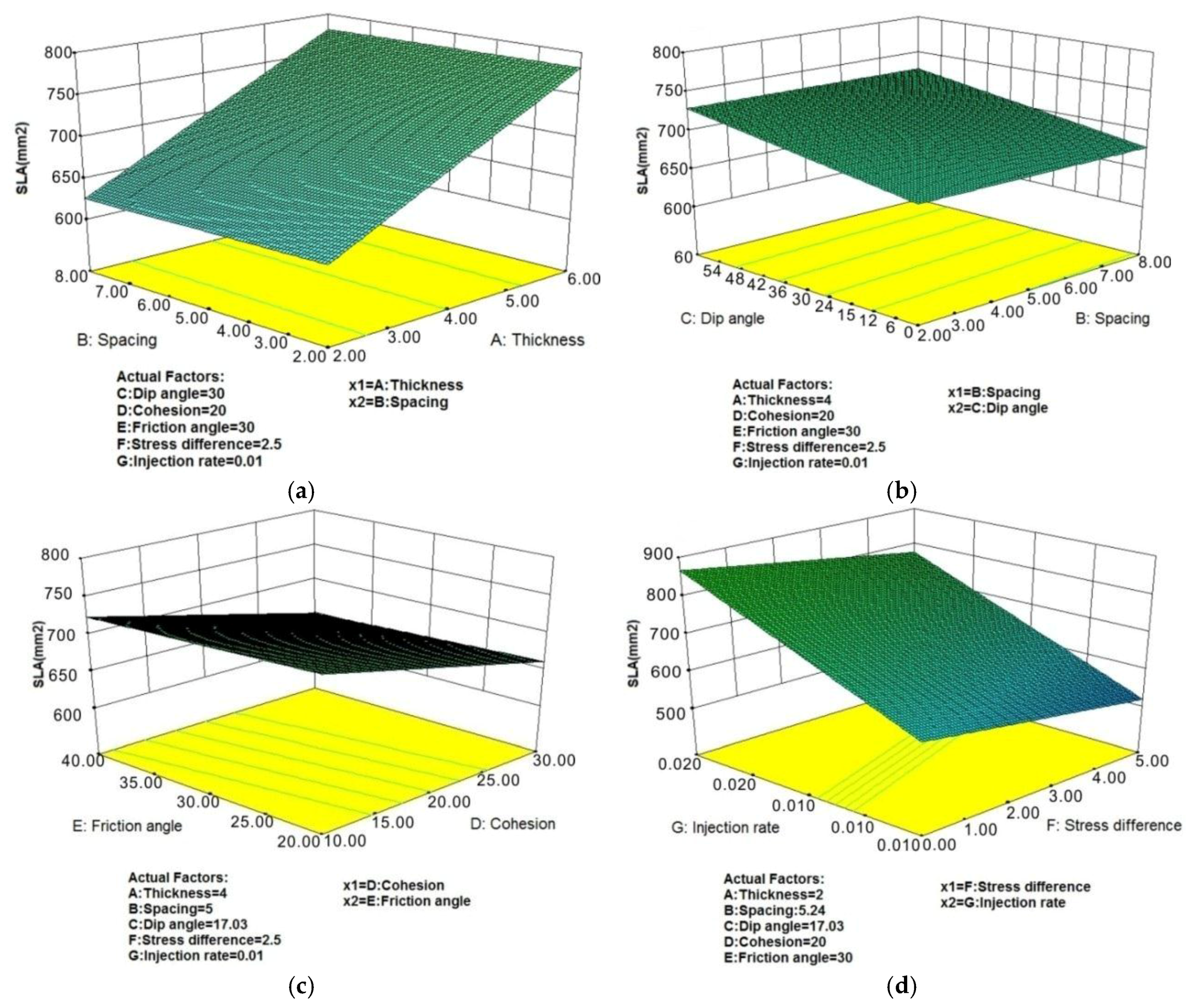
3.2. Response Surface MethodologyModel Analysis
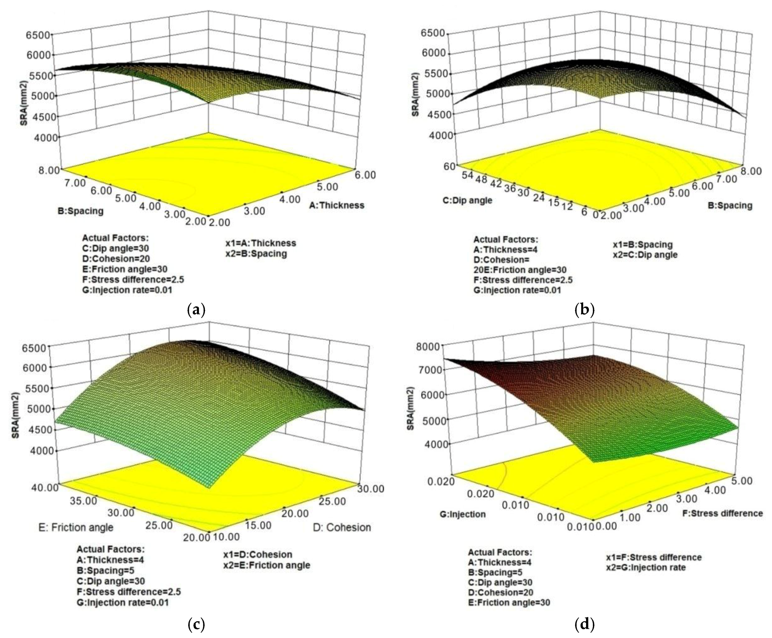
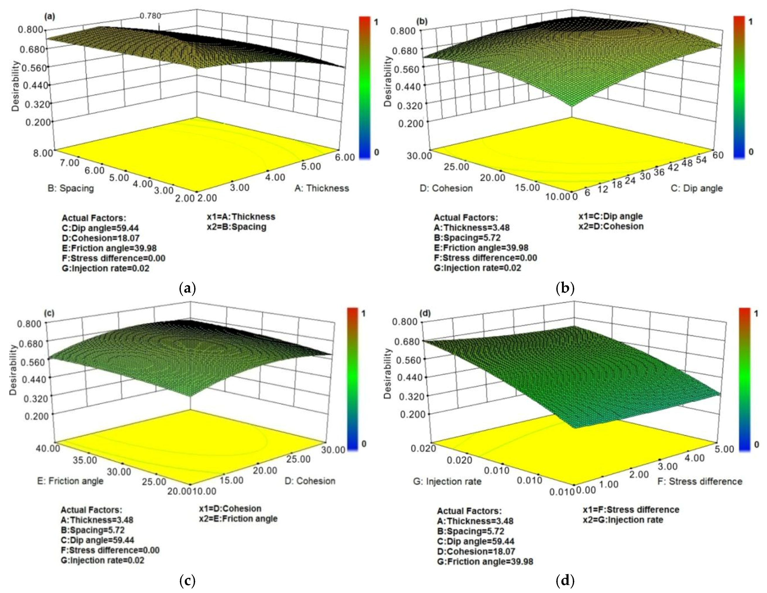
3.3. Stimulated Area Optimization
3.4. Discussion
4. Conclusions
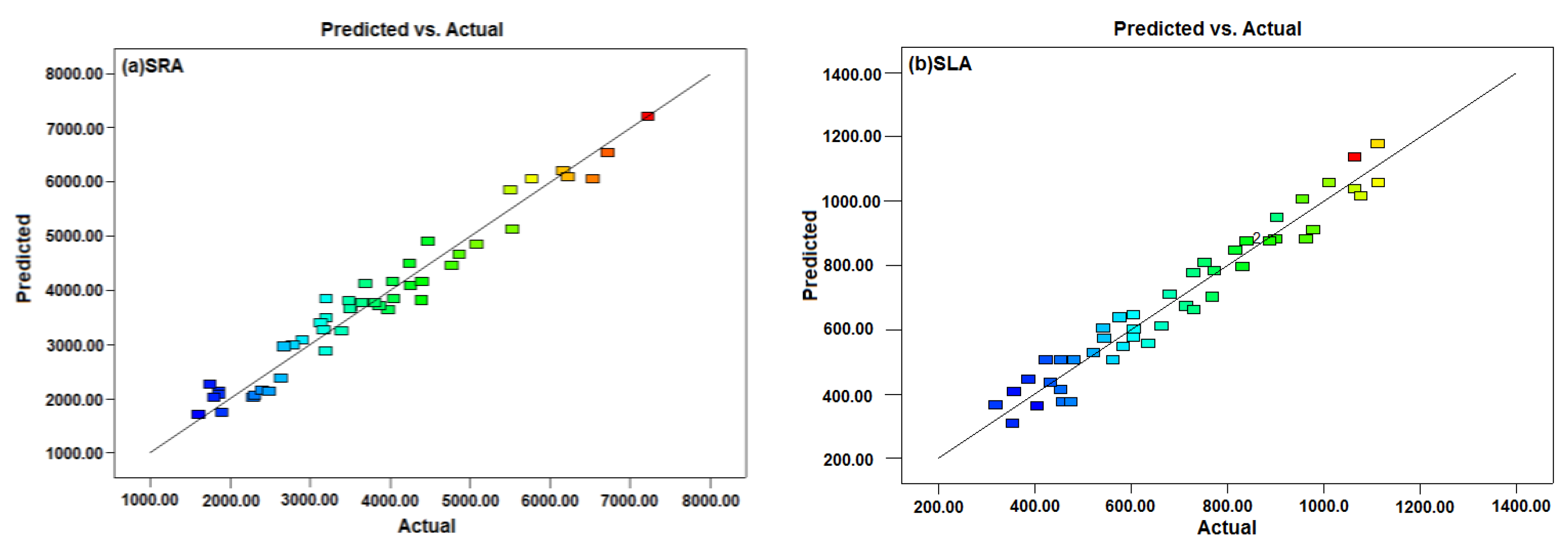
- (1)
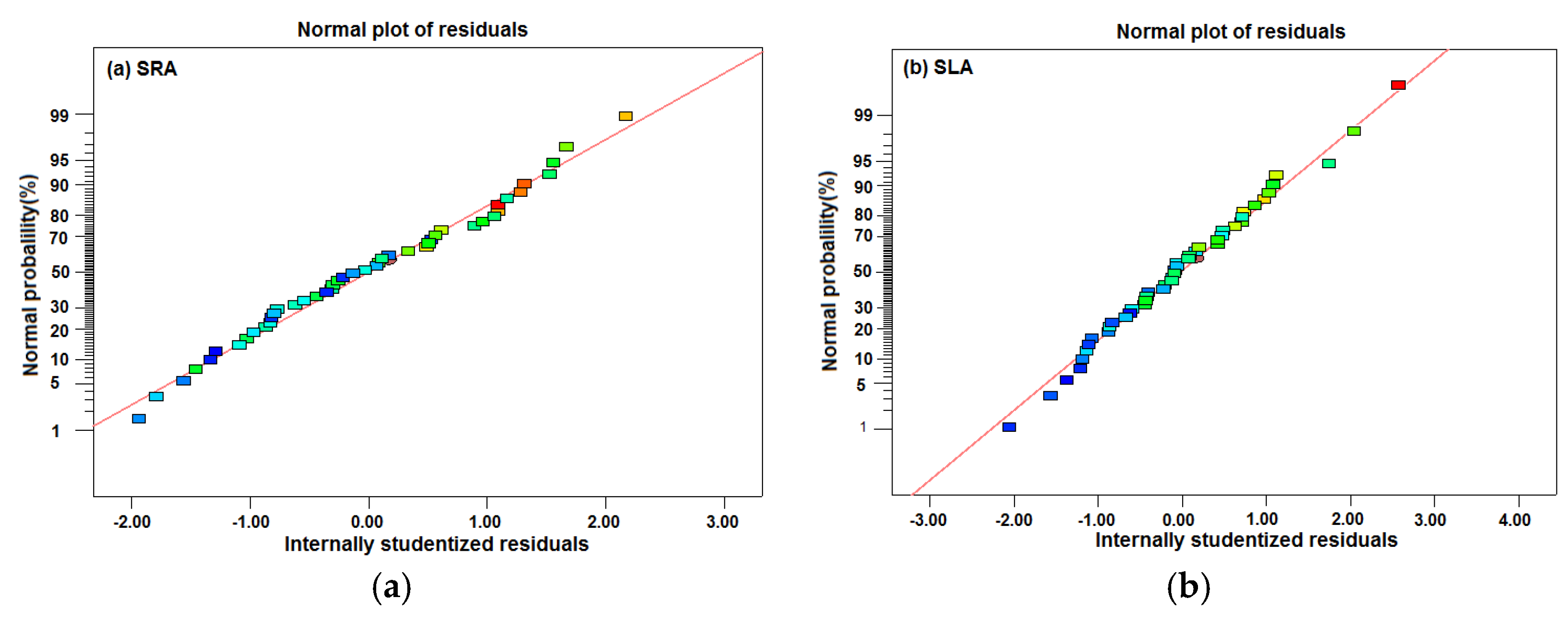
- The proposed approach is practical and efficient for the design and optimization of hydraulic fracturing multi-parameters. SRA and SLA response surface models givereliable predicted values compared with the actual values of SRA and SLA;
- (2)
- By the RSM optimization, the optimal design combinations for silty laminae shale are obtained. Among the optimal projects, IR is a positive factor to increase SRA and SLA; dip angle of laminae is about 60° when SRA and SLA reach the maximum for all the optimal projections;
- (3)
- The thickness factor is sensitive to both SRA and SLA. Silty laminae contains plenty of free gas and solution gas, and with the increase of thickness, the free gas recovery improves. However, due to the strong leak-off characteristics of silty laminae, the factor of thickness is a negative factor for the overall stimulated area. The influence of mechanical properties is oppositein SRA compared to SLA, with lower mechanical strength, silty laminae is prone to damage and failure; the injected fluid is difficult to generate hydraulic fractures, which reduces the interaction between hydraulic fractures and silty laminae;
- (4)
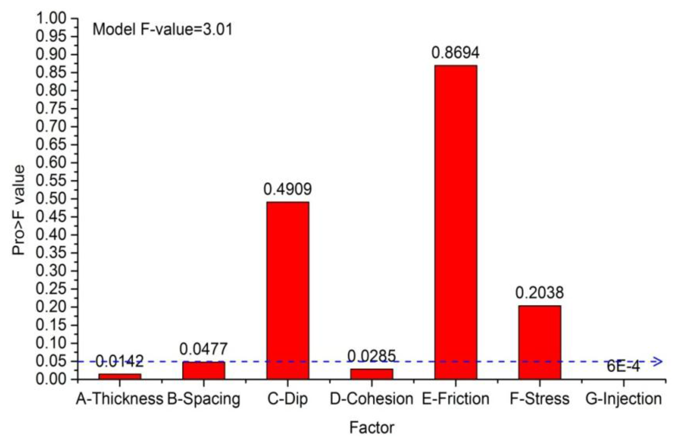
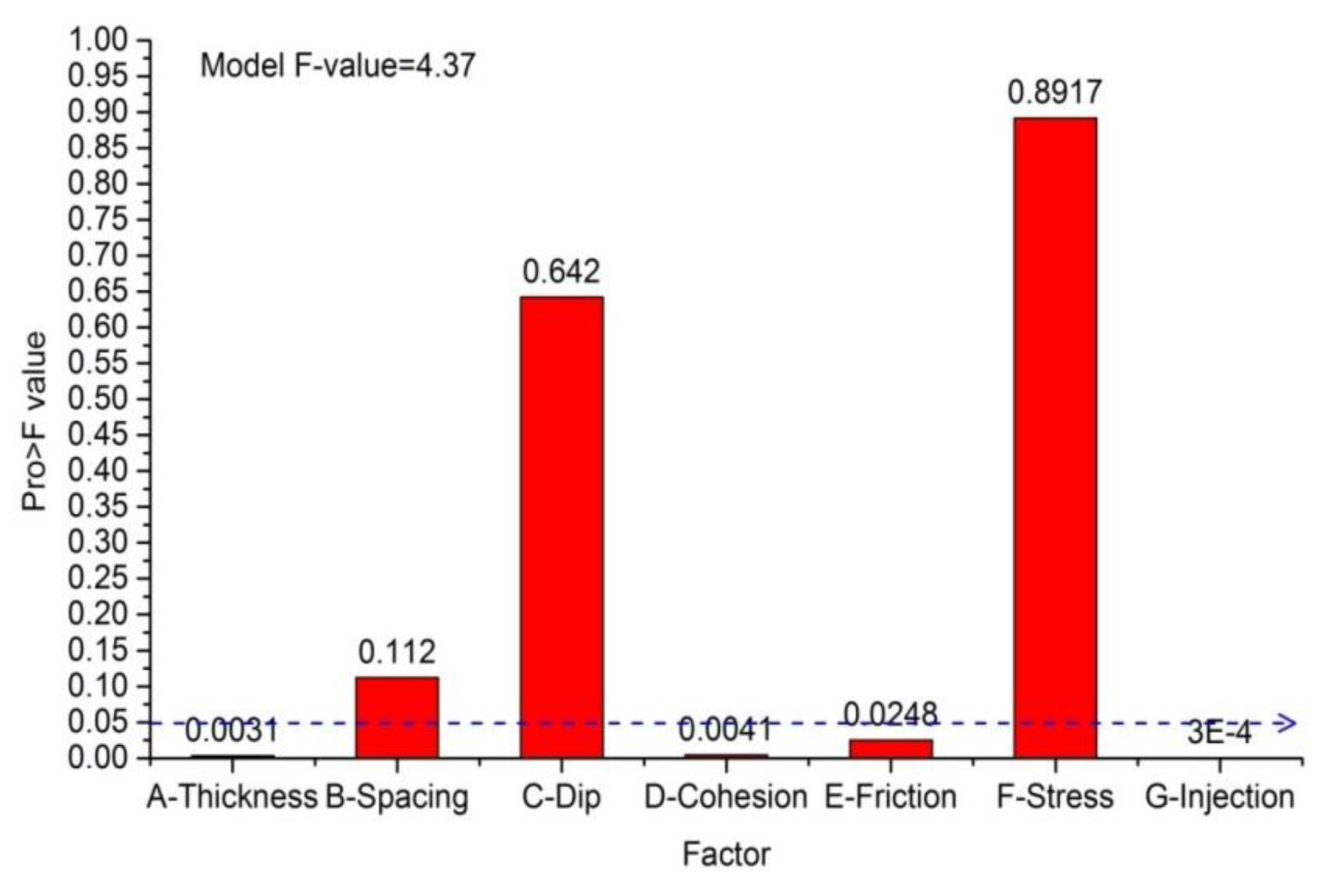
- The influential order of the studied factors to SRA is: G-IR > A-thickness > D-cohesion > E-friction angle > C-dip angle > B-spacing > F-SD. And the influential order to SLA is: G-IR > A-thickness > D-cohesion> B-spacing > F-SD > C-dipangle > E-friction angle. Factors of laminae thickness, cohesion, and IR are the most significant factors for both SRA and SLA.
Acknowledgments
Author Contributions
Conflicts of Interest
References
- Liu, Q.Y.; Jin, Z.J.; Wang, Y.; Han, P.L.; Tao, Y.; Wang, Q.C.; Ren, Z.L.; Li, W.H. Gas filling pattern in Paleozoic marine carbonate reservoir of Ordos Basin. Acta Petrol. Sin. 2012, 28, 847–858. [Google Scholar]
- Tang, X.; Zhang, J.; Shan, Y.; Xiong, J. Upper Paleozoic coal measures and unconventional natural gas systems of the Ordos Basin. China Geosci. Front. 2012, 3, 863–873. [Google Scholar] [CrossRef]
- Luo, P.; Ji, L.M. Reservoir characteristics and potential evalution of continental shale gas. Nat. Gas Geosci. 2013, 24, 1060–1068. [Google Scholar]
- Tang, X.; Zhang, J.C.; Wang, X.Z.; Yu, B.S.; Ding, W.L. Shale characteristics in the southeastern Ordos Basin, China: Implications for hydrocarbon accumulation conditions and the potential of continental shales. Int. J. Coal. Geol. 2014, 128, 32–46. [Google Scholar] [CrossRef]
- Chen, Q.H. The Study on the Sedimentary System and Stratigraphic Sequence of Trassic Yanchang Formation in the Southern Part of the Ordos Basin. Master’s Thesis, The Northwest University, Xi’an, China, 2004. [Google Scholar]
- Guo, Y.Q. Research on Reservoir Microscopic Characteristic of Yanchang Formation in Fuxian Exploration of the Odros Basin. Ph.D. Thesis, Northwest University, Xi’an, China, 2006. [Google Scholar]
- Yang, H. Deposition System and Accumulation Research of Yanchang Formation in Triassic, Ordos Basin. Ph.D. Thesis, Chengdu University of Technology, Chengdu, China, 2004. [Google Scholar]
- Zhang, D.F. The Research of Sedimentary System of the Jurassic Yangchang Formation in the South of the Slope of Shanbei. Master’s Thesis, Northwest University, Xi’an, China, 2006. [Google Scholar]
- Dong, G.L. The Evaluation of Chang7 Shale Gas Reservoir Characteristicsof Yanchang Formation in Zhenyuan and Jingchuan Area. Master’s Thesis, Chengdu University of Technology, Chengdu, China, 2012. [Google Scholar]
- Lei, Y.H.; Luo, X.R.; Wang, X.Z.; Zhang, L.X.; Jiang, C.F.; Yang, W.; Yu, Y.X.; Cheng, M.; Zhang, L.K. Characteristics of silty laminae in Zhangjiatan Shale of southeastern Ordos Basin, China: Implications for shale gas formation. AAPG Bull. 2015, 99, 661–687. [Google Scholar] [CrossRef]
- Curtis, J.B. Fractured shale-gas systems. AAPG Bull. 2002, 86, 1921–1938. [Google Scholar]
- Kemp, A.E.S. Laminated sediments as palaeo-indicators. Geol. Soc. Lond. Spec. Publ. 1996, 116. [Google Scholar] [CrossRef]
- Schieber, J. Common themes in the formation and preservation of porosity in shales and mudstones: Illustrated with examples across the Phanerozoic. In Proceedings of the Society of Petroleum Engineers Unconventional Gas Conference, Pittsburgh, PA, USA, 23–25 February 2010. [CrossRef]
- Anderson, R.Y. Seasonal sedimentation: A framework for reconstructing climatic and environmenta change. Geol. Soc. London Spec. Publ. 1996, 166, 1–15. [Google Scholar] [CrossRef]
- O’Brien, N.R. Shale lamination and sedimentary processes. Geol. Soc. Lond. Spec. Publ. 1996, 116, 23–36. [Google Scholar] [CrossRef]
- Reineck, H.E.; Singh, I.B. Genesis of laminated sand and graded rhythmites in storm-sand layers of shelf mud. Sedimentology 2006, 18, 123–128. [Google Scholar] [CrossRef]
- Sutton, S.J.; Ethridge, F.G.; Almon, W.R.; Dawson, W.C.; Edwards, K.K. Textural and sequence-stratigraphic controls on sealing capacity of Lower and Upper Cretaceous shales, Denver basin, Colorado. AAPG Bull. 2004, 88, 1185–1206. [Google Scholar] [CrossRef]
- Hammes, U.; Hamlin, H.S.; Ewing, T.E. Geologic analysis of the Upper Jurassic Haynesville shale in east Texas and west Louisiana. AAPG Bull. 2011, 95, 1643–1666. [Google Scholar] [CrossRef]
- Li, Y.; Han, X.; Niu, Z.Z. Geology Characteristics of Chang-7 Reservoir of Yanchang Formationin Xiasiwan Oil field. Northwest. Geol. 2014, 47, 249–254. [Google Scholar]
- Zeng, W.T.; Zhang, J.C.; Ding, W.L. The Gas Content of Continental Yanchang Shaleand Its Main Controlling Factors: A Case Study of Liuping-171 Well in Ordos Basin. Nat. Gas Geosci. 2014, 25, 291–301. [Google Scholar]
- Liu, X.J.; Xiong, J.; Liang, L.X. Investigation of pore structure and fractal characteristics of organic-rich Yanchang formation shale in central China by nitrogen adsorption/desorption analysis. J. Nat. Gas. Sci. Eng. 2015, 22, 62–67. [Google Scholar] [CrossRef]
- Schmoker, J.W. Use of Formation-Density Logs to Determine Organic-Carbon Content in Devonian Shales of the Western Appalachian Basin and an Additional Example Based on the Bakken Formation of the Williston Basin; Petroleum Geology of the Devonian and Mississippian Black Shale of Eastern North America, US Geological Survey Bulletin: London, UK, 1993; Volume 23, pp. 1–14.
- Davies, D.K.; Bryant, W.R.; Vessell, R.K.; Burkett, P.J. Porosities, Permeabilities and Microfabrics of Devonian Shales; Springer-Verlag: New York, NY, USA, 1991; pp. 109–119. [Google Scholar]
- Rabczuk, T.; Zi, G.; Bordas, S.; Nguyen-Xuan, H.A. A simple and robust three-dimensional cracking-particle method without enrichment. Comput. Methods Appl. Mech. 2010, 199, 2437–2455. [Google Scholar] [CrossRef]
- Rabczuk, T.; Belytschko, T. Cracking particles: A simplified meshfree method for arbitrary evolving cracks. Int. J. Numer. Methods Eng. 2004, 61, 2316–2343. [Google Scholar] [CrossRef]
- Zhuang, X.; Augarde, C.E.; Mathisen, K.M. Fracture modeling using meshless methods and level sets in 3D: Framework and modeling. Int. J. Numer. Methods Eng. 2012, 92, 969–998. [Google Scholar] [CrossRef]
- Zhuang, X.; Zhu, H.; Augarde, C. An improved meshless Shepard and least squares method possessing the delta property and requiring no singular weight function. Comput. Mech. 2014, 53, 343–357. [Google Scholar] [CrossRef]
- Rabczuk, T.; Belytschko, T. A three-dimensional large deformation meshfree method for arbitrary evolving cracks. Comput. Methods Appl. Mech. 2007, 196, 2777–2799. [Google Scholar] [CrossRef]
- Rabczuk, T.; Gracie, R.; Song, J.H.; Belytschko, T. Immersed particle method for fluid-structure interaction. Int. J. Numer. Methods Eng. 2010, 81, 48–71. [Google Scholar] [CrossRef]
- Areias, P.; Rabczuk, T.; Camanho, P.P. Finite strain fracture of 2D problems with injected anisotropic softening elements. Theor. Appl. Fract. Mech. 2014, 72, 50–63. [Google Scholar] [CrossRef]
- Areias, P.; Rabczuk, T.; Dias-da-Costa, D. Element-wise fracture algorithm based on rotation of edges. Eng. Fract. Mech. 2013, 110, 113–137. [Google Scholar] [CrossRef]
- Areias, P.; Rabczuk, T.; Camanho, P.P. Initially rigid cohesive laws and fracture based on edge rotations. Comput. Mech. 2013, 52, 931–947. [Google Scholar] [CrossRef]
- Areias, P.; Rabczuk, T. Finite strain fracture of plates and shells with configurational forces and edge rotations. Int. J. Numer. Methods Eng. 2013, 94, 1099–1122. [Google Scholar] [CrossRef]
- Zhuang, X.; Huang, R.; Liang, C.; Rabczuk, T. A coupled thermo-hydro-mechanical model of jointed hard rock for compressed air energy storage. Math. Probl. Eng. 2014, 2014. [Google Scholar] [CrossRef]
- Wang, Y.; Li, X.; Zhou, R.Q.; Tang, C.A. Numerical evaluation of the shear stimulation effect in naturally fractured formations. Sci. China Earth Sci. 2016, 59, 371–383. [Google Scholar] [CrossRef]
- Wang, Y.; Li, X.; Zhou, R.Q.; Zheng, B.; Zhang, B.; Wu, Y.F. Numerical evaluation of the effect of fracture network connectivity in naturally fractured shale based on FSD model. Sci. China Earth Sci. 2016, 59, 626–639. [Google Scholar] [CrossRef]
- Warpinski, N.R.; Tuefel, L.W. Influences of geologic discontinuities on hydraulic fracture propagation. J. Pet. Technol. 1987, 39, 209–220. [Google Scholar] [CrossRef]
- Tang, C.A.; Tham, L.G.; Lee, P.K.K. Coupled analysis of flow, stress and damage (FSD) in rock failure. Int. J. Rock. Mech. Min. Sci. 2002, 39, 477–489. [Google Scholar] [CrossRef]
- Thallak, S.; Rothenbury, L.; Dusseault, M. Simulation of multiple hydraulic fractures in a discrete element system. In Rock Mechanics As a Multidisciplinary Science, Proceedings of the 32nd US Symposium, Norman, OK, USA, 10–12 July 1991; Roegiers, J.C., Ed.; Balkema: Rotterdam, The Netherlands, 1991; pp. 271–280. [Google Scholar]
- Noghabai, K. Discrete versus smeared versus element-embedded crack models on ring problem. J. Eng. Mech. 1999, 125, 307–315. [Google Scholar] [CrossRef]
- Hamdia, K.M.; Msekh, M.A.; Silani, M.; Vu-Bac, N.; Zhang, X. Uncertainty quantification of the fracture properties of polymeric nanocomposites based on phase field modeling. Compos. Struct. 2015, 133, 1177–1190. [Google Scholar] [CrossRef]
- Silani, M.; Lahmer, T.; Zhang, X.; Rabczuk, T. A unified framework for stochastic predictions of mechanical properties of polymeric nanocomposites. Comput. Mater. Sci. 2015, 96, 520–535. [Google Scholar]
- Vu-Bac, N.; Rafiee, R.; Zhuang, X.; Lahmer, T.; Rabczuk, T. Uncertainty quantification for multiscale modeling of polymer nanocomposites with correlated parameters. Compos. Part B Eng. 2015, 68, 446–464. [Google Scholar] [CrossRef]
- Ghasemi, H.; Rafiee, R.; Zhuang, X.; Muthu, J.; Rabczuk, T. Uncertainties propagation in metamodel-based probabilistic optimization of CNT/polymer composite structure using stochastic multi-scale modeling. Comput. Mater. Sci. 2014, 85, 295–305. [Google Scholar] [CrossRef]
- Vu-Bac, N.; Lahmer, T.; Zhang, Y.; Zhuang, X.; Rabczuk, T. Stochastic predictions of interfacial characteristic of polymeric nanocomposites (PNCs). Compos. Part B Eng. 2014, 59, 80–95. [Google Scholar] [CrossRef]
- Myers, R.H.; Montgomery, D.C. Response Surface Methodology: Process and Product Optimization Using Designed Experiments; John Wiley and Sons: Hoboken, NJ, USA, 2002. [Google Scholar]
- Kiefer, J.; Wolfowitz, J. Optimum designs in regression problems. Ann. Math. Stat. 1959, 30, 271–294. [Google Scholar] [CrossRef]
- Box, G.E.P.; Wilson, K.B. On the Experimental Attainment of Optimum Conditions. J. R. Stat. Soc. Ser. B Methodol. 1951, 13, 1–45. [Google Scholar]
- King, G.E. Thirty Years of Gas Shale Fracturing: What have We Learned? In Proceedings of the SPE Annual Technical Conference and Exhibition, Florence, Italy, 19–22 September 2010.
- Gil, I.; Nagel, N.; Sanchez-Nagel, M. The Effect of Operational Parameters on Hydraulic Fracture Propagation in Naturally Fractured Reservoirs—Getting Control of the Fracture Optimization Process. In Proceedings of the 45th US Rock Mechanics/Geomechanics Symposium, San Francisco, CA, USA, 26–29 June 2011.
- Nagel, N.; Gil, I.; Sanchez-Nagel, M.; Damjanac, B. Simulating Hydraulic Fracturing in Real Fractured Rock—Overcoming the Limits of Pseudo 3D Models. In Proceedings of the SPE HFTC, Woodlands, TX, USA, 24–26 January 2011.
- Jaeger, J.C.; Cook, N.G.W. Fundamentals of Rock Mechanics, 3rd ed.; John Wiley & Sons: New York, NY, USA, 1969. [Google Scholar]


| Index | Rock Matrix | Silty Laminae | Unit |
|---|---|---|---|
| Homogeneity index (m) | 2 | 2 | - |
| Elastic modulus (E0) | 60 | 30 | GPa |
| Poisson’s ratio (v) | 0.2 | 0.3 | - |
| IFA (φ) | 53 | - | ° |
| Compressive strength (σc) | 330 | - | MPa |
| Tensile strength (σt) | 33 | - | MPa |
| Coefficient of residual strength | 0.1 | 0.1 | - |
| Permeability coefficient (k0) | 0.0002 | 0.002 | md |
| Porosity | 0.06 | 0.072 | - |
| Coupling coefficient (β) | 0.01 | 0.01 | - |
| Coefficient of pore-water pressure (α) | 0.6 | 0.6 | - |
| Parameters | Coded Symbol | Minimum (−1) | Maximum (+1) | Unit |
|---|---|---|---|---|
| Thickness | A | 2 | 6 | mm |
| Spacing | B | 2 | 8 | mm |
| Dip angle | C | 0 | 60 | deg |
| Cohesion | D | 10 | 30 | MPa |
| Friction angle | E | 20 | 40 | deg |
| SD | F | 0 | 5 | MPa |
| IR | G | 0.08 | 0.2 | m3/d/m |
| Run | A-Thinkness (mm) | B-Spacing (mm) | C-Angle (°) | D-Cohesion (MPa) | E-IFA (°) | F-SD | G-IR (m3/d/m) | R1-SRA (mm2) | R2-SLA (mm2) |
|---|---|---|---|---|---|---|---|---|---|
| 1 | 6 | 2 | 0 | 30 | 20 | 0.000 | 0.20 | 4033 | 817 |
| 2 | 6 | 8 | 0 | 10 | 20 | 0.000 | 0.20 | 2492 | 1012 |
| 3 | 5 | 2 | 0 | 10 | 40 | 5.000 | 0.08 | 3077 | 424 |
| 4 | 6 | 6 | 60 | 10 | 40 | 0.000 | 0.08 | 3866 | 769 |
| 5 | 2 | 8 | 60 | 10 | 20 | 5.000 | 0.20 | 3133 | 387 |
| 6 | 6 | 3 | 60 | 30 | 20 | 3.998 | 0.08 | 1753 | 402 |
| 7 | 4 | 4 | 0 | 10 | 29 | 0.000 | 0.14 | 3696 | 957 |
| 8 | 2 | 2 | 60 | 10 | 34 | 5.000 | 0.08 | 2402 | 605 |
| 9 | 2 | 2 | 60 | 30 | 40 | 0.000 | 0.20 | 7227 | 571 |
| 10 | 6 | 8 | 60 | 10 | 40 | 5.000 | 0.20 | 2307 | 840 |
| 11 | 6 | 2 | 0 | 10 | 20 | 0.000 | 0.08 | 2293 | 599 |
| 12 | 4 | 6 | 27 | 30 | 40 | 2.193 | 0.20 | 5773 | 888 |
| 13 | 4 | 2 | 60 | 30 | 20 | 5.000 | 0.20 | 3979 | 715 |
| 14 | 2 | 8 | 0 | 30 | 20 | 5.000 | 0.20 | 5503 | 454 |
| 15 | 4 | 2 | 60 | 21 | 31 | 0.000 | 0.08 | 4404 | 482 |
| 16 | 6 | 2 | 0 | 30 | 40 | 5.000 | 0.20 | 6720 | 636 |
| 17 | 2 | 8 | 0 | 10 | 40 | 0.000 | 0.20 | 4773 | 942 |
| 18 | 6 | 6 | 0 | 30 | 20 | 5.000 | 0.08 | 4258 | 584 |
| 19 | 2 | 2 | 60 | 10 | 20 | 0.000 | 0.20 | 4866 | 1078 |
| 20 | 2 | 8 | 0 | 10 | 20 | 5.000 | 0.08 | 1612 | 454 |
| 21 | 3 | 2 | 56 | 18 | 40 | 5.000 | 0.20 | 4204 | 774 |
| 22 | 6 | 2 | 34 | 10 | 20 | 5.000 | 0.14 | 3652 | 1380 |
| 23 | 6 | 8 | 60 | 30 | 28 | 0.000 | 0.20 | 3503 | 1065 |
| 24 | 2 | 8 | 60 | 30 | 22 | 5.000 | 0.14 | 4393 | 958 |
| 25 | 6 | 2 | 0 | 10 | 40 | 0.000 | 0.20 | 3515 | 1153 |
| 26 | 6 | 8 | 0 | 26 | 40 | 0.000 | 0.14 | 2906 | 753 |
| 27 | 6 | 8 | 0 | 10 | 20 | 0.000 | 0.20 | 1863 | 1114 |
| 28 | 5 | 8 | 29 | 30 | 20 | 0.000 | 0.08 | 2640 | 607 |
| 29 | 5 | 2 | 0 | 10 | 40 | 5.000 | 0.08 | 5120 | 563 |
| 30 | 2 | 8 | 0 | 30 | 40 | 0.000 | 0.08 | 2788 | 357 |
| 31 | 2 | 6 | 0 | 20 | 20 | 0.000 | 0.08 | 3199 | 664 |
| 32 | 6 | 2 | 34 | 10 | 20 | 5.000 | 0.14 | 3812 | 731 |
| 33 | 6 | 2 | 60 | 30 | 40 | 2.448 | 0.14 | 4045 | 900 |
| 34 | 6 | 8 | 17 | 10 | 33 | 2.515 | 0.08 | 1865 | 543 |
| 35 | 6 | 8 | 60 | 10 | 20 | 3.246 | 0.08 | 1900 | 476 |
| 36 | 2 | 2 | 0 | 10 | 20 | 5.000 | 0.20 | 5080 | 433 |
| 37 | 2 | 5 | 0 | 20 | 40 | 5.000 | 0.14 | 6226 | 544 |
| 38 | 2 | 2 | 0 | 30 | 20 | 5.000 | 0.08 | 4246 | 729 |
| 39 | 2 | 2 | 18 | 10 | 40 | 0.000 | 0.08 | 3172 | 522 |
| 40 | 2 | 8 | 60 | 10 | 20 | 0.000 | 0.08 | 3490 | 344 |
| 41 | 6 | 2 | 0 | 30 | 38 | 0.000 | 0.08 | 3396 | 387 |
| 42 | 2 | 8 | 60 | 18 | 40 | 1.375 | 0.14 | 6161 | 832 |
| 43 | 6 | 8 | 60 | 30 | 40 | 5.000 | 0.08 | 2675 | 681 |
| 44 | 4 | 6 | 27 | 30 | 40 | 2.193 | 0.20 | 6538 | 888 |
| 45 | 6 | 2 | 0 | 10 | 20 | 0.000 | 0.08 | 1803 | 731 |
| 46 | 2 | 3 | 60 | 30 | 20 | 0.000 | 0.08 | 3201 | 458 |
| Source | Std.Dev | R-Squared | Adjusted R-Squared | Predicted R-Squared | Press | Fit or not |
|---|---|---|---|---|---|---|
| Linear | 1015.09 | 0.5749 | 0.4966 | 0.3721 | 5.784 × 10⁷ | - |
| 2FI | 802.82 | 0.8810 | 0.6851 | 0.1059 | 1.019 × 10⁸ | - |
| Quadratic | 751.97 | 0.9786 | 0.7237 | 0.6809 | 3.114 × 10⁸ | Suggested |
| Cubic | 736.23 | 0.9106 | 0.7352 | Aliased |
| Source | Std.Dev | R-Squared | Adjusted R-Squared | Predicted R-Squared | Press | Fit or not |
|---|---|---|---|---|---|---|
| Linear | 213.6702 | 0.356625 | 0.238109 | 0.057554 | 2,541,347 | Suggested |
| 2FI | 201.519 | 0.74398 | 0.322301 | −1.1482 | 5,792,727 | - |
| Quadratic | 199.2628 | 0.852754 | 0.337391 | −5.56023 | 17,689,965 | - |
| Cubic | 216.254 | 0.913286 | 0.219571 | - | - | Aliased |
| Number | Thickness | Spacing | Dip Angle | Cohesion | Friction Angle | SD | IR | SRA | SLA | Desirability |
|---|---|---|---|---|---|---|---|---|---|---|
| 1 | 3.48 | 5.72 | 59.44 | 78 | 39.98 | 0.00 | 0.02 | 7226.98 | 876.324 | 0.779 |
| 2 | 3.11 | 5.41 | 60.00 | 16.89 | 37.64 | 0.00 | 0.02 | 7227.00 | 874.759 | 0.778 |
| 3 | 3.40 | 5.66 | 58.41 | 18.88 | 40.00 | 0.10 | 0.02 | 7227.01 | 873.913 | 0.779 |
| 4 | 3.61 | 5.32 | 59.61 | 22.11 | 39.84 | 0.00 | 0.02 | 7227.27 | 873.458 | 0.778 |
| 5 | 3.11 | 7.64 | 60.00 | 17.77 | 40.00 | 0.22 | 0.02 | 7227.02 | 865.906 | 0.773 |
| 6 | 3.52 | 7.64 | 57.24 | 22.54 | 40.00 | 0.00 | 0.02 | 7227.00 | 865.408 | 0.773 |
| 7 | 3.31 | 4.30 | 51.12 | 19.98 | 37.74 | 0.00 | 0.02 | 7226.99 | 864.356 | 0.773 |
| 8 | 3.25 | 8.00 | 56.17 | 19.69 | 40.00 | 0.06 | 0.02 | 7261.85 | 863.535 | 0.772 |
| 9 | 2.52 | 6.12 | 57.98 | 13.16 | 40.00 | 0.06 | 0.02 | 7227.02 | 861.646 | 0.771 |
| 10 | 2.57 | 7.98 | 56.18 | 13.71 | 40.00 | 0.00 | 0.02 | 7227.01 | 860.314 | 0.770 |
© 2016 by the authors; licensee MDPI, Basel, Switzerland. This article is an open access article distributed under the terms and conditions of the Creative Commons Attribution (CC-BY) license (http://creativecommons.org/licenses/by/4.0/).
Share and Cite
Wang, Y.; Li, X.; Hu, R.; Ma, C.; Zhao, Z.; Zhang, B. Numerical Evaluation and Optimization of Multiple Hydraulically Fractured Parameters Using a Flow-Stress-Damage Coupled Approach. Energies 2016, 9, 325. https://doi.org/10.3390/en9050325
Wang Y, Li X, Hu R, Ma C, Zhao Z, Zhang B. Numerical Evaluation and Optimization of Multiple Hydraulically Fractured Parameters Using a Flow-Stress-Damage Coupled Approach. Energies. 2016; 9(5):325. https://doi.org/10.3390/en9050325
Chicago/Turabian StyleWang, Yu, Xiao Li, Ruilin Hu, Chaofeng Ma, Zhiheng Zhao, and Bo Zhang. 2016. "Numerical Evaluation and Optimization of Multiple Hydraulically Fractured Parameters Using a Flow-Stress-Damage Coupled Approach" Energies 9, no. 5: 325. https://doi.org/10.3390/en9050325
APA StyleWang, Y., Li, X., Hu, R., Ma, C., Zhao, Z., & Zhang, B. (2016). Numerical Evaluation and Optimization of Multiple Hydraulically Fractured Parameters Using a Flow-Stress-Damage Coupled Approach. Energies, 9(5), 325. https://doi.org/10.3390/en9050325