Decomposition Analysis in Decoupling Transport Output from Carbon Emissions in Guangdong Province, China

Abstract

With a continuously growing share of the world’s overall energy consumption, the transport sector has been acknowledged as one of the most important contributors to global carbon emissions. This paper applies a complete decomposition and decoupling analysis to investigate and quantitatively analyze the main factors influencing the energy-related carbon emissions of the transport (TCE) sector during 1995–2012 in Guangdong, the richest and most populated province in China. Results showed that decoupling level between transport output and TCE was relatively low, especially when compared with year 1995, in which case it remained as expansive coupling. Optimization of tertiary industry structure was the main factor inhibiting TCE increase. However the rapid growth of GDP per capita and population was more powerful at boosting TCE, resulting in elasticity index rising directly. 2005 was a turning point when environmental friendly policies took action, after which decoupling state improved significantly, achieving weak decoupling when comparing adjacent years. By studying TCE and its components, we found that the National 5-Year Plan policy impacts TCE tremendously, which leads to a 5-year periodic pattern of fluctuations. This highlights policy as potentially the most important factor behind Guangdong’s decoupling effort, dwarfing the impact from energy and other inner-drivers.

1. Introduction

In response to climate change, it is indispensable to reduce greenhouse gas (GHG) emissions. Plentiful carbon emission (CE) research studies suggest developing the tertiary industry to improve gross energy efficiency in order to reduce CE [1,2,3]. As a particular sector of tertiary industry, transport has produced the second largest amount CE among all sectors around the world in 2012 according to the World Energy Outlook 2013 report of IEA, which cannot be ignored.

Nowadays, many developed countries like the Organization for Economic Cooperation and Development (OCED) members of America, Europe and Asia Oceania countries have reached their peak of CE. Things are quite difficult in developing countries, especially in big countries like China, where economic development is still the most urgent task. Despite various kinds of measures being in place for transport CE (TCE) reduction in China, including policies regarding passenger vehicles, light commercial vehicles, light commercial vehicles, vehicle emission standards, energy consumption tax and railways electrification [4,5], the absolute quantity of energy consumption and emissions is still increasing. Improving energy efficiency and decreasing emissions in the transport sector require more effort. Due to the imbalance of regional development, environmental problems in developed regions of developing countries are usually more severe. For instance, Guangdong Province, the richest and most populated province in China, has surging energy consumption demands and carbon emissions [6,7]. At the same time, the province has attached great importance to environment conservation and formulated abundant policies to contribute her share to mitigation of climate change. China has made a promise to achieve its CE peak within 2030 at the U.S.–China Joint Announcement on Climate Change in November 2014. As one of the pioneers of CE reduction, Guangdong must work vigorously in promoting energy efficiency in the transport sector.

There is a rich collection of literature focusing on the environmental aspects of fuel consumption in transportation and changes in energy intensity of transport [8,9,10,11] as well as the links between transportation and other socioeconomic activities [12,13,14]. Many valuable studies have been performed in China as well. Chung et al. [15] discussed the energy efficiency of transport in China from 2003 to 2009, and found that although all areas has continuously improved their energy efficiency since 2005, the policies in the transport sector mainly focused on the economic development instead of the energy efficiency in the study period. Zhou et al. [5] found a similar improving trend and Eastern China is the best in reducing CO₂ emissions due to the transport infrastructure being heavily concentrated in Eastern region and organized in spatial clusters. Tirumalachetty et al. [16,17] found that the urbanization process has a significant impact on TCE.

Several analytic methods have been used in recent researches, such as LMDI (Logarithmic Mean Divisia Index) [15,18,19], VAR (Vector Autoregression) [17], DEA (Data Envelopment Analysis) [5] and STIRPAT Model (Stochastic Impacts by Regression on Population, Affluence and Technology) [20]. Generally, decomposition analysis is one of the most effective and widely applied tools for investigating the mechanisms influencing energy consumption and its environmental side effects. Taking advantage of its factor reversibility and residual elimination qualities, we chose the Logarithmic Mean Divisia Index (LMDI) method to decompose factors affecting energy-related TCE. LMDI method can explain the influences of the variation but not the stock, so it has better explanatory ability in developing countries where economy and policy change rapidly [21], and fits the application in this paper well. The decoupling index could illustrate environmental pressure of economic growth, which reflects the whole responsiveness of environmental pressure to economic output change (including stock and variation) during a certain period of time [14,22,23,24,25,26,27,28,29,30]. After combining these two methods, the stock explanatory limitation of LMDI method could be eliminated [31]. In the field of environment and resource, the concept of “decoupling” was originally used by the OECD [32]. It was later introduced to environmental studies by the World Bank. It has since became one of the popular techniques in this field. Currently, there are three major decoupling models used, including the OECD decoupling factor, the elastic decoupling model from Tapio [28], and the model based on the IPAT equation (I = P × A × T, Human Impact on the environment equals the product of Population, Affluence and Technology) [33,34]. The former two models which require a very limited amount of input data are easier to calculate. Both the OECD and IPAT techniques are limited to identifying either “decoupling” or “coupling” states. Besides, the OECD method cannot tell the difference between an economic recession’s “absolute decoupling” and the economic growth’s. Unlike them, the Tapio elastic decoupling model performances more fine-grained classification with eight decoupling states, as described in the Appendix (

Table A1. Criterion of decoupling elasticity value [28].

Decoupling Elasticity Value (ε)	ΔCE/CE	ΔTO/TO	Decoupling State	Abbreviation
ε < 0	<0	>0	Strong decoupling 2	SD
0 ≤ ε ≤ 0.8	>0	>0	Weak decoupling 2	WD
0.8 ≤ ε ≤ 1.2	>0	>0	Expansive coupling 1	EC
ε > 1.2	>0	>0	Expansive negative decoupling 3	END
ε < 0	>0	<0	Strong negative decoupling 3	SND
0 ≤ ε ≤ 0.8	<0	<0	Weak negative decoupling 3	WND
0.8 ≤ ε ≤ 1.2	<0	<0	Recessive coupling 1	RC
ε > 1.2	<0	<0	Recessive decoupling 2	RD

¹ An elasticity value of 1.0 means that both emissions and GDP grow at a similar rate. In order not to over interpret very small changes as significant signs of decoupling in the analysis, a ± 20% variation of the elasticity values around 1.0 is regarded as coupling, which leads to coupling being defined as 0.8 ≤ ε ≤ 1.2. The rates of change of the variables can be either positive, expressed as expansive coupling, or negative, expressed as recessive coupling. ² Decoupling is divided into 3 subcategories: In weak decoupling, TO and CE both increase, but the TO grow faster than the emissions, 0 ≤ ε ≤ 0.8. Decoupling occurs to some extent, because emissions grow more slowly than the TO, but it is weak, since the absolute amount of emissions nevertheless continues to grow. In strong decoupling, the TO increase and TCE decrease, thus ε < 0. This is the case of absolute decoupling and the best case for both the economy and the environment. In recessive decoupling, TO and TCE both decrease, but the emissions decrease more rapidly than the TO, ε > 1.2. ³ Also negative decoupling can be divided into three subcategories: In expansive negative decoupling, TO and CE both increase and CE increase faster than TO. Here, ε > 1.2. In strong negative decoupling, TO decreases and CE increase and ε < 0. Strong negative decoupling might be characterized as the worst case development. In weak negative decoupling, TO and CE both decrease but TO decreases faster than CE (0 < ε < 0.8).

). This higher level of granularity is beneficial when analyzing the condition of decoupling between TCE and transport output in Guangdong, which is going through a period of economic transition with potentially subtle changes in decoupling state, so we choose Tapio’s decoupling model in this paper.

A number of variables in decomposition analysis that affect CO₂ emissions or energy intensity have been examined for either freight [35,36] or passenger transportation [37,38]. To examine the total emissions of the whole transport sector, we learned from studies on industry structure and utilize more general factors such as energy structure, energy intensity, economic output and population, instead of freight or passenger transportation. Besides, this paper innovatively added industrial structure and tertiary industrial structure to emphasize the relationship and interaction between transport and tertiary industry.

Moreover, researches rarely consider other critical points of LMDI method, such as time issues. Firstly, it is consequential to explain the contribution of variables. For this reason, on the one hand, we should try to select a long enough research period as far as possible to reflect more variable information. On the other hand, the selection of different baseline year and time scale may affect the result. To verify this, this paper used the model in two perspectives consistently, which regarded the initial year and the preceding year as baseline respectively.

Furthermore, what factors can affect CE and how they do it can be complex problems. By using the decomposition model, this paper will try to seek the deep reasons hiding under the different factors. For example, rapid economic development may blur our analysis because it is a double-edged sword in the field of environment, especially in China. In addition, the environmental protection depends greatly on the policy effect, while it is very difficult to be directly expressed as formula, due to the adjustment of industrial structure and tertiary industrial structure by the macro policies has a lag effect [31]. In fact, most countries and regions have issued green policies and measures to propagandize environmental protection concept, improve the conservation standard and promote clean energy and clean technology. So how about the effects of these environmental policies? Are they accomplished overnight or with hysteresis? How do they work? In order to answer these two questions, on the one hand, we add an effort indicator to neglect the influence of economic output. On the other hand, we try to consider macro policies. In China, the biggest policy should be country-scale macro-regulation, embodied in the national Five-Year Plans, which are a series of detailed social and economic development projects that all regions and sectors should observe. Every five years, there will be corresponding strategies for economic development, growth targets, and reforms. As for the environmental aspects, it is a turning point of putting forward the scientific development concept in 2003, marked the nation have started to care about the environment, and eventually practiced in the 11th Five-Year Plan (2006–2010). So we selected 1995–2012 as research period which is long enough to cover the changes around this turning point.

The scope of this paper is to (1) examine the relationship between economic growth and environmental pressure of transport sector and analyze relative contributions of six potential drivers by associating LMDI method with decoupling index; (2) further exploit the explanatory capacities of the models by considering more about time issues and underlying factors like policy; (3) explore how the National Five-Year Plans impacted on economy and environment in Guangdong Province and (4) highlight the disparity between transport sector and tertiary industry.

2. Materials and Methods

2.1. Data Sources and Processing

In this paper, the transport sector is composed by transportation, storage and postal services according to the new Classification of National Economic Industries (GB/T 4754-2011) [39]. It is referred to as “transport” for short hereinafter. The energy consumption data of transport is quoted from [40], in this paper we use final energy consumption (refers to the total energy consumption, but excludes the consumption in conversion of the primary energy into the secondary energy and the loss in the process of energy transformation). The unit of final energy consumption of transport is 10⁴ tons of standard coal. Other socioeconomic data, including transport output (TO), service industry output (SO), GDP and population (P), come from the [41]. The unit of TO, SO and GDP is 10⁸ Chinese Yuan (CNY), and the population is measured by 10⁴ persons. In addition, to eliminate the effect of price changes, we converted the economic output values from current price to the constant price in the year of 1995 by using indices of GDP (IGDP, preceding year = 100) [6].

2.2. Decomposition Model of Energy-Related Carbon Emission

To analyze the changes of TCE in Guangdong, we could decompose the TCE as an extended Kaya identity [42,43]:

$$\text{CE}={\displaystyle \sum }_i{\text{CE}}_i={\displaystyle \sum }_i\frac{{\text{CE}}_i}{{\mathrm{E}}_i}·\frac{E_i}{E}·\frac{E}{\text{TO}}·\frac{\text{TO}}{\text{SO}}·\frac{\text{SO}}{\text{GDP}}·\frac{\text{GDP}}{P}·P={\displaystyle \sum }_i{f}_i·{\text{ES}}_i·I·\text{TS}·\text{IS}·G·P$$

(1)

where CE is TCE in Guangdong, i is the type of energy, E is the final energy consumption in transport. TO is transport output, SO is the service industry (tertiary industry) output, GDP is the gross domestic product in Guangdong Province, and P is total permanent resident population in Guangdong. CE can be decomposed into seven effects: (a) the carbon emissions coefficient of certain energy (denoted by f effect); (b) the energy structure (ES effect); (c) the energy intensity, measured by the changes in the amount of energy consumption per unit of transport output (I effect); (d) the transport status, or the tertiary industrial structure, estimated by the proportion of transport output in service industry (TS effect); (e) the industrial structure, the proportion of service industry output in total GDP of Guangdong Province (IS effect); (f) GDPPC in Guangdong (G effect); (g) the Population scale (P effect).

In LMDI additive analysis, the changes of CE were formulated as follows [44]:

$$\Delta \text{CE}={\text{CE}}^t-{\text{CE}}^0=\Delta {\text{CE}}_{\mathrm{f}}+\Delta {\text{CE}}_{\text{ES}}+\Delta {\text{CE}}_{\mathrm{I}}+\Delta {\text{CE}}_{\text{TS}}+\Delta {\text{CE}}_{\text{IS}}+\Delta {\text{CE}}_{\mathrm{G}}+\Delta {\text{CE}}_{\mathrm{P}}$$

(2)

$$\begin{gathered} \Delta {\text{CE}}_{\mathrm{f}}={\displaystyle \sum }_i{w}_i·\ln (f_i^t/f_i^0) \\ \Delta {\text{CE}}_{\text{ES}}={\displaystyle \sum }_i{w}_i·\text{ln}({\text{ES}}_i^t/{\text{ES}}_i^0) \\ \Delta {\text{CE}}_{\mathrm{I}}={\displaystyle \sum }_i{w}_i·\text{ln}\left(I^t/I^0\right) \\ \Delta {\text{CE}}_{\text{TS}}={\displaystyle \sum }_i{w}_i·\ln \left({\text{TS}}^t/{\text{TS}}^0\right) \\ \Delta {\text{CE}}_{\text{IS}}={\displaystyle \sum }_i{w}_i·\ln \left({\text{IS}}^t/{\text{IS}}^t\right) \\ \Delta {\text{CE}}_{\mathrm{G}}={\displaystyle \sum }_i{w}_i·\text{ln}\left(G^t/G^0\right) \\ \Delta {\text{CE}}_{\mathrm{P}}={\displaystyle \sum }_i{w}_i·\ln \left(P^t/P^0\right) \end{gathered}$$

(3)

where $w_i=\left({\text{CE}}_i^t-{\text{CE}}_i^0\right)/\left(\ln {\text{CE}}_i^t-\ln {\text{CE}}_i^0\right)$, which means the weight of different types of energy. The index variable “t” and “0” refer to the examined year and the first year. In this paper, we mainly considered two analysis perspectives named initial effects and alternate effects. The former uses year 1995 as the baseline while the later compares the examined year against the preceding year. ∆CE refers to the change of carbon emissions between the base year 0 and a target year t. The effects, ∆CE_f, ∆CE_ES, ∆CE_I, ∆CE_TS, ∆CE_IS, ∆CE_G and ∆CE_P were calculated every year in the period 1995–2012.

As the systematic monitoring of CE in China [45] needs more of a wait-and-see approach [3], here the CE coefficients are fixed obtained from recent research [46], thus $f_i$ was treated as constant. Therefore ∆CE_f = 0. The Equation (3) can be simplified as:

$$\Delta \text{CE}={\text{CE}}^t-{\text{CE}}^0=\Delta {\text{CE}}_{\text{ES}}+\Delta {\text{CE}}_{\mathrm{I}}+\Delta {\text{CE}}_{\text{TS}}+\Delta {\text{CE}}_{\text{IS}}+\Delta {\text{CE}}_{\mathrm{G}}+\Delta {\text{CE}}_{\mathrm{P}}$$

(4)

2.3. Decoupling Index

LMDI method could not explain the influence factors of the emissions stock, which could be analyzed by the decoupling index. Therefore, in this paper the decomposition technique was associated with the decoupling elasticity to analyze the relationship between transport growth and carbon emissions.

The elasticity index ε_t was calculated with Equation (5), and following Tapio’s criterion [28]:

$${\mathsf{\epsilon }}_t=\frac{\%\Delta \text{CE}}{\%\Delta \text{TO}}=\frac{\Delta \text{CE}/{\text{CE}}^t}{\Delta \text{TO}/{\text{TO}}^t}$$

(5)

Combining Equations (4) and (5), the elastic value was decomposed into six factors:

$${\mathsf{\epsilon }}_t=\frac{\Delta {\text{GE}}_{\text{ES}}/{\text{GE}}^t}{\Delta \text{TO}/{\text{TO}}^t}+\frac{\Delta {\text{GE}}_I/{\text{GE}}^t}{\Delta \text{TO}/{\text{TO}}^t}+\frac{\Delta {\text{GE}}_{\text{TS}}/{\text{GE}}^t}{\Delta \text{TO}/{\text{TO}}^t}+\frac{\Delta {\text{GE}}_{\text{IS}}/{\text{GE}}^t}{\Delta \text{TO}/{\text{TO}}^t}+\frac{\Delta {\text{GE}}_{\mathrm{G}}/{\text{GE}}^t}{\Delta \text{TO}/{\text{TO}}^t}+\frac{\Delta {\text{GE}}_{\mathrm{P}}/{\text{GE}}^t}{\Delta \text{TO}/{\text{TO}}^t}={\mathsf{\epsilon }}_{\text{ES}}+{\mathsf{\epsilon }}_{\mathrm{I}}+{\mathsf{\epsilon }}_{\text{TS}}+{\mathsf{\epsilon }}_{\text{IS}}+{\mathsf{\epsilon }}_{\mathrm{G}}+{\mathsf{\epsilon }}_{\mathrm{P}}$$

(6)

where ε_t is the decoupling elasticity value of total-energy-related carbon emission and economic growth, and ε_ES, ε_I, ε_TS, ε_IS, ε_G, ε_P are the decoupling elasticity values of energy structure, energy intensity, transport status, industrial structure, GDP per capita and population size, respectively. The criterion is shown in the Appendix (Table A1).

Economic factors tend to contribute too much to the decoupling elasticity, especially in developed country like China. Thus other efforts of reducing emissions such as reducing industrial energy intensity, improving energy efficiency, as well as optimizing industrial structure are easily occluded. For this reason, “effort” is used as a general term referring to the non-economic actions that decrease the CE output [24]. So the effort in relative terms undertaken during 1995–2012 can be estimated as the sum of five explanatory factors:

$$\Delta \mathrm{F}=\Delta \text{CE}-\Delta {\text{CE}}_{\text{TO}}=\Delta C{E}_{ES}+\Delta {\text{CE}}_{\mathrm{I}}+\Delta {\text{CE}}_{\text{TS}}+\Delta {\text{CE}}_{\text{IS}}+\Delta {\text{CE}}_{\mathrm{P}}$$

(7)

$$D=\frac{\Delta \mathrm{F}}{{\Delta \text{CE}}_{\text{TO}}}=-\frac{{\Delta \text{CE}}_{\text{ES}}}{{\Delta \text{CE}}_{\text{TO}}}-\frac{{\Delta \text{CE}}_{\mathrm{I}}}{{\Delta \text{CE}}_{\text{TO}}}-\frac{{\Delta \text{CE}}_{\text{TS}}}{{\Delta \text{CE}}_{\text{TO}}}-\frac{{\Delta \text{CE}}_{\text{IS}}}{{\Delta \text{CE}}_{\text{TO}}}-\frac{{\Delta \text{CE}}_{\mathrm{P}}}{{\Delta \text{CE}}_{\text{TO}}}=D_{\text{ES}}+D_{\mathrm{I}}+D_{\text{TS}}+D_{\text{IS}}+D_{\mathrm{P}}$$

(8)

∆F is positive when the five factors result in emission increment. However, it is misleading if all factors make positive efforts to reduce carbon emissions while ∆CE still increases. Therefore, this paper calculated the decoupling effort index D, the fraction offset by emission reduction effort of transport output. There are five decoupling indices for different types of emission reduction efforts, D_ES, D_I, D_TS, D_IS and D_P, indicating the relative contribution of each factor to the overall decoupling effort progress. The decoupling effort index D was evaluated according to the standards below [24]:

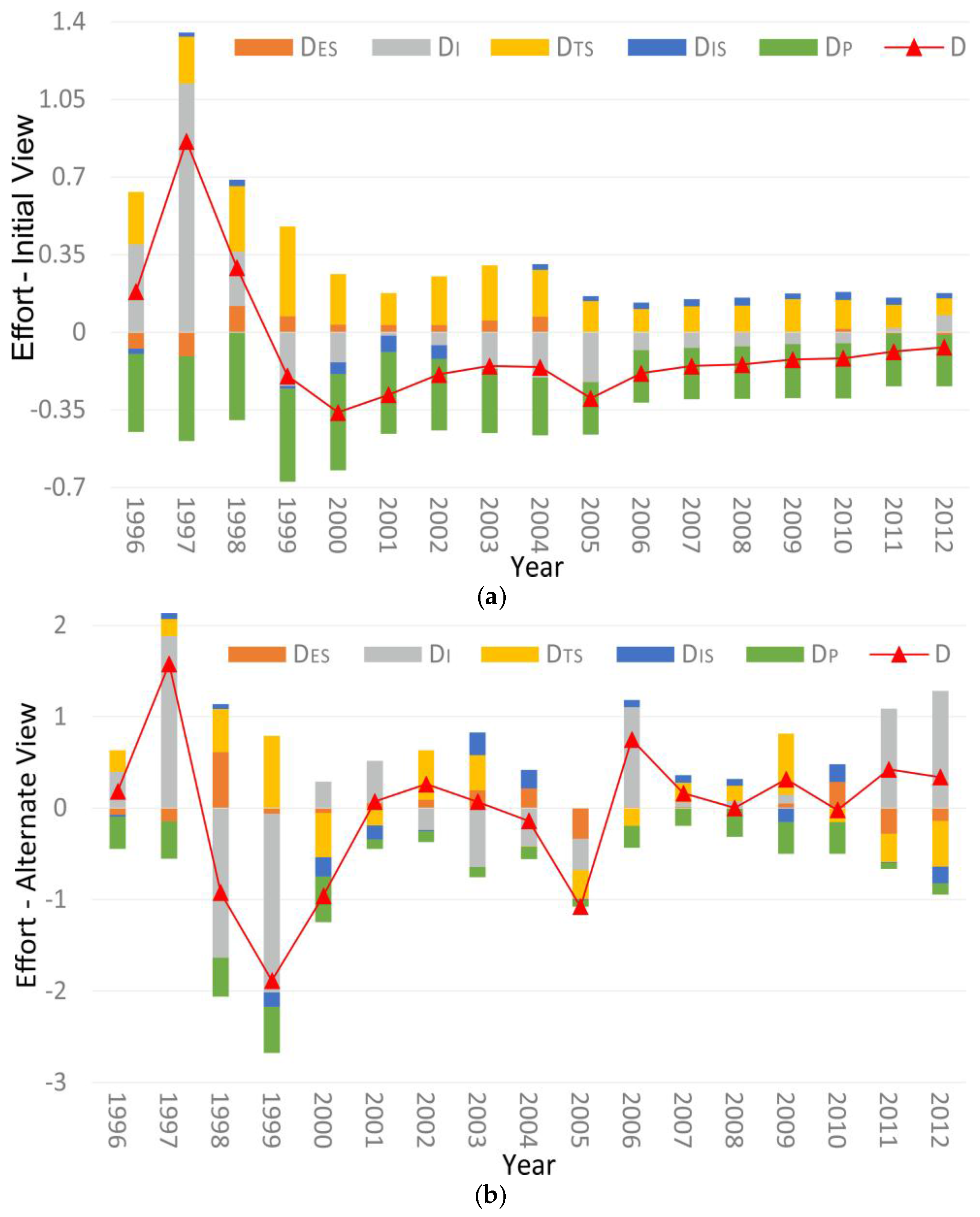
• D ≥ 1 denoting strong decoupling effort;
• 0 < D < 1 denoting weak decoupling effort;
• D ≤ 0 denoting no decoupling effort.

3. Results

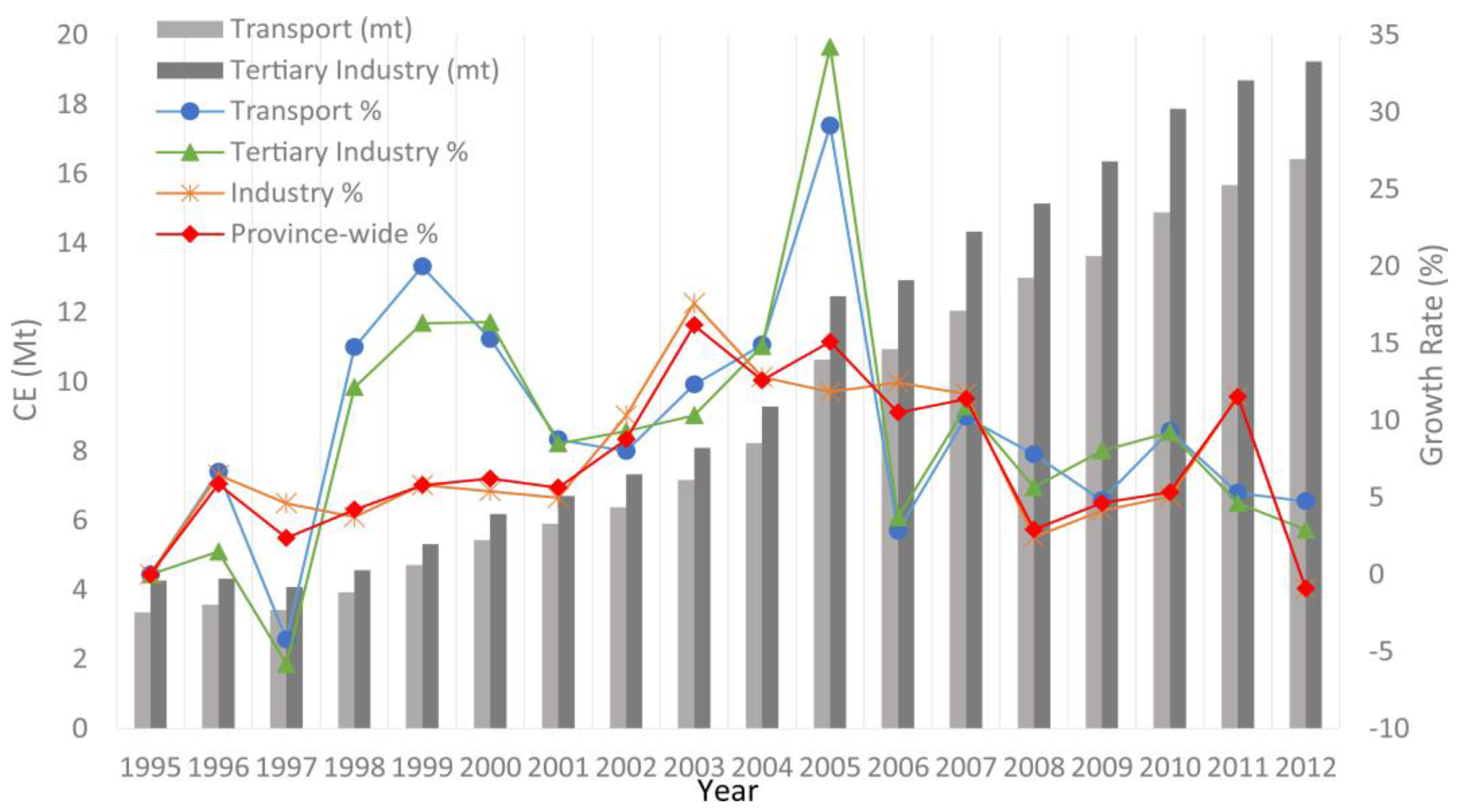
3.1. Analysis on Carbon Emissions

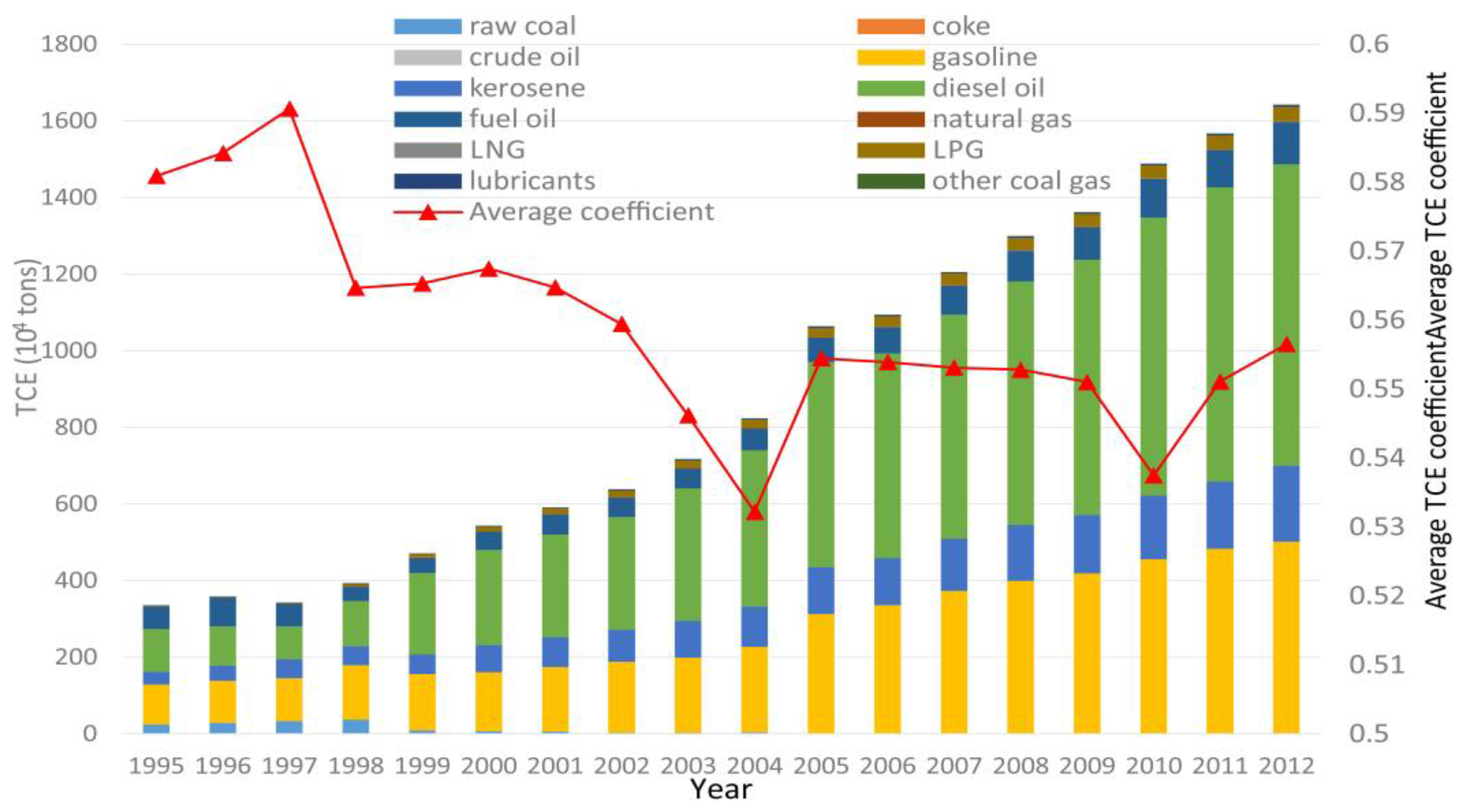
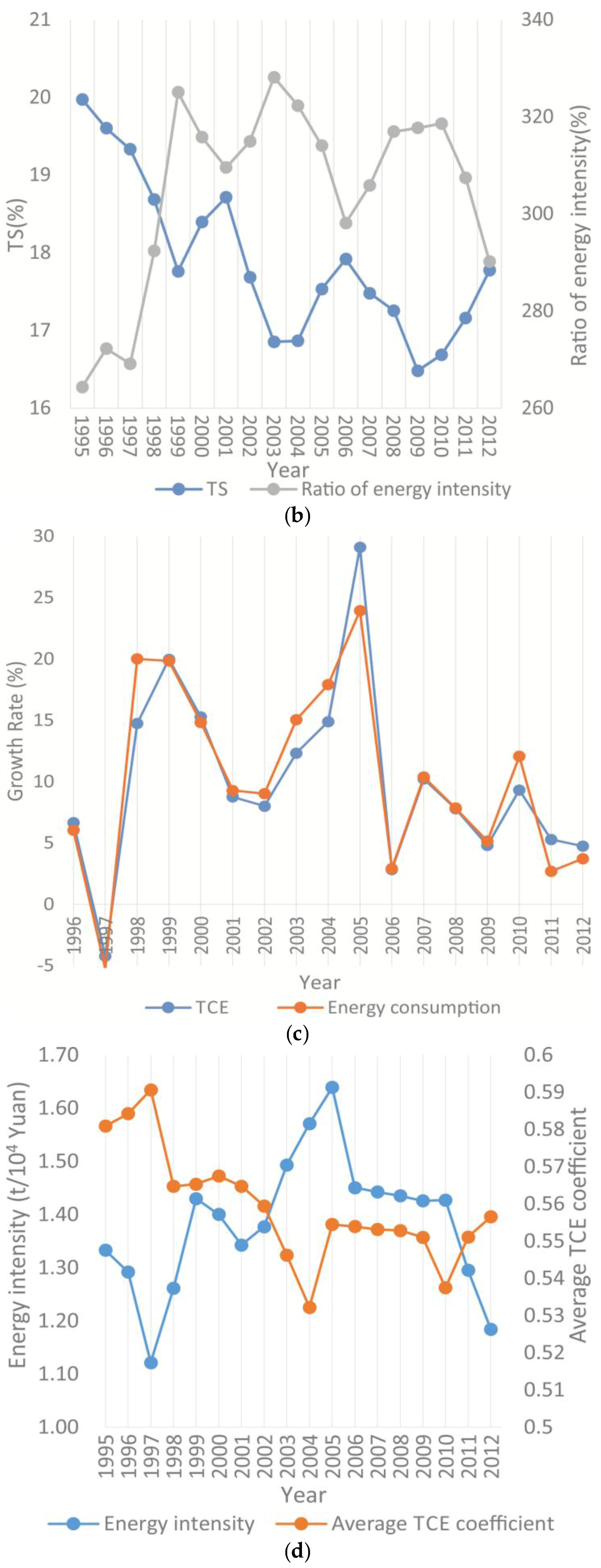
3.1.1. Macro-Level: Energy-Related Carbon Emissions of Transport

The estimated results (Figure 1) showed that the energy-related TCE in Guangdong rose from 3.35 million tons in 1995 to 16.42 million tons in 2012, an increase of nearly five-fold in 18 years. With the exception of a temporary recession in 1997 due to the Asian financial crises, Guangdong’s TCE kept increasing. The annual growth rate was fluctuating from −4.22% to 29.12% and then kept below 10.22% since 2006. The average annual growth rate of CE in transport, tertiary industry, secondary industry and province-wide total were 10.03%, 9.57%, 7.64% and 7.53% respectively. The growth rate of CE in transport was even higher than that of both total CE and each main industry within Guangdong. TCE accounted for 86% of the tertiary industry CE on average, and its remarkably consistent annual increase rate stabilized tertiary industry CE at a relatively high level. Therefore, if improving the proportion of the tertiary industry in GDP is a good way to reduce TCE, optimization of energy efficiency and structure in the transport sector must happen simultaneously.

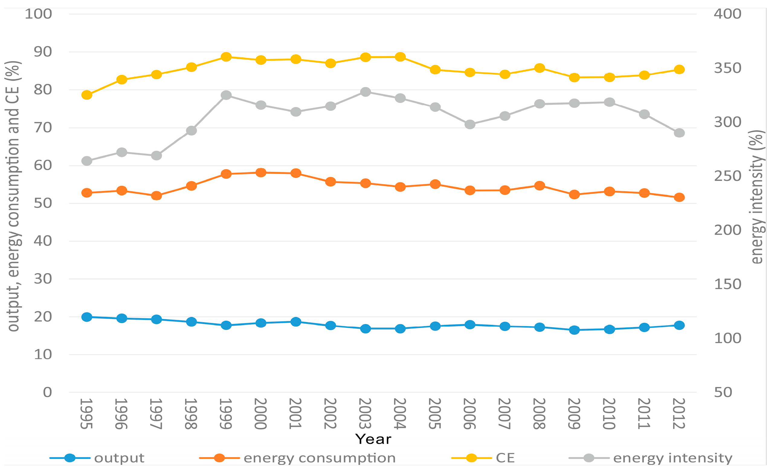
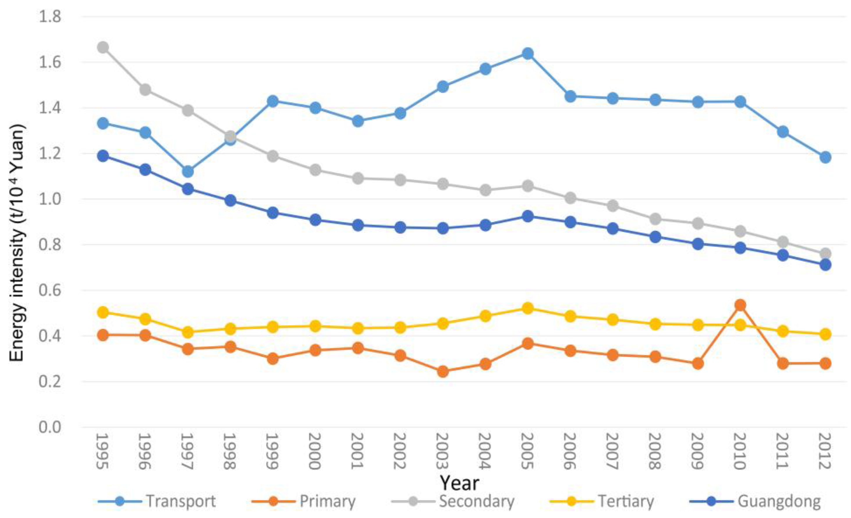
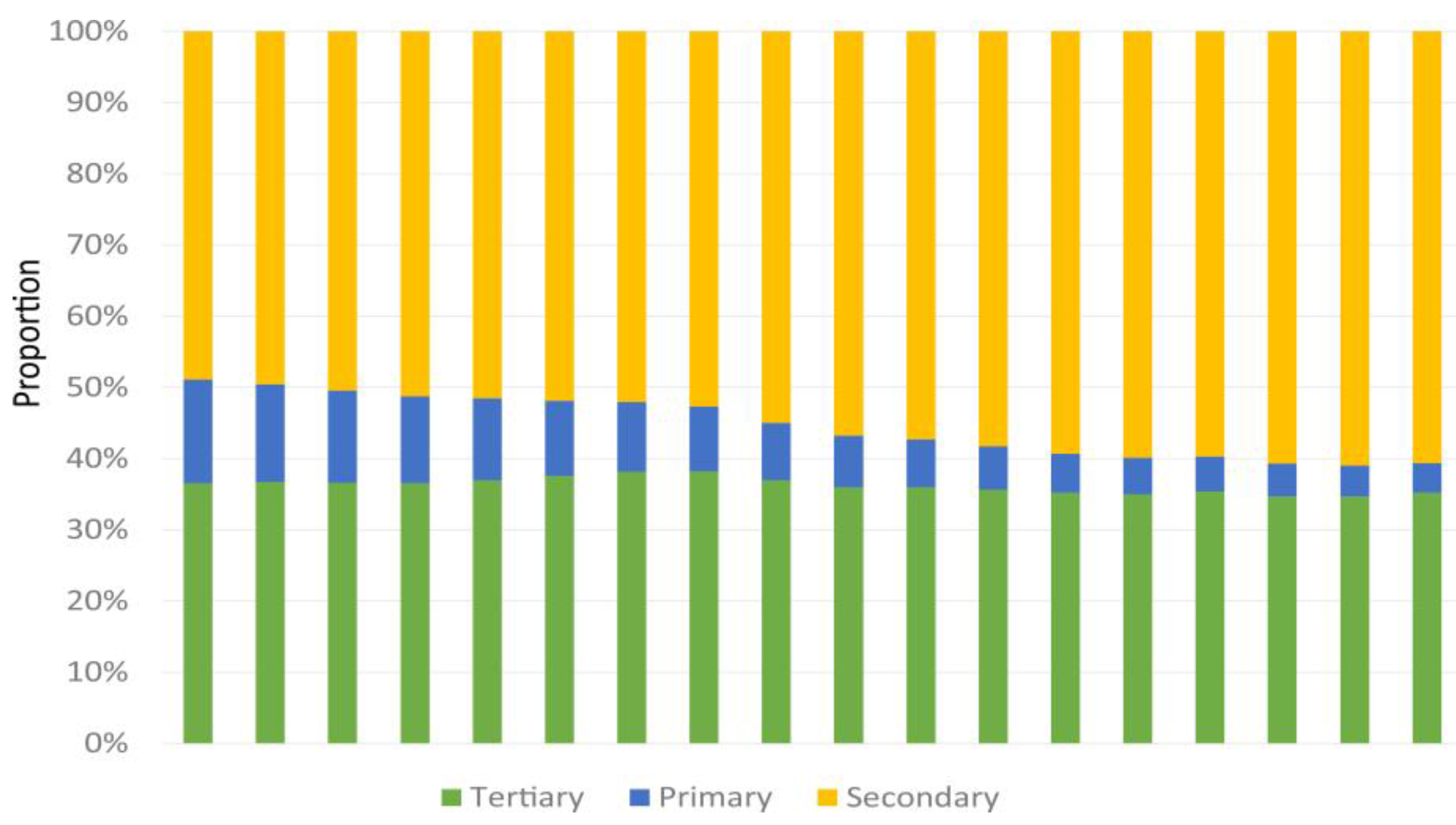
3.1.2. Micro-Level: Energy Intensity and Structure

Generally speaking, the improvement of energy efficiency is the primary driving force behind TCE reduction. With the development and renovation of technology, energy intensity of the secondary industry were continually descending (see Figure 2), which directly led to declining intensity of all industries’ total energy consumption. Intensity of primary and tertiary industries were kept below 0.6 and showed a bit of decrease after 2005. Transport, on the other side, has an energy intensity higher than that of all other sectors. Energy intensity of transport was continuing rising from 1995 to 2005, stayed steady for five years in 2005–2011, and fell sharply in 2011–2012. This indicated that related policies and techniques worked after 2005, and played better after 2010.

Over the period of 1995–2012, fossil energies, especially diesel contributed the most to TCE. Among the fossil energies, TCE from raw coal, coke and crude oil were at a low level and showed a significant reduction since 1998. This was mainly due to the gradual replacement of coal-based and energy-intense locomotives by electric or diesel ones. With the rapid development of railway electrification, the demand of coal was greatly reducing, and so was the coal-related CE.

The increment of CE from fuel oil and kerosene were on an intermediate level. Fuel-oil-related CE fluctuated but showed a generally rising trend during the studied period. With the development of the water transport, large vessels, deep water and specialized wharfs were be widely used. The combined effect of increasing waterborne demands and optimizing energy efficiency of waterborne equipment made the fuel-oil-related CE fluctuating. In the coming years, the Belt and Road Initiative will help in prospering the water transportation, as Guangdong was one of the main starting points of the Marine Silk Road. Therefor the growth of the fuel-oil-related CE may accelerate.

On the other hand, due to the rapidly increasing scale of kerosene-based air transport, steadily continuing growth was scored in kerosene-related CE. Its annual average growth rate was 11.39% between 1995 and 2012, which was even 1% higher than gasoline-related CE, although gasoline-related CE reached a level 2.5 times higher than kerosene in 2012. In the foreseeable future, with the development of international civil aviation and international tourism, kerosene consumption and related carbon emissions will keep growing rapidly.

Gasoline and diesel contributed the most to TCE. Figure 3 shows that the proportion of gasoline-related TCE was kept near one third of the total steadily. However, the proportion of diesel-related TCE increased from one third to half within the studied years. This is caused by increased diesel consumption due to the usage of trucks for road transport, which was, is and will remain the primary mode of transport in Guangdong. But it should be noticed that there was a reduction of growth rate since 2007.

As for clean energy, it had a rapid growth but still accounts for a very small slice among all energy types. Guangdong's government had taken actions to promote clean energy by a series of policies since 2005. In the Pearl River Delta, almost all taxis and buses were using liquid petroleum gas (LPG) since 2011, and are going to be upgraded to liquid natural gas (LNG) for its higher efficiency and eco-friendliness. This is potentially a great way to support TCE reduction in Guangdong.

Therefore, from a micro-perspective, petroleum products took a dominant role in transport sector within Guangdong’s CE structure during the studied years. This was not good for TCE reduction. However, clean energies have many unique advantages and will in no doubt be of growing importance in future.

3.2. Analysis on Decoupling Indexes

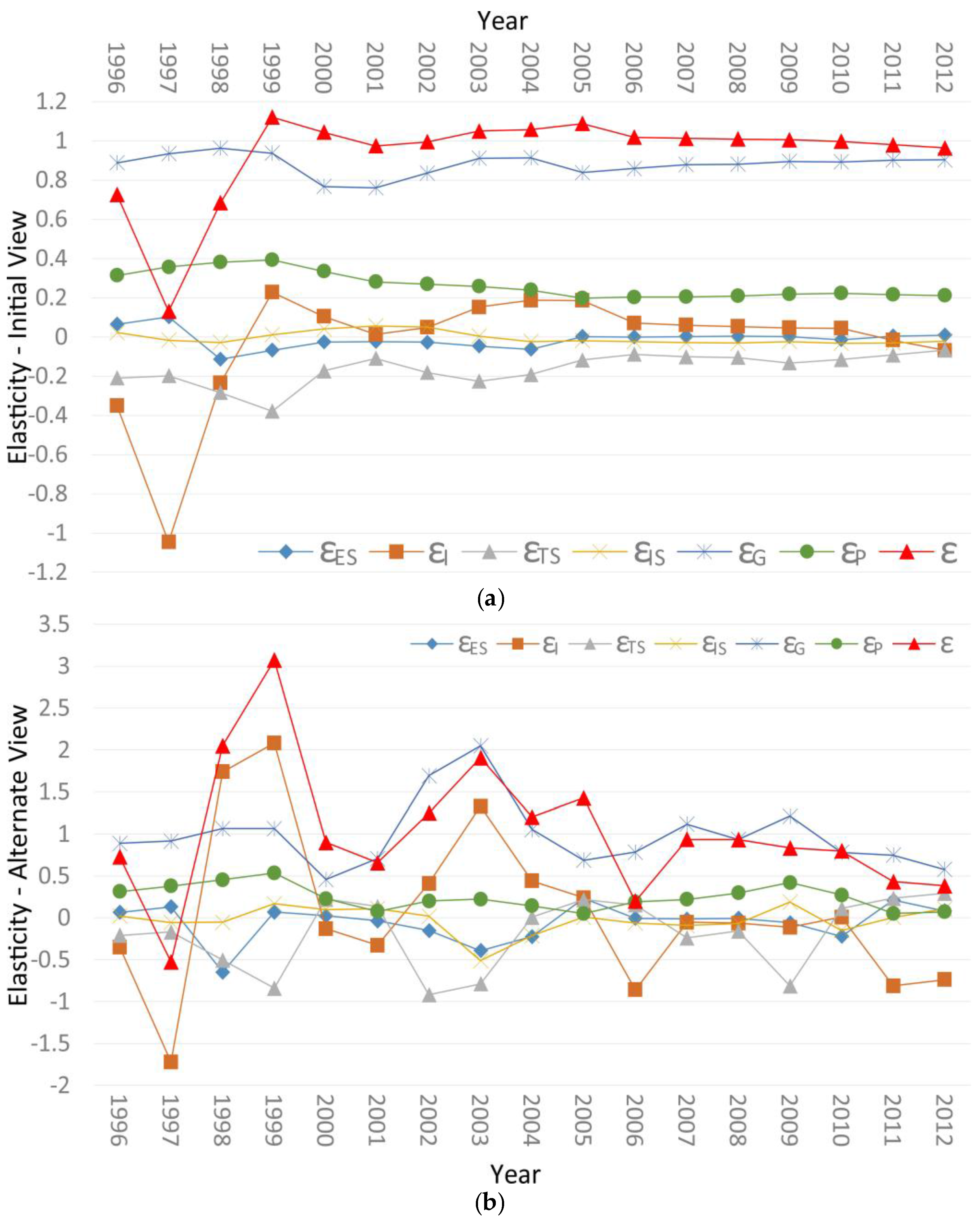
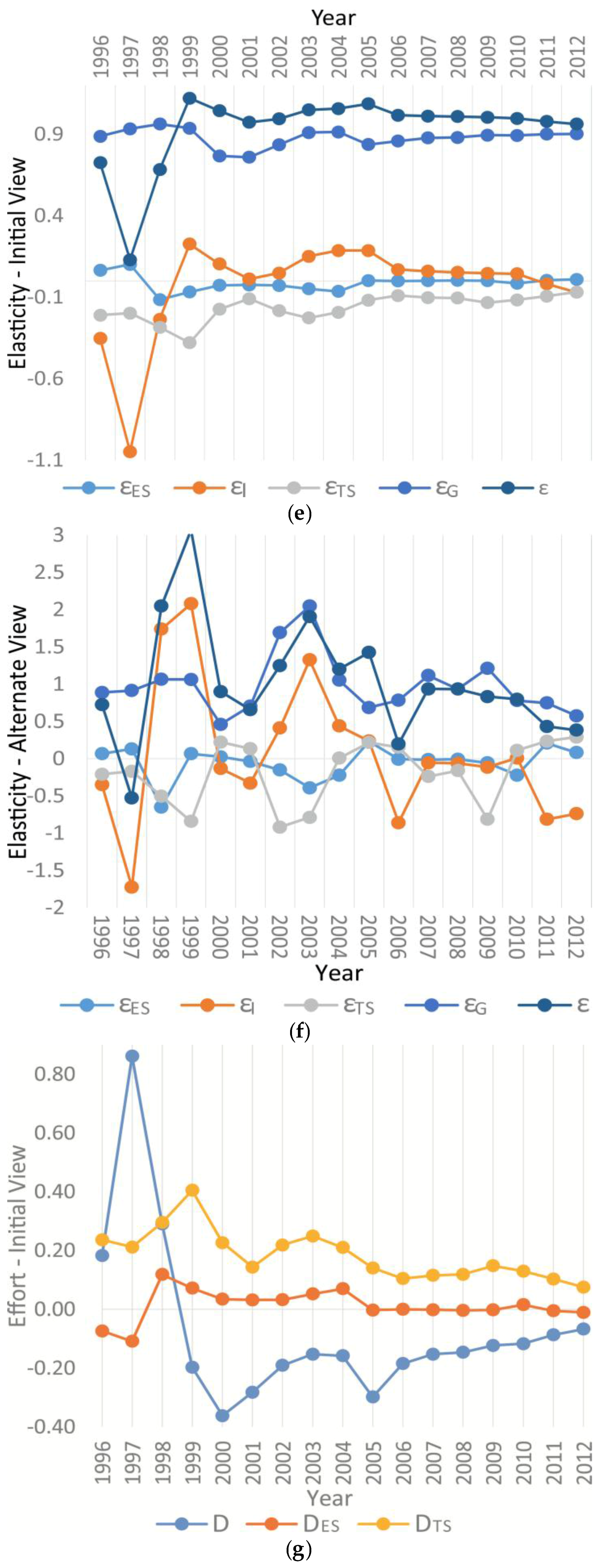
3.2.1. Decoupling Elasticity

Decoupling elasticity values and states of the transport sector in Guangdong can be seen in

Table 1. The elasticity values and states of CE in multiple time scales and output of transport sector in Guangdong.

Time Series	Initial						Alternate
	0	t	ΔCE	ΔTO	ε	State	0	t	ΔCE	ΔTO	ε	State
1 year	1995	1996	22.33	40.78	0.73	WD	1995	1996	22.33	40.78	0.73	WD
	1995	1997	7.21	84.08	0.13	SD	1996	1997	-15.11	43.29	-0.53	SD
	1995	1998	57.70	118.70	0.68	WD	1997	1998	50.49	34.62	2.05	END
	1995	1999	136.22	150.34	1.12	EC	1998	1999	78.52	31.64	3.07	END
	1995	2000	208.24	251.02	1.04	EC	1999	2000	72.02	100.68	0.90	EC
	1995	2001	255.81	346.48	0.97	EC	2000	2001	47.57	95.46	0.66	WD
	1995	2002	303.11	395.61	0.99	EC	2001	2002	47.30	49.13	1.25	END
	1995	2003	381.79	446.21	1.05	EC	2002	2003	78.68	50.60	1.91	END
	1995	2004	488.63	552.53	1.06	EC	2003	2004	106.85	106.32	1.20	END
	1995	2005	728.57	737.63	1.09	EC	2004	2005	239.93	185.10	1.43	END
	1995	2006	758.62	928.46	1.02	EC	2005	2006	30.05	190.83	0.20	WD
	1995	2007	870.37	1078.23	1.01	EC	2006	2007	111.76	149.77	0.94	EC
	1995	2008	964.36	1205.18	1.01	EC	2007	2008	93.99	126.95	0.93	EC
	1995	2009	1026.85	1300.76	1.00	EC	2008	2009	62.50	95.58	0.83	EC
	1995	2010	1153.78	1508.19	1.00	EC	2009	2010	126.93	207.43	0.80	WD
	1995	2011	1232.51	1763.50	0.98	EC	2010	2011	78.72	255.31	0.43	WD
	1995	2012	1306.94	2059.24	0.96	EC	2011	2012	74.43	295.74	0.38	WD
6 years	1995	2000	208.24	251.02	1.04	EC	1995	2000	208.24	251.02	1.04	EC
	1995	2006	758.62	928.46	1.02	EC	2001	2006	502.81	581.98	1.08	EC
	1995	2012	1306.94	2059.24	0.96	EC	2007	2012	436.56	981.01	0.68	WD
5-year plan	1995	2000	208.24	251.02	1.04	EC	1995	2000	208.24	251.02	1.04	EC
	1995	2005	728.57	737.63	1.09	EC	2000	2005	520.32	486.60	1.18	EC
	1995	2010	1153.78	1508.19	1.00	EC	2005	2010	425.22	770.56	0.72	WD
	1995	2012	1306.94	2059.24	0.96	EC	2010	2012	153.15	551.05	0.42	WD

The name of state: “WD” = Weak decoupling; “SD” = Strong decoupling; “EC” = Expansive coupling; “END” = Expansive negative decoupling. Which could also be seen in the Abbreviations.

. In the first three years, the elasticity state of accumulated decoupling changed from WD (weak decoupling) to SD (strong decoupling) and back to WD. The outlier appeared in 1997 was due to the Asian Financial Crisis, in which TCE did decrease while transport output was still slowly growing in Guangdong. Ever since 1999, it remained at a state of EC, in which the elasticity value was within a relatively narrow band from 0.96 to 1.12. There was a weak declining trend after 2005, where elasticity value dropped from 1.09 to 0.96. From a yearly perspective, the elasticity values demonstrated much more volatile fluctuations, ranging from −0.53 to 3.07 before entering a relatively steady decline from 1.91 in 2003 to 0.38 in 2012, corresponding to a decoupling state change from SD to expansive negative decoupling (END) and eventually to WD. With the exception of the outlier in 1997, the smallest yearly decoupling value showed in 2006, in which the yearly decoupling state turned from END to WD, with no END state seen afterwards. It highlights that transport growth was accompanied by a substantial increase in environmental pressure, though a significant improvement was seen after 2006. The decoupling state in two different perspectives from 2010 to 2012 varies, indicating relatively alleviated environmental pressure compared to preceding years, (a state of WD in alternate years) which is still remarkable (a state of EC in initial years) compared to1995.

The different trends in initial and alternate perspectives could be seen with a time scale of 6 years. If we set the time interval as 6 years, the studied period could be divided into three portions. When compared to 1995 (initial view) the decoupling elasticity remained in the state of EC, while the values went down from 1.04 to 0.96, and declined a little faster in the later period. In the alternate view, the elasticity values grew from 1.04 to 1.08 at first and then dropped sharply to 0.68, and the elastic state advanced from EC to WD.

Similar trends can be demonstrated if we set the time interval as five years, which corresponds to China’s five-year development plans. The end points in both views were the finish years of the plans, and the start point in initial view was 1995 and in alternate perspective was the last finish year of the plans. In this time scale, the elasticity values rose a bit in the former two plans, and then fell in the latter two plans. The decrease was much sharper in the alternate views and the elastic state turned from EC to WD in the 11th Five-Year Plan (2006–2010).

Overall, the initial decoupling state of transport in Guangdong was EC, and the alternate view displayed an improvement from EC to WD. In both views elasticity state improvement after 2005 can be seen by all three time scales, though they showed the quite different trends. By associating them, we could tell more details of the decoupling path in Guangdong. In this case, an investigation in multiple views of time seems quite necessary.

3.2.2. Decomposition Analysis

The decoupling analysis could reflect the environmental burden that transport formed, and by the decomposition method we could identify the driven forces behind the increasing CE [23,24,33,47,48]. Combining them together gives a more complete picture of Guangdong’s decoupling path. Contribution of six factors to elasticity are seen in Figure 4 and

Table 2. The proportion of decomposition factors of the elasticity value.

Year	Initial							Alternate
	εES	εI	εTS	εIS	εG	εP	ε	εES	εI	εTS	εIS	εG	εP	ε
	%	%	%	%	%	%	%	%	%	%	%	%	%	%
1996	8.98	−48.45	−28.97	2.95	122.40	43.09	100	8.98	−48.45	−28.97	2.95	122.40	43.09	100
1997	78.24	−808.70	−152.86	−13.13	721.21	275.25	100	−25.00	327.04	32.27	10.88	−173.57	−71.64	100
1998	−16.74	−34.42	−41.63	−4.07	141.04	55.82	100	−31.72	84.93	−24.59	−2.69	51.95	22.13	100
1999	−6.01	20.20	−33.82	1.01	83.54	35.08	100	2.17	67.70	−27.40	5.43	34.63	17.48	100
2000	−2.53	9.97	−16.66	3.85	73.43	31.94	100	2.78	−14.69	24.69	10.90	51.03	25.29	100
2001	−2.50	1.26	−11.23	5.65	78.00	28.82	100	−5.74	−49.95	20.39	16.41	107.52	11.38	100
2002	−2.75	4.92	−18.37	5.11	83.99	27.10	100	−12.22	32.85	−73.60	1.47	135.39	16.11	100
2003	−4.55	14.45	−21.62	0.36	86.77	24.60	100	−20.58	69.60	−41.35	−26.74	107.38	11.69	100
2004	−6.04	17.65	−18.19	−2.33	86.37	22.54	100	−18.67	36.49	0.54	−17.67	87.51	11.79	100
2005	0.20	17.13	−10.83	−1.72	77.04	18.19	100	16.12	16.61	15.20	0.41	48.12	3.54	100
2006	0.00	6.87	−8.83	−2.39	84.40	19.95	100	−3.54	−438.52	78.01	−31.41	399.91	95.55	100
2007	0.13	5.93	−10.03	−2.93	86.75	20.16	100	−1.49	−5.80	−25.61	−9.89	119.33	23.47	100
2008	0.30	5.24	−10.39	−3.16	87.27	20.73	100	−0.71	−6.74	−17.10	−7.26	100.06	31.75	100
2009	0.18	4.62	−13.20	−2.33	89.05	21.67	100	−6.94	−13.79	−97.87	22.42	145.77	50.41	100
2010	−1.41	4.42	−11.63	−3.28	89.54	22.37	100	−27.89	1.05	14.00	−18.86	97.76	33.93	100
2011	0.44	−1.79	−9.48	−3.14	92.00	21.98	100	48.48	−188.31	54.12	0.94	172.90	11.87	100
2012	0.96	−7.19	−7.09	−2.28	93.71	21.88	100	21.21	−193.52	75.80	27.49	150.83	18.19	100
ME97 1	−1.96	1.30	−17.00	−0.54	90.96	27.24	100	−1.86	−40.66	−3.36	−1.63	120.78	26.73	100

¹ “ME97” means the mean values of each factors excluding the year of 1997.

. Due to the outlier in 1997, this paper estimated the average values of each factors excluding the year of 1997, named “ME97” in the table.

In the initial views, over the studied years, TS was the only effect that always played an inhibiting role in the increase of TCE, which accounted for average of –17.00%. Though TS’s absolute contribution to TCE reduction was rising from 0.06 million to 0.93 million tons, it was still dwarfed by the effect of G and P. G and P factors had the largest negative effects on elasticity, which on average occupied 90.96% and 27.24% of the overall elasticity respectively. The ES, I and IS factors had alternations of positive and negative effects and accounted for average −1.96%, 1.30% and −0.54% respectively. Among them, I factor experienced the most volatile changes, but saw further optimization since 2004. ES and IS factors had the smallest proportions and variations. In 2012, the ES, G and P effects were positive; I, TS and IS effects were negative. The initial effects of G and P factors had the largest impact which accounted for 93.71% and 21.88%. The proportion of ES, I, TS and IS factors were much lower at 0.96%, −7.19%, −7.09% and −2.28%, respectively.

Much larger variations can be seen in the decomposition results from an alternate years’ perspective. G and P effects remained stably positive and contributed the most from 1995 to 2012, accounting for on average 120.78% and 26.73% of the elasticity value respectively. The G effect was definitely in the majority. There was large fluctuation of I effect, whose contribution to TCE fluctuated from −1.48 million to 0.55 million tons, and the average proportion was −40.66%, while ES, TS and IS effects waved much tenderly and occupied −1.86%, −3.36% and −1.63%, respectively. Although there were four factors had inhibited function according to ME97, only I factor maintained negative in 2012.

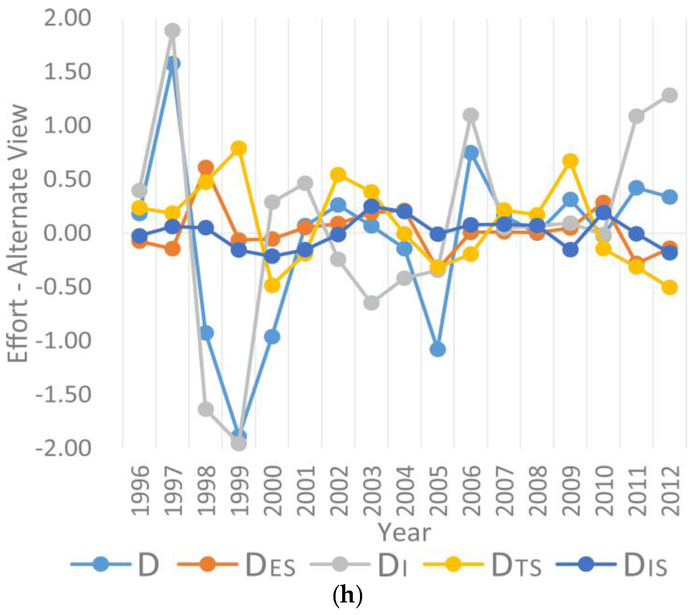
3.2.3. Decoupling Effort

The effort could effectively figure out the degree of each factor to which they made to reduce TCE by dissociating transport output from TCE (Figure 5). The initial effort dramatically peaked from 0.18 to 0.86 in 1997 and then dropped rapidly to 0.29 in the next year. After that, it fluctuated at a quite low level of −0.36 to −0.15, suggesting it denoted no decoupling effort since 1999. However, there was a smoothly growth trend from 2005, and the effort value rose from −0.30 to −0.07. If this trend keeps up, the value will be positive soon. Among the components, I effort always had a similar trend with the total effort, except it became positive since 2011, which took the lead of the total effort. Though the value of TS effort waved from 0.08 to 0.40, it still had the biggest and positive effort (other indices were relatively lower or negative). On the contrary, P effort was the lowest and always negative, which waved from −0.44 to −0.23, and showed a slightly growth trend since 1999 because of the decline of the growth rate of population. Additional, the value of ES and IS both hovered near zero, which showed their inconspicuous roles in the TCE reduction.

When set the previous year as the base year, we got the alternate efforts. The total alternate effort showed high volatility over the research period, which waved widely from 1.58 to −1.89 and then down to −1.08 in 2005. Afterwards, it mostly remained positive and fluctuated more smoothly from −0.02 to 0.75. It indicated that the alternate effort was volatile but had obvious improvement in reducing TCE. I factor presented a similar trend with total efforts as well, while changed more acutely which waved from −1.96 to1.88. In 2011 and 2012, I effort was 1.09 and 1.28 which showed its effort was enhancing and strong. The value of TS factor did not show the consistent direction which changed widely from −0.48 to 0.79. P effort was always negative but the value was bigger than it in initial years, which changed from −0.50 to −0.07. The values of ES and IS were very small and negative off and on within the research years.

In addition, no matter in the perspective of initial or alternate years, the effort of energy intensity and total effort always showed the same variation during the research years, indicated that reducing energy intensity may be one of the most important approach to enhance the decoupling effort.

4. Discussion

4.1. Overview of the Decoupling

In this paper, we applied a decomposition technique to analyze TCE and its components in Guangdong Province, and measured the environmental pressure from transport growth by bonding the LMDI method with decoupling elasticity over the period 1995–2012. 2005 was a turning point, when energy-saving and emission-reduction were emphasized and the optimization of industrial structure came into play in China, especially in developed areas like Guangdong Province. The results showed that energy-related TCE in Guangdong had a continuous growth within the studied period, which was consistent with researches suggesting that TCE in Guangdong kept improving [6,7].

The elasticity of transport in Guangdong was mainly in a state of EC, which indicated that transport growth was accompanied by a substantial pressure on the environment. Additionally, there was a slightly declining trend of the elasticity value since 2005, which showed that new environmental friendly policies worked to some extent. Besides, the reduction effort to TCE were positive within the first three years, but turned negative in a sudden and then remained negative till 2012. There was also a slightly increasing trend of effort after 2005, which correlates well with the overall pattern shown by the decoupling elasticity. The optimization of tertiary industry structure was the main inhibiting factor of TCE increase. However the rapid economy and population growth were powerful at boosting TCE, resulting in elasticity rising directly. Energy structure and industrial structure played a very weak role in TCE reduction, which should be focused on in the future.

GDPPC and Population were the most powerful boosters of TCE. Accompanied by the faster process of industrialization and urbanization and the large amount of population, citizen mobility as well as transportation distance and volume are to spurt. In the meantime, the rapid growth in economic output could meet the surging demand of national development and higher life quality expectations. Correspondingly, energy consumption per capita and TCE will be ascending, leading to increased pressure of TCE reduction in Guangdong.

Evaluation of effort provides important insights into the development of transport in Guangdong that goes beyond decoupling elasticity analysis. After removing the G effect, the effort remained negative, which indicated that it is a tough task to reach the level of effort required for strong decoupling. Therefore energy structure, industrial structure and energy efficiency should all be emphasized in realizing the harmonious development of economy and environment. Energy consumption structure is a key factor to TCE, while it played an unimportant role in inhibiting the elasticity in Guangdong. On the other hand, energy intensity contributions to elasticity and its effort were extreme volatile, suggested that the TCE reduction effect of energy intensity was not stable enough and there is a long march. The government should promote clean energy and public transport to enhance the progresses of energy efficiency of the transport sector.

As the most developed province of China, Guangdong has both strong development of traditional industries as well as superior conditions for emerging industries. Nevertheless, the secondary industry is still the dominant (Figure 6), accounted for about 60.6% of the whole economic output in Guangdong in 2012. Tertiary industry, on the other hand, kept close to its average portion of 36.04% steadily, thus the contribution of industrial structure’s effect to elasticity and its effort was inconspicuous. In fact, many industrial policies have been promoted to adjust the industrial structure both on provincial and the national levels since 2005, which suggests that optimizing industrial structure is a long-term process. Therefore, we should continue to focus on it and accumulate practical experience.

4.2. Tertiary Industrial Structure

According to the decomposition and decoupling analysis, it was the only steady and inhibitive factor of elasticity and played a significant positive role in decoupling effort. Figure 7 illustrated an ironic structure of tertiary structure where the transport sector produced less than 1/5 of the total tertiary industry economic output, but consumed more than half of the fuel (standard coal), and emitted more than 4/5 of the carbon. The energy intensity of transport was more than three times higher than tertiary industry average. Therefore, if improving the proportion of the tertiary industry in GDP is a good way to reduce TCE, optimizing energy efficiency and energy structure of transport must be the key points. The government should motivate the energy efficiency improvement of transport to make the tertiary industry be real low-carbon industry. On the other hand, the other 82% output which only emitted about 14% carbon must be produced by real clean service sectors of the tertiary industry. These sectors are the real ones to be promoted.

4.3. Time Issues of the Model: Baseline and Time Scale

By considering more time issues, this paper has tried to dig the greatest potential interpret-ability of the models. Firstly, we picked an 18-year research time which is long enough to cover the turning point, in which China started to apply scientific outlook on development. And we do prove that 2005 is a most meaningful year, after which most of indices were optimized (except population). It indicated that policies had a decisive role in the field of environmental conservation.

Secondly, when analyzing the decoupling elasticity we used three time scales. Comparing adjacent years, which utilizes a time scale of one year, gives most detailed information. Five-year periods reveal an important correlation between National Five-Year Plans and decoupling effort. A scale of six years divides the studied time into three equal parts. The switch towards WD in 2010 is seen with one-year and five-year views while six-year makes it less visible. Choosing a proper time scale requires thinking twice, and oversimplification can lead to loss of important information.

In addition, we consistently analyzed elasticity and its effort in both initial and alternate views by using two different years as baselines. The development of elasticity was smooth in initial years view while more volatile fluctuations can be seen from an alternate years’ perspective. As a consequence, we could disclose more information with an alternate years view. On the one hand, both the elasticity state and decoupling effort achieved overall improvement during the studied period, but there were too many intensive fluctuations. For example, from 2005–2012, the effect of energy intensity improved in initial perspective (effect on both of elasticity state and decoupling effort), while it experienced improvement, rebound, period-slump, and improvement again in alternate view, which presented a periodic pattern, and so did other indices. This suggests the lack of inner drives of CE reduction. If the inner drives such like energy efficiency and industrial structure had steady and enormous progress, the elasticity state and its effort should be promoted continuously. Thus, there must be other stronger factors guiding the decoupling state, for example policy, as discussed below.

4.4. Five-Year Periodic Pattern

4.4.1. Periodic Variation of Each Plan

The studied period spans across three and a half Five-Year Plans. With the exception in 1997 which was affected by an economic crisis, the decoupling analysis showed a five-year periodic variation pattern, as seen in Figure 8 and

Table 3. The periodic variation of the factors’ value in each plan.

Factor	Indicators	Variation Pattern of 5-Year Plans
Economy	GDP growth	Always high, much higher in the final year of every plan
	GDPPC growth
	TO growth	“∪”-shape, with minimum values in the middle of each plan
	TS
Environment	Energy consumption	Minimum values at the beginning of each plan, rising towards a high level near the end
	TCE growth
	Average TCE coefficient	Generally showing“∪”-shapes, trough of 11th 5-Year Plan delayed
Comprehensiveness	Decoupling index	“∩"-shape, with maximum values in the middle of each plan
	Decoupling effort
	Energy intensity of transport to tertiary industry
	Energy intensity	Peaks around 1995, 1999, 2005 and 2010, close to the ending of each plan

.

The best state of effort, energy intensity, energy consumption, average TCE coefficient and tertiary structure were in the middle years of every plan, while TO growth and energy intensity were at their worst during the same time.

It is conceivable that Five-Year Plans had a huge impact on economic and TCE-related indicators. At the last year of each five-year period, economic indicators like GDP growth and transport output in Guangdong both increase. However, they had different overall patterns. GDP growth always remained at a relatively high level, and its range of change was small. Transport output, on the other hand, only saw a dramatic growth in the ending years of two plans, while in the middle years of each plan it stays on a low level. Its fluctuation was quite drastic.

Environmental pressure indicators such as TCE growth, energy consumption growth and average TCE coefficient showed an inverse tendency. In the final year of each plan, these indicators showed a significant boost of environmental pressure, while the least stress appeared in the middle years within each plan.

Because of the five-year periodic variation pattern of economic and environmental indicators, comprehensive indicators such as decoupling elasticity and effort present periodic changes correspondingly. In the final year of each plan, the elasticity state turns better. However, the effort is worsened, while energy intensity increases. It indicated that in the final year of each plan, the influence of GDPPC was considerably higher than any other indexes, and all the comprehensive indicators demonstrated signs of increasing environmental pressure.

In addition, in the end year of each plan, the ratio of output growth between transport and tertiary industry, also known as tertiary industrial structure, increased, while the ratio of energy intensity between the two decreased. In fact, both transport and tertiary industry achieved a higher output growth in the end year of every plan. Because the transport output growth was more volatile, the value of TS was increasing, thus the tertiary industry structure deteriorated.

The five-year periodic variation pattern above implicated one of the problems in Guangdong, that we always prefer economic quantity over quality. In fact, Guangdong had successfully completed or exceeded the targets of every Five-Year Plan, so it is possible to reduce TCE while meeting economic expectations at the same time. Guangdong should try to unlock its huge potential to improve energy efficiency and reduce carbon emissions.

4.4.2. Variation of the Inter-Plans

During the period of three and a half Five-Year Plans, the intensity of fluctuation became more and more limited. Since 2007, there was a constant trend of improvement in decoupling elasticity and its effort, especially in the first two years of the 12th Five-Year Plan (2011–2012).

This was due to Chinese government has given more attention to environmental conservation and energy efficiency. During the 9th and 10th Five-Year Plan, China concerned more about economy growth and did make remarkable progress. But the nation increasingly came to realize that sole emphasis on GDP is not good for the sustainable development of the nation after seeing heavy environmental pressure and its consequence. In 2003, former Chinese chairman Hu put forward scientific development view. The 11th Plan (2006–2010) presented the serious problems related to the excessive consumption of energy and stated the reduction of energy consumption per unit of GDP as a main goal. Guangdong positively responds to the call and formulates the target to drop the energy consumption per unit GDP by 16% during the 11th Five-year plan compared to that in 2005. Specific environmental friendly measures were carried out with many outstanding achievements in TCE reduction, including elimination of low-tech productive capacity and replacement of high energy factories such as small thermal power stations and cement plants. Our government promised to reduce CO₂ emission per unit GDP by 40%–45% in 2020 compared to that in 2005 in Copenhagen Climate Change Conference in 2009. The “12th Five-Year Plan” (2011–2015) also focused on the reduction of energy intensity. Though only the first two years of the 12th Five-Year Plan fall into the studied time range, positive changes of elasticity and its effort is still significant. This period has been an important stage of the transformation in energy efficiency of China’s economy.

4.4.3. Summary

It’s said “Deadline is the first productivity”. This may apply to decoupling between TCE and economy. The National Five-Year Plans have made huge impact on economic and environmental development in Guangdong, which showed the five-year periodic pattern correspondingly. During the studied period, decoupling elasticity and its effort were at a very low level in the first two Five-Year Plans, the inner drives of TCE reduction were weak and passive. Things had changed after promoting the outlook of scientific development and taking actions to protect environment in the two later plans. The elasticity state and its effort were gradually optimizing. To achieve the state of strong decoupling, however, many long-lasting problems still need to be fixed. The latest progress happened at the Third Plenary Session of the 18th Central Committee in 2013, in which the government promoted the concept of ecological civilization, further enriching the theoretical system of the outlook of scientific development. All of these efforts will benefit the harmonious development of economy, society and environment in China.

There are major concerns of the impact of strict environmental conservation policy in many fields, especially in economic development. As such, environment protection needs strong support and promotion by the effective policies from the government.

5. Conclusions

In conclusion, the level of decoupling elasticity between transport output and TCE was relatively low over the studied years in Guangdong, especially when compared with the year of 1995, in which case it remained as EC. 2005 was a turning point, at which environmental protection was highly emphasized and the alternate elasticity started optimizing towards WD. By covering nearly a decade before and after the turning point, the effectiveness and significance of policy change was clearly shown. However, as seen from the data, the time frame used in the analysis can cause significant drift of decoupling and effort values, therefore it should be selected with caution. It’s also important to note that decoupling is relative, and in Guangdong’s case the selection of reference year can lead to fundamental change of the decoupling analysis’ result. With 1995 being the reference, we see a continuous trend of EC, while with 2005 there is a transition to WD.

Within all the factors taken into consideration, structure of tertiary industry displays highest level of impact on EC decoupling. Unfortunately, transport has a dominate role in tertiary industry. It’s accounted for the majority of output, energy consumption and intensity in tertiary industry. Thus we should pay more attention to the carbon emission reduction in transport sector by more targeted researches, policies and real actions.

Under high pressure from economy and population growth, decoupling and effort levels were mostly low within Guangdong throughout the studied years. Strong decoupling was actually achieved in 1997, as a result of the Asian economic crisis, accompanied by lowered employment rate and worsened quality of life, with little input from environmental protection policies. The high decoupling level was merely an economy-driven anomaly which dropped back to EC shortly after the crisis. The 2008 crisis, on the other hand, didn’t see significant change in decoupling level even though environmental protection policies are in place. At this time the decoupling effect was more controlled by non-economic inner-drivers, and remained stable. Suppressing the growth of economy and population is therefore not an effective method of achieving decoupling, while inner-drivers such as enhanced energy efficiency and optimized industrial structure demonstrate more consistent effect.

We also identified a strong pattern of periodic change in decoupling level controlled by the Five-Year Plan policy. The decoupling value tends to be low in the middle of each 5-year period and rise up near each 5-year mark. This effect highlights policy as one of the most important factor behind decoupling effort, dwarfing the impact from energy and industrial inner-drivers.

References

1. Talukdar, D.; Meisner, C.M. Does the private sector help or hurt the environment? Evidence from carbon dioxide pollution in developing countries. World Dev. 2001, 29, 827–840. [Google Scholar] [CrossRef]
2. Zhang, L.; Huang, Y.X.; Li, Y.M.; Cheng, X.L. An investigation on spatial changing pattern of CO2 emissions in china. Resour. Sci. 2010, 32, 211–217. [Google Scholar]
3. Yu, S.; Ma, C.; Wang, T.; Li, X. Preliminary comment on “Reduced carbon emission estimates from fossil fuel combustion and cement production in China“. Energy China 2015, 37, 27–31. (In Chinese) [Google Scholar]
4. Zhou, N.; Levine, M.D.; Price, L. Overview of current energy-efficiency policies in china. Energy Policy 2010, 38, 6439–6452. [Google Scholar] [CrossRef]
5. Zhou, G.; Chung, W.; Zhang, X. A study of carbon dioxide emissions performance of China’s transport sector. Energy 2013, 50, 302–314. [Google Scholar] [CrossRef]
6. Wang, W.; Kuang, Y.; Huang, N. Study on the decomposition of factors affecting energy-related carbon emissions in Guangdong Province, China. Energies 2011, 4, 2249–2272. [Google Scholar] [CrossRef]
7. Wang, W.; Kuang, Y.; Huang, N.; Zhao, D. Empirical research on decoupling relationship between energy-related carbon emission and economic growth in Guangdong Province based on extended kaya identity. Sci. World J. 2014, 2014, 782750. [Google Scholar] [CrossRef] [PubMed]
8. Kiang, N.; Schipper, L. Energy trends in the Japanese transportation sector. Transp. Policy 1996, 3, 21–35. [Google Scholar] [CrossRef]
9. Zachariadis, T. On the baseline evolution of automobile fuel economy in europe. Energy Policy 2006, 34, 1773–1785. [Google Scholar] [CrossRef]
10. Michaelis, L.; Davidson, O. GHG mitigation in the transport sector. Energy Policy 1996, 24, 969–984. [Google Scholar] [CrossRef]
11. Kwon, T.H. The determinants of the changes in car fuel efficiency in great britain (1978–2000). Energy Policy 2006, 34, 2405–2412. [Google Scholar] [CrossRef]
12. Stead, D. Transport intensity in Europe—Indicators and trends. Transp. Policy 2001, 8, 29–46. [Google Scholar] [CrossRef]
13. Preston, J. Integrating transport with socio–economic activity—A research agenda for the new millennium. J. Transp. Geogr. 2001, 9, 13–24. [Google Scholar] [CrossRef]
14. Tapio, P.; Banister, D.; Luukkanen, J.; Vehmas, J.; Willamo, R. Energy and transport in comparison: Immaterialisation dematerialisation and decarbonisation in the eu15 between 1970 and 2000. Energy Policy 2007, 35, 433–451. [Google Scholar] [CrossRef]
15. Chung, W.; Zhou, G.; Yeung, I.M.H. A study of energy efficiency of transport sector in China from 2003 to 2009. Appl. Energy 2013, 112, 1066–1077. [Google Scholar] [CrossRef]
16. Tirumalachetty, S.; Kockelman, K.M.; Nichols, B.G. Forecasting greenhouse gas emissions from urban regions: Microsimulation of land use and transport patterns in Austin, Texas. J. Transp. Geogr. 2013, 33, 220–229. [Google Scholar] [CrossRef]
17. Xu, B.; Lin, B. Carbon dioxide emissions reduction in China's transport sector: A dynamic var (vector autoregression) approach. Energy 2015, 83, 486–495. [Google Scholar] [CrossRef]
18. Papagiannaki, K.; Diakoulaki, D. Decomposition analysis of CO2 emissions from passenger cars: The cases of greece and Denmark. Energy Policy 2009, 37, 3259–3267. [Google Scholar] [CrossRef]
19. Baldwin, J.G.; Wing, I.S. The spatiotemporal evolution of us carbon dioxide emissions: Stylized facts and implications for climate policy. J. Reg. Sci. 2013, 53, 672–689. [Google Scholar]
20. Kang, Y.Q.; Zhao, T.; Wu, P. Impacts of energy-related CO2 emissions in China: A spatial panel data technique. Nat. Hazards 2016, 81, 405–421. [Google Scholar] [CrossRef]
21. Yuan, L.; Pan, J. Disaggregation of carbon emission drivers in kaya identity and its limitations with regard to policy implications. Adv. Clim. Chang. Res. 2013, 9, 210–215. [Google Scholar]
22. Andreoni, V.; Galmarini, S. Decoupling economic growth from carbon dioxide emissions: A decomposition analysis of Italian energy consumption. Energy 2012, 44, 682–691. [Google Scholar] [CrossRef]
23. De Freitas, L.C.; Kaneko, S. Decomposing the decoupling of CO2 emissions and economic growth in Brazil. Ecol. Econ. 2011, 70, 1459–1469. [Google Scholar] [CrossRef]
24. Diakoulaki, D.; Mandaraka, M. Decomposition analysis for assessing the progress in decoupling industrial growth from CO2 emissions in the eu manufacturing sector. Energy Econ. 2007, 29, 636–664. [Google Scholar] [CrossRef]
25. Hatzigeorgiou, E.; Polatidis, H.; Haralambopoulos, D. CO2 emissions, gdp and energy intensity: A multivariate cointegration and causality analysis for Greece, 1977–2007. Appl. Energy 2011, 88, 1377–1385. [Google Scholar] [CrossRef]
26. Kang, J.D.; Zhao, T.; Ren, X.S.; Lin, T. Using decomposition analysis to evaluate the performance of China’s 30 provinces in CO2 emission reductions over 2005–2009. Nat. Hazards 2012, 64, 999–1013. [Google Scholar] [CrossRef]
27. Liang, S.; Liu, Z.; Crawford-Brown, D.; Wang, Y.; Xu, M. Decoupling analysis and socioeconomic drivers of environmental pressure in china. Environ. Sci. Technol. 2014, 48, 1103–1113. [Google Scholar] [CrossRef] [PubMed]
28. Tapio, P. Towards a theory of decoupling: Degrees of decoupling in the eu and the case of road traffic in finland between 1970 and 2001. Transp. Policy 2005, 12, 137–151. [Google Scholar] [CrossRef]
29. Wang, W.; Liu, R.; Zhang, M.; Li, H. Decomposing the decoupling of energy-related CO2 emissions and economic growth in jiangsu province. Energy Sustain. Dev. 2013, 17, 62–71. [Google Scholar] [CrossRef]
30. Fouquet, R. Trends in income and price elasticities of transport demand (1850–2010). Energy Policy 2012, 50, 62–71. [Google Scholar] [CrossRef]
31. Lu, Q.; Yang, H.; Huang, X.; Chuai, X.; Wu, C. Multi-sectoral decomposition in decoupling industrial growth from carbon emissions in the developed jiangsu province, China. Energy 2015, 82, 414–425. [Google Scholar] [CrossRef]
32. Organization for Economic Cooperation and Development (OECD). Indicators to Measure Decoupling of Environmental Pressure from Economic Growth; Organization for Economic Cooperation: Paris, France, 2002. [Google Scholar]
33. Brizga, J.; Feng, K.; Hubacek, K. Drivers of CO2 emissions in the former soviet union: A country level IPAT analysis from 1990 to 2010. Energy 2013, 59, 743–753. [Google Scholar] [CrossRef]
34. York, R.; Rosa, E.A.; Dietz, T. Stirpat, ipat and impact: Analytic tools for unpacking the driving forces of environmental impacts. Ecol. Econ. 2003, 46, 351–365. [Google Scholar] [CrossRef]
35. Schipper, L.; Scholl, L.; Price, L. Energy use and carbon emissions from freight in 10 industrialized countries: An analysis of trends from 1973 to 1992. Transp. Res. D Transp. Environ. 1997, 2, 57–76. [Google Scholar] [CrossRef]
36. Greening, L.A.; Ting, M.; Davis, W.B. Decomposition of aggregate carbon intensity for freight: Trends from 10 OECD countries for the period 1971–1993. Energy Econ. 1999, 21, 331–361. [Google Scholar] [CrossRef]
37. Scholl, L.; Schipper, L.; Kiang, N. CO2 emissions from passenger transport—A comparison of international trends from 1973 to 1992. Energy Policy 1996, 24, 17–30. [Google Scholar] [CrossRef]
38. Schipper, L.; Steiner, R.; Duerr, P.; An, F.; Strom, S. Energy use in passenger transport in OECD countries—Changes since 1970. Transportation 1992, 19, 25–42. [Google Scholar] [CrossRef]
39. National Bureau of Statistics of China. National Economy Industry Classification Annotations 2011, 4th ed.China Statistics Press: Beijing, China, 2011.
40. Department of Energy Statistics, National Bureau of Statistics, China. China Energy Statistical Yearbook (1996–2013); China Statistics Press: Beijing, China, 2014.
41. Statistics Bureau of Guangdong Province; Guangdong Survey Office of Ntional Bureau of Statistics. Statistical Yearbook of Guangdong Province (2006–2013); China Statistics Press: Beijing, China, 2014. [Google Scholar]
42. Kaya, Y. Impact of carbon dioxide emission on GNP growth: Interpretation of proposed scenarios. In Proceedings of the Presentation to the Energy and Industry Subgroup, Response Strategies Working Group; Intergovernmental Panel on Climate Change (IPCC): Paris, France, 1989. [Google Scholar]
43. Kaya, Y.; Youkoburi, K. Environment, Energy, and Economy: Strategies for Sustainability; United Nations University Press: Tokyo, Japan, 1997. [Google Scholar]
44. Ang, B.W. The lmdi approach to decomposition analysis: A practical guide. Energy Policy 2005, 33, 867–871. [Google Scholar] [CrossRef]
45. Liu, Z.; Guan, D.; Wei, W.; Davis, S.J.; Ciais, P.; Bai, J.; Peng, S.; Zhang, Q.; Hubacek, K.; Marland, G.; et al. Reduced carbon emission estimates from fossil fuel combustion and cement production in China. Nature 2015, 524, 335–338. [Google Scholar] [CrossRef] [PubMed]
46. Liu, L.-C.; Fan, Y.; Wu, G.; Wei, Y.-M. Using lmdi method to analyzed the change of china's industrial CO2 emissions from final fuel use: An empirical analysis. Energy Policy 2007, 35, 5892–5900. [Google Scholar] [CrossRef]
47. Huang, Y.-H.; Wu, J.-H. Analyzing the driving forces behind CO2 emissions and reduction strategies for energy-intensive sectors in Taiwan, 1996–2006. Energy 2013, 57, 402–411. [Google Scholar] [CrossRef]
48. Peters, G.P.; Marland, G.; Le Quere, C.; Boden, T.; Canadell, J.G.; Raupach, M.R. Correspondence: Rapid growth in CO2 emissions after the 2008–2009 global financial crisis. Nat. Clim. Chang. 2012, 2, 2–4. [Google Scholar] [CrossRef]
Figure 1. Carbon emissions and its average annual growth rate in Guangdong Province during 1995–2012.
Energies 09 00295 g001
Figure 2. Energy intensity of transport sector, three main industries and the grand total in Guangdong.
Energies 09 00295 g002
Figure 3. Average TCE coefficient and TCE structure of different energy types.
Energies 09 00295 g003
Figure 4. Decoupling elasticity index and its components of the transport sector in Guangdong, in the initial view (a) and alternate view (b).
Energies 09 00295 g004
Figure 5. Decoupling effort and its components of the transport sector in Guangdong, in the initial view (a) and alternate view (b).
Energies 09 00295 g005
Figure 6. Industrial Structure in Guangdong Province.
Energies 09 00295 g006
Figure 7. Proportions of the transport sector in tertiary industry of Guangdong, weighted by output, energy consumption, CE and energy intensity.
Energies 09 00295 g007
Figure 8. The variation which reflected the five-year periodic pattern: (a) The growth of GDP, GDPPC, TO and SO; (b) Proportions of the transport sector in tertiary industry, weighted by output (TS) and energy intensity; (c) Growth of transport energy consumption and TCE; (d) Transport energy intensity and average TCE coefficient; (e) Decoupling index in initial view; (f) Decoupling index in alternate view; (g) Decoupling effort in initial view; (h) Decoupling effort in alternate view.
Energies 09 00295 g008aEnergies 09 00295 g008bEnergies 09 00295 g008cEnergies 09 00295 g008d