On Variable Reverse Power Flow-Part II: An Electricity Market Model Considering Wind Station Size and Location

Abstract

This is the second part of a companion paper on variable reverse power flow (VRPF) in active distribution networks (ADNs) with wind stations (WSs). Here, we propose an electricity market model considering agreements between the operator of a medium-voltage active distribution network (MV-ADN) and the operator of a high-voltage transmission network (HV-TN) under different scenarios. The proposed model takes, simultaneously, active and reactive energy prices into consideration. The results from applying this model on a real MV-ADN reveal many interesting facts. For instance, we demonstrate that the reactive power capability of WSs will be never utilized during days with zero wind power and varying limits on power factors (PFs). In contrast, more than 10% of the costs of active energy losses, 15% of the costs of reactive energy losses, and 100% of the costs of reactive energy imported from the HV-TN, respectively, can be reduced if WSs are operated as capacitor banks with no limits on PFs. It is also found that allocating WSs near possible exporting points at the HV-TN can significantly reduce wind power curtailments if the operator of the HV-TN accepts unlimited amount of reverse energy from the MV-ADN. Furthermore, the relationships between the size of WSs, VRPF and demand level are also uncovered based on active-reactive optimal power flow (A-R-OPF).

1. Introduction

The extended active-reactive optimal power flow (A-R-OPF) with reactive power of wind stations (WSs) in [1,2] is utilized in this paper to analyze an electricity market model using a real medium-voltage active distribution network (MV-ADN) connected to a high-voltage transmission network (HV-TN), as shown in Figure 1. Our particular focus will be on the impact of charging (paying) schemes for reactive energy which are applied, typically, by transmission system operators for users connected to a HV-TN in Europe [3]. The power flow direction of the forward/reverse active P_S1 and reactive Q_S1 power at a slack bus S₁ is shown in Figure 1. In general, an operating point represents the measured apparent power, e.g., at the secondary side of a transformer (TR). It is to note that an operating point can be in one of the four quadrants shown in Figure 1, but without violating the maximum TR capability [4,5,6,7].

Recent studies [8,9,10,11,12,13,14,15,16,17,18] on reactive power planning and management, active power scheduling and losses, active distribution network (ADN) management, and sizing as well as siting distributed generation (DG) (e.g., WSs) show clearly the importance of variable reverse power flow (VRPF) in ADNs. However, it is also shown, e.g., in [12], that there are yet no definite answers on how exporting power to the upstream network or VRPF [1] can be accomplished. Therefore, the aim of this paper (Part-II), together with the companion paper (Part-I) [1], is to answer a few important questions related to this issue.

VRPF depends on many factors (e.g., the location and size of WSs, demand level, energy prices etc.), and therefore, to extract relationships between them by investigating these factors is not trivial. For this reason, we consider here a simplified WS model, as shown in Figure 2, inserted in the extended A-R-OPF model presented in Part-I [1].

The optimization problem to be solved in this paper contains a multi-objective function F (1) [1] with reactive power of WSs connected to the MV-ADN as shown in Figure 1:

$$\underset{{\mathsf{\beta }}_{\mathrm{c}.\text{w}},Q_{\text{disp}.\text{w}}}{\max }F=F_1-F_2-F_3-F_4-F_5$$

(1)

$$F_1={\displaystyle \sum _{h=1}^{T_{\text{final}}}{C}_{\text{pr}.\text{p}}(h){\displaystyle \sum _{\begin{array}{l}i=1\\ i\in l\end{array}}^N{P}_{\mathrm{w}}(i,h)}}{\mathsf{\beta }}_{\mathrm{c}.\text{w}}(i,h)$$

(2)

$$F_2={\displaystyle \sum _{h=1}^{T_{\text{final}}}{C}_{\text{pr}.\text{p}}(h)}{P}_{\text{loss}}(h)$$

(3)

$$F_3={\displaystyle \sum _{h=1}^{T_{\text{final}}}{C}_{\text{pr}.\text{q}}(h)}{Q}_{\text{loss}}(h)$$

(4)

$$F_4={\displaystyle \sum _{h=1}^{T_{\text{final}}}{C}_{\text{pr}.\text{p}}(h)}{P}_{\text{S1}}(1,h)$$

(5)

$$F_5={\displaystyle \sum _{h=1}^{T_{\text{final}}}{C}_{\text{pr}.\text{q}}(h)}{Q}_{\text{S1}}(1,h)$$

(6)

Here, F₁ (2) is the total revenue from the injected wind active energy with P_w as the generated wind power of a wind turbine (WT), F₂ (3) is the total cost of active energy losses with P_loss as the active power losses in the MV-ADN, F₃ (4) is the total cost of reactive energy losses with Q_loss as the reactive power losses in the MV-ADN, F₄ (5) is the total cost/revenue of importing/exporting active energy at slack bus S₁ with P_S1 as the active power produced/absorbed at slack bus S₁, and F₅ (6) is the total cost/revenue of importing/exporting reactive energy at slack bus S₁ with Q_S1 as the reactive power produced/absorbed at slack bus S₁, as seen in Figure 1, respectively.

The above objective function is subject to equality and inequality constraints as given in Part-I [1]. Here, two control variables are considered. First, the curtailment factor β_c.w (0 ≤ β_c.w ≤ 1) at a WS connected to the MV-ADN at a specific location or bus, see Figure 2. This factor is used for curtailing the wind active power generation to prevent violations of system constraints (detailed mathematical formulation is given in Part-I [1]). Second, the reactive power dispatch (Q_disp.w) of the WS, see Figure 2, which is to be optimized to minimize energy losses in the MV-ADN and meanwhile minimize the reactive energy import from the HV-TN [19,20]. More precisely, the curtailment factor and reactive power dispatch are used to balance all the terms in the objective function F (1) using an active energy price model C_pr.p and a reactive energy price model C_pr.q based on a meter-based A-R-OPF method [5]. The data of prices are given in

Table A1. Data of energy prices [5].

Period	Cpr.p ($/MWh)	Cpr.q ($/Mvarh)
From 12:00 (a.m.) to 07:00 (a.m.)	50	12
From 07:00 (a.m.) to 09:00 (p.m.)	100	12
From 09:00 (p.m.) to 12:00 (a.m.)	50	12

in the Appendix.

In this paper, we solve the optimization problem formulated above under the operating conditions defined in [1]. Particularly, we investigate the effect of varying upper bound of active power in reverse direction at slack bus S₁ denoted by α_P1.rev (0 ≤ α_P1.rev ≤ 1), the lower power factors (PFs) of WSs denoted by PF_min.w (0 ≤ PF_min.w ≤ 1) under different WS-sizes and WS-locations. Detailed data of the WS are given in

Table A2. Data of WT, PCS capability and limits on power factors (PFs) for WS.

PW	SPCS.max.w
0.375–37.500 MW(100 sizes)	0.375–37.500 MVA(100 sizes)
PFmin.w	PFmax.w
(0, 0.85, 1) lag/lead	1

in the Appendix. After solving the problem different operating points can be obtained and their features distinguished:

• An operating point in the green quadrant 1 (see Figure 1) means that both active and reactive energies are being imported from the HV-TN to the MV-ADN.
• An operating point in the red quadrant 2 means that only active power is being exported from the MV-ADN to the HV-TN, while reactive energy is still imported [1].
• In this paper, we consider the situation that an operating point in the gray quadrants (i.e., quadrants 3 and 4) should be avoided to minimize charging costs for reverse reactive energy [3]. However, if reverse reactive energy is being remunerated, as in the practice in some countries, a huge amount of reverse reactive energy could be observed as shown in [21].

2. Electricity Market Model

The electricity market model in this paper is defined as agreements between the MV-ADN (operator/company) and the HV-TN (operator/company) for both active and reactive energies [5]. It is to note here that the user of this method is the MV-ADN company/operator considering the operating and market conditions defined in Part-I [1]. Note that in an electricity market locational marginal prices (LMPs) can include many terms, e.g., system marginal energy cost, marginal cost of congestion and marginal cost of losses [5], and therefore, fixed active and reactive energy prices are used in this paper for clarity and simplicity.

2.1. Active Energy

The forward active energy from the HV-TN to the MV-ADN is to be minimized based on an active energy price model C_pr.p, while the reverse active energy is either not allowed (i.e., α_P1.rev = 0) in order to avoid any possible active power rejection as shown in [18], or allowed (i.e., 0 < α_P1.rev ≤ 1) without any active power rejection as considered in [19,20].

2.2. Reactive Energy

The forward reactive energy is to be minimized based on a reactive energy price model C_pr.q, while the reverse reactive energy (e.g., from WSs) is not allowed, in contrary to [21], in order to avoid any possible charge (payment) for capacitive reactive energy, e.g., as the case in Norway [3].

3. WS-Location in MV-ADN with Relation to Variable Reverse Power Flow

In order to uncover the relationship between the WS-location and VRPF under feeder congestion, the data of the power distribution network studied in [4,5] is extended here with short-feeders [1], as given in

Table A3. Extended data of the real 41-bus/40-feeder/27.6 kV network, see [1,4,5].

No. line	From bus	To bus	Line type	Length (km)	Rl (ohm/km)	Xl (ohm/km)	Bl (μs/km)	Ampacity (MVA)
1	1	2	L1	5.7000	0.169111	0.418206	3.9540	20
2	2	3	L1	1.0100	0.169111	0.418206	3.9540	20
3	2	4	L1	0.4000	0.169111	0.418206	3.9540	20
4	4	5	L1	0.3800	0.169111	0.418206	3.9540	20
5	5	6	L1	0.1300	0.169111	0.418206	3.9540	20
6	5	7	L1	0.1700	0.169111	0.418206	3.9540	20
7	7	8	L1	0.0010	0.169111	0.418206	3.9540	20
8	7	9	L1	0.2600	0.169111	0.418206	3.9540	20
9	9	10	L1	0.1400	0.169111	0.418206	3.9540	20
10	9	11	L1	0.3800	0.169111	0.418206	3.9540	20
11	11	12	L1	0.5600	0.169111	0.418206	3.9540	20
12	12	13	L1	0.3000	0.169111	0.418206	3.9540	20
13	12	14	L1	3.3300	0.169111	0.418206	3.9540	20
14	14	15	L1	1.0300	0.169111	0.418206	3.9540	20
15	15	16	L1	0.0010	0.169111	0.418206	3.9540	20
16	16	17	L1	1.0800	0.169111	0.418206	3.9540	20
17	17	18	L1	1.6400	0.169111	0.418206	3.9540	20
18	18	19	L1	0.4700	0.169111	0.418206	3.9540	20
19	19	20	L3	0.4700	0.348124	0.468482	3.7571	14.3
20	20	21	L3	0.0010	0.348124	0.468482	3.7571	14.3
21	21	22	L5	0.9600	1.391924	0.478811	3.5971	1
22	19	23	L3	0.1900	0.348124	0.468482	3.7571	14.3
23	23	24	L3	1.9400	0.348124	0.468482	3.7571	14.3
24	24	25	L3	2.4500	0.348124	0.468482	3.7571	14.3
25	24	26	L3	1.6300	0.348124	0.468482	3.7571	14.3
26	26	27	L4	1.2000	0.552276	0.485241	3.6035	2
27	26	28	L3	2.1200	0.348124	0.468482	3.7571	14.3
28	28	29	L4	0.7300	0.552276	0.485241	3.6035	2
29	29	30	L4	0.7500	0.552276	0.485241	3.6035	2
30	28	31	L3	2.5400	0.348124	0.468482	3.7571	14.3
31	23	32	L2	0.3600	0.276519	0.458580	3.8280	16
32	32	33	L2	0.2600	0.276519	0.458580	3.8280	16
33	33	34	L4	3.5800	0.552276	0.485241	3.6035	2
34	33	35	L2	0.7700	0.276519	0.458580	3.8280	16
35	35	36	L3	2.0800	0.348124	0.468482	3.7571	14.3
36	35	37	L2	4.5100	0.276519	0.458580	3.8280	16
37	37	38	L1	3.2400	0.169111	0.418206	3.9540	20
38	38	39	L1	0.3000	0.169111	0.418206	3.9540	20
39	39	40	L1	0.5000	0.169111	0.418206	3.9540	20
40	40	41	L1	0.0010	0.169111	0.418206	3.9540	20

in the Appendix. The feeders are represented by a single phase equivalent-π circuit. The peak power demand is assumed to be 16.25 MVA [4,5] with an upper bound of apparent power 20 MVA at slack bus S₁. The demand profiles are the same as described in Part-I [1].

For clarity, we consider at first one WS consisting of one WT [22,23,24] with rated active power P_W = 15 MW and one power conditioning system (PCS) unit with rated apparent power S_PCS.max.w = 15 MVA. This WS-size is called in this paper reference-size, see Figure 3. The WS is connected to the network either at bus 2 or at bus 40, as shown in Figure 1. In this way, we can investigate the whole effect of VRPF. It is important to note that the voltage amplitude at slack bus S₁ has a significant impact on the grid power losses and on the feasibility of the optimization problem as shown in [5]. Therefore, we fix this voltage amplitude in this paper at 1.02 pu and zero angle for all conducted computations. All other buses are considered as active power P and reactive power Q (PQ) buses, as shown in Figure 1.

4. WS-Size in MV-ADN with Relation to Variable Reverse Power Flow

To investigate the relationship between the maximum feasible WS-size and VRPF under zero wind power curtailment, we force the curtailment factor to be equal to 1 (i.e., β_c.w = 1) in the extended A-R-OPF model. In other words, no wind power curtailment is allowed in the extended A-R-OPF model [1]. Note that wind power curtailment will happen not only at very low power demand but also in a strong relation with VRPF. Therefore, for the first time, we extract these relations by considering 100 different WS-sizes (see Figure 3) for the 2 different WS-locations (see Figure 1). This is achieved by carrying out the following steps:

(1)

Choose a WS-location (e.g., bus 2) and provide a daily generated wind power profile (P_w) as input to the A-R-OPF model. This profile is selected from a day with relatively high wind speed to study the effect when the generated wind power equals to the rated power of the WT as seen in Figure 2.

(2)

Assign a value to the allowed level of reverse active power flow, e.g., α_P1.rev = 0, which is determined by an agreement.

(3)

Start with the smallest WS-size (e.g., P_W = 0.375 MW and S_PCS.max.w = 0.375 MVA) and scale the wind power profile P_w provided in step 1 using σ P_w, where σ is a discrete scaling factor corresponding to the WS-size, as depicted in Figure 3.

(4)

If the A-R-OPF model is feasible (i.e., an optimal solution is found for the selected WS-size and without the need to relax the control variable β_c.w (i.e., 0 ≤ β_c.w ≤ 1), increase the WS-size and solve the corresponding problem.

(5)

Repeat step 4 until a WS-size at which the model is infeasible (i.e., the generated wind power should be curtailed, otherwise system constraints will be violated).

(6)

The maximum WS-size found (before reaching infeasibility) is saved.

The above steps are repeated for two WS-locations (i.e., at bus 2 or 40) and different demand levels (from low to high) as shown in the case studies below. Another notice is that the available WS-sizes in the practice can be different from a manufacturer to another, see e.g., [22,23,24].

5. Case Studies

The analysis shown in this section is based on a one-day scenario with hourly-discretization. The optimization problem is solved by the general algebraic modeling system (GAMS) using the nonlinear programming (NLP) solver CONOPT3 as in [19,20]. The computation is carried out on a desktop with Intel 3.40 GHz (4-core) 16.00 GB RAM with circa 25 s for each program run. The results are transferred to and illustrated by using MATLAB [5]. The usual flat start (initialization) of variables is used in this work like in [19]. Different case studies due to different WS-locations are curried out and the results are given in

Table 1. Objective function values for α_P1.rev = 0, demand (100%) and wind power (100%) at bus 2. Active-Reactive optimal power flow: A-R-OPF.

Criterion	F1 $/day	F2 $/day	F3 $/day	F4 $/day	F5 $/day	F $/day
A-R-OPF PFmin.w = 1	12,898	105	−6	5173	942	6647
A-R-OPF PFmin.w = 0.85	12,885	132	4	5158	158	7470
Difference	−13 (−0.10%)	+29 (+21.80%)	+10 (+250%)	+15 (+0.28%)	+784 (+83.23%)	+823 (+12.40%)

,

Table 2. Objective function values for α_P1.rev = 0.5, demand (100%) and wind power (100%) at bus 2.

Criterion	F1 $/day	F2 $/day	F3 $/day	F4 $/day	F5 $/day	F $/day
A-R-OPF PFmin.w = 1	14,910	141	7	3169	944	10,649
A-R-OPF PFmin.w = 0.85	14,902	115	−3	3150	222	11,418
Difference	−8 (−0.05%)	+26 (+18.44%)	+10 (+142.8%)	+19 (+0.60%)	+722 (+76.48%)	+769 (+7.22%)

,

Table 3. Objective function values for α_P1.rev = 0.5, demand (100%) and wind power (50%) at bus 2.

Criterion	F1 $/day	F2 $/day	F3 $/day	F4 $/day	F5 $/day	F $/day
A-R-OPF PFmin.w = 0.85	7455	157	12	10,640	332	−3686
A-R-OPF PFmin.w = 0	7455	150	9	10,633	0.0	−3337
Difference	0 (0%)	+7 (+4.46%)	+3 (+25%)	+7 (+0.06%)	+332 (+100%)	+349 (+9.47%)

,

Table 4. Objective function values for α_P1.rev = 0.5, demand (100%) and wind power (0%) at bus 2.

Criterion	F1 $/day	F2 $/day	F3 $/day	F4 $/day	F5 $/day	F $/day
A-R-OPF PFmin.w = 0.85	0	321	68	18,259	1006	-19,654
A-R-OPF PFmin.w = 0	0	285	55	18,224	0.0	-18,564
Difference	0 (0%)	+36 (+11.21%)	+13 (+19.12%)	+35 (+0.19%)	+1006 (+100%)	+1090 (+5.55%)

,

Table 5. Objective function values for α_P1.rev = 0, demand (100%) and wind power (100%) at bus 40.

Criterion	F1 $/day	F2 $/day	F3 $/day	F4 $/day	F5 $/day	F $/day
A-R-OPF PFmin.w = 1	13,101	414	82	5251	1020	6334
A-R-OPF PFmin.w = 0.85	13,082	384	71	5240	461	6926
Difference	−19 (−0.15%)	+30 (+7.25%)	+11 (+13.41%)	+11 (+0.21%)	+559 (+54.8%)	+592 (+9.35%)

,

Table 6. Objective function values for α_P1.rev = 0.5, demand (100%) and wind power (100%) at bus 40.

Criterion	F1 $/day	F2 $/day	F3 $/day	F4 $/day	F5 $/day	F $/day
A-R-OPF PFmin.w = 1	14,910	584	133	3612	1071	9510
A-R-OPF PFmin.w = 0.85	14,909	556	123	3585	601	10,044
Difference	−1 (−0.006%)	+28 (+4.8%)	+10 (+7.5%)	+27 (+0.75%)	+470 (+43.88%)	+534 (+5.62%)

,

Table 7. Objective function values for α_P1.rev = 0.5, demand (100%) and wind power (50%) at bus 40.

Criterion	F1 $/day	F2 $/day	F3 $/day	F4 $/day	F5 $/day	F $/day
A-R-OPF PFmin.w = 0.85	7455	209	24	10,693	377	−3848
A-R-OPF PFmin.w = 0	7455	244	33	10,727	50	−3599
Difference	0 (0.0%)	−35 (−16.75%)	−9 (−37.5%)	−34 (−0.32%)	+327 (+86.74%)	+249 (+6.47%)

and

Table 8. Objective function values for α_P1.rev = 0.5, demand (100%) and wind power (0%) at bus 40.

Criterion	F1 $/day	F2 $/day	F3 $/day	F4 $/day	F5 $/day	F $/day
A-R-OPF PFmin.w = 0.85	0	321	68	18,259	1006	−19,654
A-R-OPF PFmin.w = 0	0	376	80	18,314	0.0	−18,770
Difference	0 (0.0%)	−55 (−17.13%)	−12 (−17.65%)	−55 (−0.3%)	+1006 (+100%)	+884 (+4.5%)

and depicted in Figure 4, Figure 5, Figure 6, Figure 7 and Figure 8, respectively.

5.1. WS-location at Bus 2

Case 1: In this case, the reverse active energy is not allowed, i.e., α_P1.rev = 0. The results of the original A-R-OPF model (PF_min.w = 1) and the new model (PF_min.w = 0.85) are compared.

The nominal input wind power (100%) and demand (100%) profiles are shown in Figure 5a, whereas the results are given in Table 1 and Figure 5b–g (left column). It can be observed that a balance between active and reactive power dispatch of the WS is obtained, as shown in Figure 5b,c (left column). However, not all generated wind power can be injected into the MV network due to the condition that reverse active power is not allowed. This can be obviously seen from Figure 5d (left column) where the curtailment factor is less than 1 over many hours. The effects of utilizing the reactive power of the WS can also be clearly seen from Figure 5e,f (left column).

As expected, the impact on the active power import at slack bus S₁ is negligible in comparison to that of the reactive power. Due to introducing the price of reactive energy the optimization tends to minimize the reactive energy import as much as possible. This effect can be seen in Figure 5g (left column) where the PF is at the lower limit, i.e., 0.85 almost over the operation period. However, the PF becomes higher during the hours 11–14 because of the high wind power generation. From Table 1, one can observe from the values of the objective function and its terms that the costs of active F₂ and reactive F₃ energy losses and the costs of reactive energy import F₅ are quite low in comparison to those from the original model. It is noted that the loss of the revenue from wind generation F₁ is small compared with the total revenues F.

Case 2: Here, we use the same input data as in case 1, but the reverse active energy is allowed with α_P1.rev = 0.5. The results are given in Table 2 and Figure 5b–g (right column). Once again, the positive impacts of the new model are still present. High revenues are obtained from wind power F₁ because of less wind power curtailments. This is clearly seen in Figure 5d (right column) where the curtailment factor is mostly near 1. Note that during the hours (e.g., 14–15) with high wind power generation, the reverse active power flow is high as shown in Figure 5e (right column). This leads to import reactive power as seen in Figure 5f (right column) at approximately unity PF, see Figure 5g (right column).

Case3: In this case, we use the same input data as in case 2, but the wind power generated is assumed to be lowered (50%) as seen in Figure 6a (left column). The results of the extended A-R-OPF model with (PF_min.w = 0.85) and (PF_min.w = 0) are compared, as given in Table 3 and Figure 6b–g (left column). It is aimed in this case to show the impacts of the new model if no limits are considered on PFs. This effect is clearly seen in Figure 6c (left column) where the reactive power capability of the WS is fully utilized as a capacitor bank. Therefore, there is no need to import any reactive energy from the HV-TN, as seen in Figure 6f (left column). However, reactive energy needs to be imported if the available wind active power is too low to satisfy the lower bound PF_min.w = 0.85, as seen in Figure 6g (left column).

The major benefit from this case is that it leads to a zero cost of reactive energy import F₅, as given in Table 3. Because of the low wind power generation in this case, no wind power curtailment occurs, as seen in Figure 6d (left column).

Case4: Here, the same input data as in case 3 are used, but the input wind power is set to zero (0%) as seen in Figure 6a (right column). It can be clearly seen that the reactive power capability of the WS will be never utilized in this case if a limit on PF (e.g., PF_min.w = 0.85) is considered, as seen in Figure 6c (right column). This leads to a huge cost of reactive energy import F₅, as given in Table 4 in comparison to the case of PF_min.w = 0. In the latter case, the WS works as a capacitor bank to satisfy the needed reactive energy demand and also to minimize active F₂ and reactive F₃ energy losses, as given in Table 4. The maximum/minimum voltage amplitudes at all buses for this case study are illustrated in Figure 4. It is clearly seen that the extended model with PF_min.w = 0 makes the WS work as a capacitor bank to improve the voltage stability.

Case 5: In this case, we are interested in how the revenues/costs will change due to variable reverse active power flow at slack bus S₁ (i.e., F₄ + F₅). Figure 7 (left-chart) shows clearly this effect. It can be seen that the costs (positive values), revenues (negative values), and the benefits of the extended A-R-OPF model highly depend on the demand level and the level of allowed reverse active power flow to the HV-TN. A saturation occurs depending on the demand level, e.g., at α_P1.rev = 0 for high demand (150%). In contrast, the saturation occurs at α_P1.rev = 0.5 and 0.7 for demand (50% and 10%), respectively.

5.2. WS-Location at Bus 40

The same 5 case studies for the WS-location at bus 2 are carried out for the WS-location at bus 40 and the results are shown in Figure 7 (right-chart) and given in Table 5, Table 6, Table 7 and Table 8. Figure 7 shows clearly the effect of the location of the WS.

It can be seen that the costs, revenues and benefits of the extended A-R-OPF model highly depend on the demand level, WS-location, and the level of allowed reverse active power flow to the HV-TN. A saturation occurs depending on the demand level, e.g., at α_P1.rev = 0 for high demand (150%) when the WS located at bus 2 or 40. In contrast, the saturation occurs at α_P1.rev = 0.3 for both demand levels (50% and 10%) if no reactive power of WSs is considered. But if the reactive power of WSs is optimized, allowing a higher reverse active power flow leads to a higher cost reduction, especially at lower demand. One can also see and compare the differences between the results give in Table 1, Table 2, Table 3 and Table 4 (for the WS-location at bus 2) and those in Table 5, Table 6, Table 7 and Table 8 (for the WS-location at bus 40). 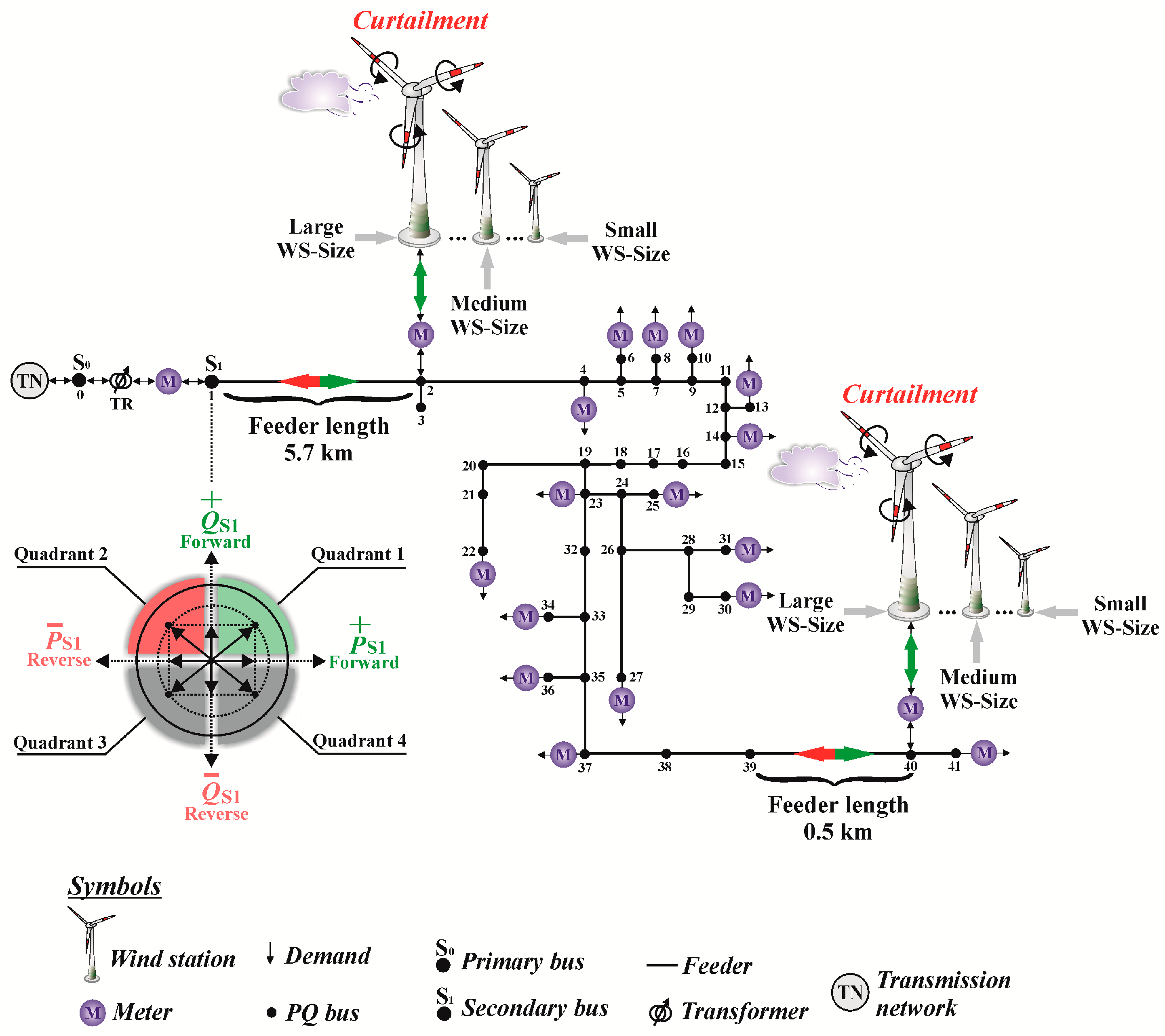The effect of feeder congestion is clearly seen from Table 3 and Table 7 where the costs of reactive energy import F₅ is not totally (i.e., 100%) avoided in the case of the WS-location at bus 40. This is because the WS is located far away from the exporting position S₁ in comparison to the WS located near S₁., i.e., at bus 2.

5.3. The Impact of WS-Size at Bus 2 or Bus 40

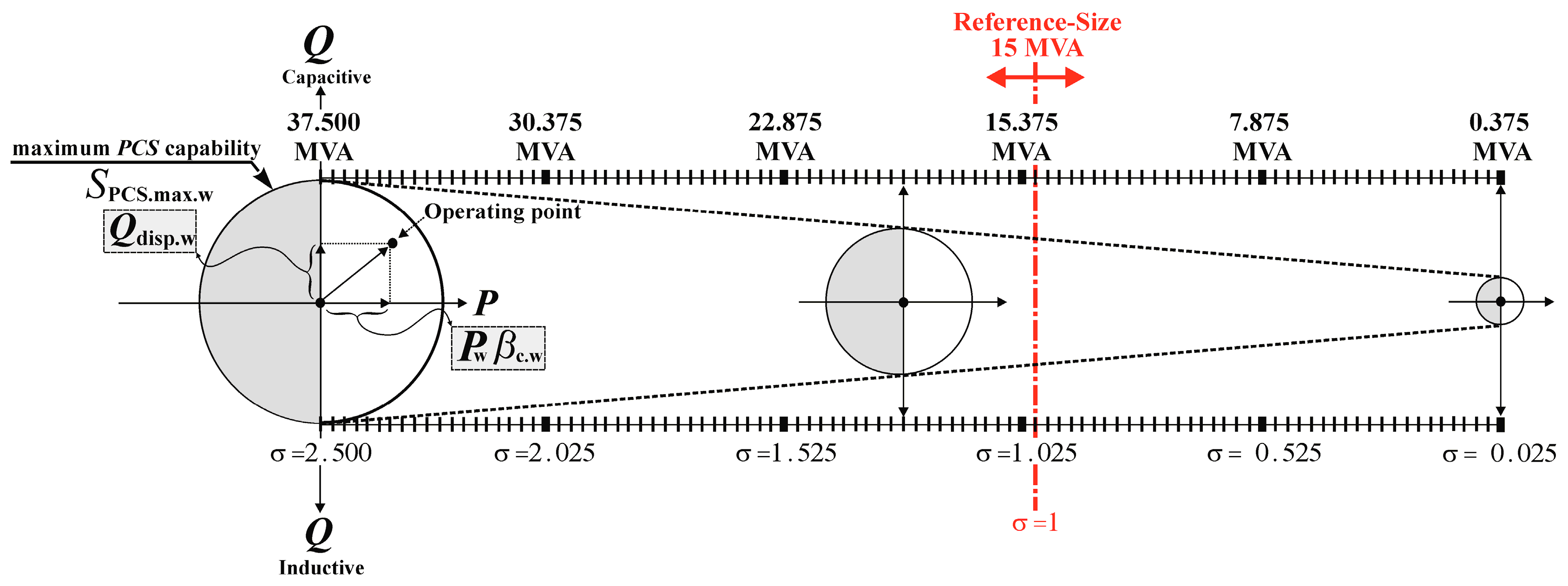
Here, we investigate the impact of the 100 WS-sizes defined in Figure 3 at two WS-locations, namely bus 2 or bus 4, to extract its relations to VRPF. It is aimed to find the maximum feasible WS-size (at a specific location) without violating system constraints. For this reason, the curtailment factor β_c.w is set to 1 in this sub-section, i.e., no wind power curtailment is allowed in all cases as explained above. The results are given in

Table 9. The maximum feasible WS-Size (in MW for P_W and MVA for S_PCS.max.w) according to α_P1.rev at different WS-locations and demand levels.

αP1.rev	0.0	0.1	0.2	0.3	0.4	0.5	0.6	0.7	0.8	0.9	1.0
Bus 2 and 10% demand	0.750	3.0	4.875	6.75	9.0	10.875	13.125	15.0	17.250	19.125	21.375
Bus 40 and 10% demand	0.750	3.0	4.875	7.125	7.5	7.5	7.5	7.5	7.5	7.5	7.5
Bus 2 and 150% demand	15.0	16.875	19.125	21.0	23.25	25.125	27.0	29.250	31.50	32.250	34.125
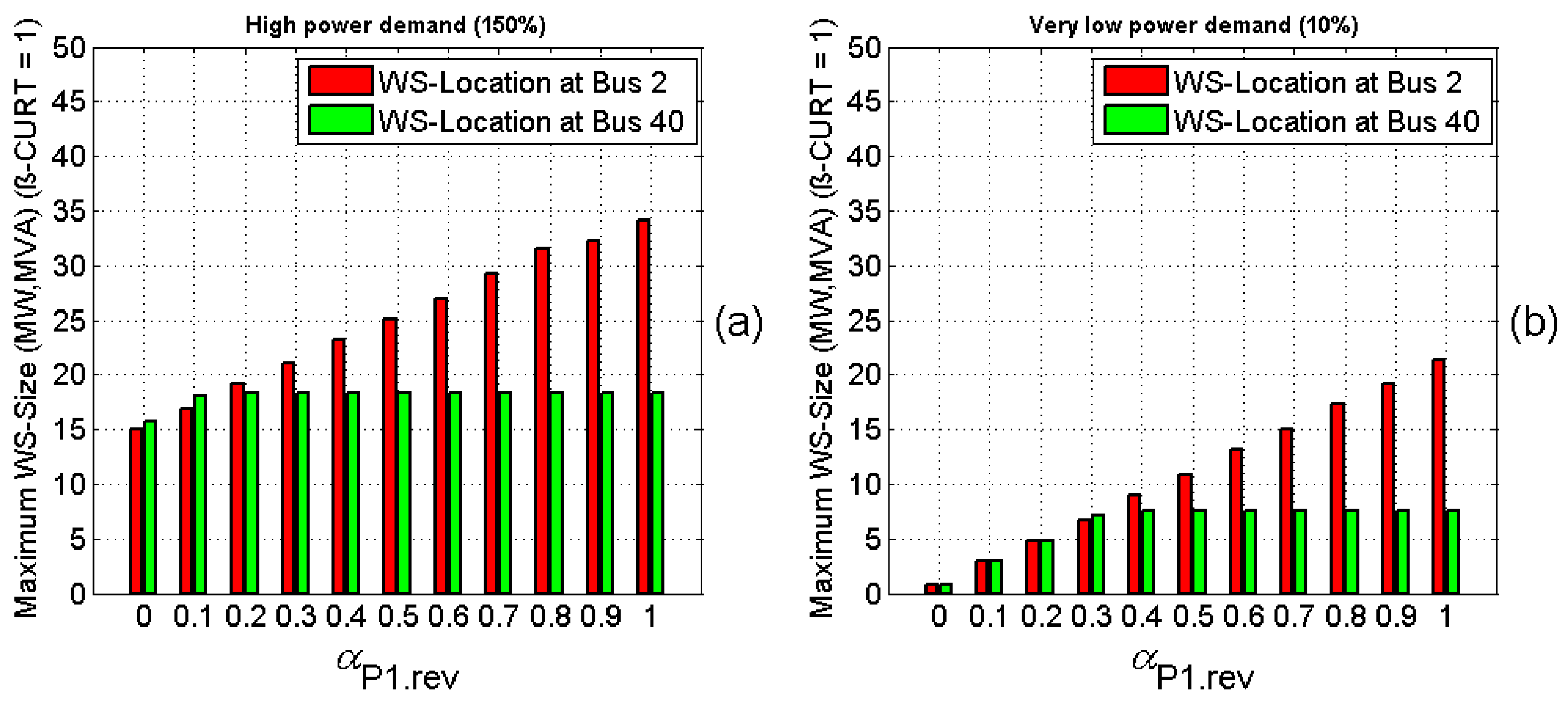
Bus 40 and 150% demand	15.750	18.0	18.375	18.375	18.375	18.375	18.375	18.375	18.375	18.375	18.375

and shown in Figure 8.

The results show clearly how agreed/allowed levels of reverse power flow affect the choice of the maximum feasible WS-size at a defined location. Another important fact is that the demand level in the MV-ADN also plays an important role. For example, if the demand connected to the MV-ADN is high, large WS-sizes will be feasible without any wind power curtailment. In addition, if the HV-TN operator/company agrees to accept the maximum level of reverse energy, i.e., at α_P1.rev = 1, the MV-ADN operator/company will install large WS-sizes. In summary, planning and operating a MV-ADN with high penetration of wind power requires a well-defined agreement for forward/reverse active/reactive power flow from/to the HV-TN.

6. Conclusions

In this paper, we have presented the relationships and the interplay between wind generation curtailment, VRPF, varying PFs of WSs, different demand levels, and active/reactive energy prices in an electricity market model under different scenarios. It is shown that the extended A-R-OPF allows WSs to provide reactive power as, e.g., capacitor banks and battery storage systems. In addition, we derived based on computation results clear rules for power system planners when VRPF is allowed. Moreover, it is shown that reactive reverse power flow will be minimized by using the developed model to avoid any possible charge for reverse reactive energy. Moreover, the reactive power of WSs can be utilized for avoiding extra costs of investments for reactive power provision. Furthermore, optimizing the reactive power flow according to the location of WSs can reduce huge costs, especially in the case of low demand, high wind power generation, and a high level of allowed reverse active power flow. This can be achieved with a well-defined reverse active power flow agreement between different power system operators in electricity markets. Finally, strong relationships between WS-sizes/WS-locations, VRPF and demand level are shown. As a result, the level of allowed reverse power flow will strongly affect the final decision when planning a high penetration of wind power.

References

1. Gabash, A.; Li, P. On variable reverse power flow-part I: Active-Reactive optimal power flow with reactive power of wind stations. Energies 2016, 9. [Google Scholar] [CrossRef]
2. Gabash, A.; Li, P. Variable reverse power flow-part II: Electricity market model and results. In Proceedings of the 2015 IEEE 15th International Conference on Environment and Electrical Engineering (EEEIC), Rome, Italy, 10–13 June 2015; pp. 27–32.
3. ENTSO-E Overview of transmission tariffs in Europe: Synthesis 2015. Available online: https://www.entsoe.eu (accessed on 26 February 2016).
4. Atwa, Y.M. Distribution System Planning and Reliability Assessment under High DG Penetration. Ph.D. Thesis, University of Waterloo, Waterloo, ON, Canada, 2010. [Google Scholar]
5. Gabash, A. Flexible Optimal Operations of Energy Supply Networks: With Renewable Energy Generation and Battery Storage; Südwestdeutscher Verlag: Saarbrücken, Germany, 2014. [Google Scholar]
6. Jayawardena, A.V.; Meegahapola, L.G.; Robinson, D.A.; Perera, S. Microgrid capability diagram: A tool for optimal grid-tied operation. Renew. Energy 2015, 74, 497–504. [Google Scholar] [CrossRef]
7. Arefifar, S.A.; Mohamed, Y.A.-R.I. DG mix, reactive sources and energy storage units for optimizing microgrid reliability and supply security. IEEE Trans. Smart Grid 2014, 5, 1835–1844. [Google Scholar] [CrossRef]
8. Singh, A.K.; Parida, S.K. Novel sensitivity factors for DG placement based on loss reduction and voltage improvement. Electr. Power Energy Syst. 2016, 74, 453–456. [Google Scholar] [CrossRef]
9. Sultana, S.; Roy, P.K. Krill herd algorithm for optimal location of distributed generator in radial distribution system. Appl. Soft Comput. 2016, 40, 391–404. [Google Scholar] [CrossRef]
10. Jordehi, A.R. Allocation of distributed generation units in electric power systems: A review. Renew. Sustain. Energy Rev. 2016, 56, 893–905. [Google Scholar] [CrossRef]
11. Prakash, P.; Khatod, D.K. Optimal sizing and siting techniques for distributed generation in distribution systems: A review. Renew. Sustain. Energy Rev. 2016, 57, 111–130. [Google Scholar] [CrossRef]
12. Stadler, M.; Cardoso, G.; Mashayekh, S.; Forget, T.; DeForest, N.; Agarwal, A.; Schönbein, A. Value streams in microgrids: A literature review. Appl. Energy 2016, 162, 980–989. [Google Scholar] [CrossRef]
13. Soroudi, A.; Siano, P.; Keane, A. Optimal DR and ESS scheduling for distribution losses payments minimization under electricity price uncertainty. IEEE Trans. Smart Grid 2016, 7, 261–272. [Google Scholar] [CrossRef]
14. Sedghi, M.; Ahmadian, A.; Aliakbar-Golkar, M. Optimal storage planning in active distribution network considering uncertainty of wind power distributed generation. IEEE Trans. Power Syst. 2016, 31, 304–316. [Google Scholar] [CrossRef]
15. Kim, S.W.; Kim, J.; Jin, Y.G.; Yoon, Y.T. Optimal bidding strategy for renewable microgrid with active network management. Energies 2016, 9. [Google Scholar] [CrossRef]
16. Garces, A. A quadratic approximation for the optimal power flow in power distribution systems. Electr. Power Syst. Res. 2016, 130, 222–229. [Google Scholar] [CrossRef]
17. IEC 61400–27–1. Wind turbines – Part 27–1: Electrical simulation models –Wind turbines. Edition 1.0, 2015–02; International Electrotechnical Commission: Geneva, Switzerland, 2015. [Google Scholar]
18. Gabash, A.; Xie, D.; Li, P. Analysis of influence factors on rejected active power from active distribution networks. In Proceedings of the IEEE Power & Energy Student Summit, Ilmenau, Germany, 19–20 January 2012; pp. 25–29.
19. Gabash, A.; Li, P. Active-Reactive optimal power flow in distribution networks with embedded generation and battery storage. IEEE Trans. Power Syst. 2012, 27, 2026–2035. [Google Scholar] [CrossRef]
20. Gabash, A.; Li, P. Flexible optimal operation of battery storage systems for energy supply networks. IEEE Trans. Power Syst. 2013, 28, 2788–2797. [Google Scholar] [CrossRef]
21. Gabash, A.; Li, P. Reverse active-reactive optimal power flow in ADNs: Technical and economical aspects. In Proceedings of the 2014 IEEE International Energy Conference (ENERGYCON), Cavtat, Croatia, 13–16 May 2014; pp. 1115–1120.
22. ENERCON Products. Available online: http://www.enercon.de (accessed on 26 February 2016).
23. Vestas Products. Available online: https://www.vestas.com (accessed on 26 February 2016).
24. SIEMENS Wind Power Platforms. Available online: http://www.energy.siemens.com (accessed on 26 February 2016).
Figure 1. The medium-voltage active distribution network (MV-ADN) case study with active-reactive power flow direction definitions and capability diagram of a transformer (TR) at slack bus S1 [5]. Here, different locations and sizes of a wind station (WS) are depicted to show the effect of variable reverse power flow (VRPF).
Energies 09 00235 g001
Figure 2. Simplified model of a WS [1]. Here, M stands for electrical meter and the wind turbine (WT) is connected to the grid through a full scale power converter or power conditioning system (PCS) as in [17] while the wind speed is converted to wind power Pw as in [5].
Energies 09 00235 g002
Figure 3. Illustration of 100 different sizes of a WS. Note that the size of a wind turbine (WT) is considered to be equal to the size of a PCS [1] and the WS-size is considered to be equal to a wind power plant (WPP) [17].
Energies 09 00235 g003
Figure 4. The maximum (a) and minimum (b) voltage amplitude of all buses corresponding to the case study in Table 4. Note 1: the voltage amplitude at slack bus S1 is fixed at 1.02 pu. Note 2: the lower and upper bounds of voltage amplitudes are 0.94 and 1.06 pu, respectively.
Energies 09 00235 g004
Figure 5. Trajectories by the extended and original A-R-OPF based on αP1.rev = 0 (left column) and αP1.rev = 0.5 (right column) at wind power (100%). (a) Wind power generation of the WS (solid-blue) and total demand power (dashed-black); (b) active power dispatch of the WS; (c) reactive power dispatch of the WS; (d) curtailment factor at the WS; (e) slack bus active power; (f) slack bus reactive power; (g) PF of the WS denoted by PFw. Note: from (b) to (g) the lines (dashed-red) stand for the original A-R-OPF (PFmin.w = 1) and (solid-blue) for the extended A-R-OPF (PFmin.w = 0.85).
Energies 09 00235 g005
Figure 6. Trajectories by the extended A-R-OPF based on wind power (50%) (left column) and wind power (0%) (right column) at αP1.rev = 0.5. (a) Wind power generation of the WS (solid-blue) and total demand power (dashed-black); (b) active power dispatch of the WS; (c) Reactive power dispatch of the WS; (d) curtailment factor at the WS; (e) slack bus active power; (f) slack bus reactive power; (g) PF of the WS denoted by PFw. Note: from (b) to (g) the lines (dashed-red) stand for the extended A-R-OPF (PFmin.w = 0.85) and (solid-blue) for the extended A-R-OPF (PFmin.w = 0).
Energies 09 00235 g006
Figure 7. Relationships between (F4 + F5) and αP1.rev at wind power (100%) for the WS at bus 2 (a) or the WS at bus 40 (b). Note 1: the lines (dashed) stand for the original A-R-OPF (PFmin.w = 1) and (solid) for extended A-R-OPF (PFmin.w = 0.85). Note 2: for the demand level, lines (blue) stand for demand (150%), (red) for (100%), (black) for (50%) and (magenta) for (10%). Note 3: the positive values mean costs while negative values mean revenues.
Energies 09 00235 g007
Figure 8. Ilustration of the reseuls in Table 9. Note that all scenarios are carried out at PFmin.w = 0.85, βc.w = 1, high demand (150%) (a) and very low demand (10%) (b).
Energies 09 00235 g008