Abstract
External air movement within built neighborhoods is highly dependent on the morphological parameters of buildings and surroundings, including building height and street cavity ratios. In this paper, computational fluid dynamics (CFD) methods were applied to calculate surface pressure distributions on building surfaces for three city models and two wind directions. Pressure differences and air change rates were derived in order to predict the heating load required to cover heat losses caused by air infiltration. The models were based on typical urban layouts for three cities, and were designed of approximately equal built volumes and equal air permeability parameters. Simulations of the three analyzed building layouts resulted in up to 41% differences in air change rates and heat losses caused by air infiltration. In the present study, wind direction did not have a significant impact on the relative difference between the models, however sideward wind direction caused higher air change rates and heat losses for all simulated layouts.
1. Introduction
Urban morphology parameters, such as urban plan area density, frontal area density, geometry of the buildings, and topographical features influence airflows in and around buildings and, ultimately, energy consumption on a regional scale [1,2]. Airflow patterns in urban areas, referred further as neighborhoods, are especially important for buildings with natural or hybrid ventilation. However, air infiltration, urban heat island formation and airborne pollutant accumulation can affect air quality (IAQ) on the neighborhood or building scale, the coefficient of performance (COP) of heating, ventilation and air conditioning (HVAC) systems, and the heating and cooling demand of mechanically ventilated buildings as well [1]. Spatial arrangement of the neighborhoods influences energy transfer via convection, infiltration and conduction.
Several studies have provided integrated approaches for combining urban airflow simulations with energy performance tools. Indoor-outdoor building energy simulator TUF3D was one of the first three-dimensional fully-coupled indoor-outdoor building energy simulators which allows analysis of urban energy use based on urban geometry, material modifications and the interaction between buildings and their surroundings [3]. Yang et al. established an integrated simulation method capable of quantifying the effects of various microclimatic factors on building energy performance under given urban contexts [4].
Among the many types of energy related interactions between a building and its surroundings, air infiltration can be responsible for a significant portion of a building’s energy consumption, depending on construction and design parameters. It is proved [5] that the time-averaged wind pressure coefficient Cp is one of the best indicators of indoor-outdoor environment interaction due to air infiltration. It is defined as follows:
where px is the static pressure at a given point on the building façade (Pa), p0 is the static reference pressure (Pa), pd is the dynamic pressure, ρ is the air density (kg/m³) and Uref is the reference wind speed at building height h in the windward undisturbed flow (m/s) [5].
Cp values are determined according to orientation and height of the component, building and zone characteristics, shielding and building location [6]. It is common practice to use surface-averaged Cp values for air infiltration and ventilation studies. However, using such values may lead to significant errors in the airflow calculations compared to using local Cp values at the exact coordinates of the building where ventilation equipment is located [5]. This is especially true for natural ventilation cases. Uncertainties of the air change rate calculations can also be increased by neglecting the surroundings of the analyzed buildings or neighborhoods [7].
Van Moeseke et al. demonstrated changes in air flow inside buildings when horizontal as well as vertical pressure coefficient gradients on buildings’ sides are considered [8]. CFD has proven to be an effective tool to predict air movement and air temperature distribution for solving complex problems within urban neighborhoods [9,10]. Experiments and CFD simulations performed by Hang et al. showed different wake flows and even airflow patterns for round and square idealized city models. The overall city form, the configuration of streets and street orientation relative to the approaching wind direction was found to have a great influence on the airflow within the street cavity. Weaker wind was observed in the street network of the square city model than that in the round city model [11]. The interaction of the external wind flow and the internal thermally-driven flow depends upon the ratio of the building height to the urban canyon width [12].
This study is based on the hypothesis that the urban morphology parameters can either increase or decrease wind impacts on buildings, depending on the building type and the aim of urban planners. Actually, heat loss due to air infiltration and leakage depends heavily on a buildings’ plan layout and construction techniques. Modern, airtight and mechanically ventilated buildings are expected to be rather insensitive to wind effects on infiltration so the main focus in this study is on existing buildings without mechanical ventilation, which represent a large portion of the European building stock and even more so in the case of residential buildings. However, apart from the effect of each building’s parameters, the purpose of this study is to implement urban airflow simulations in order to identify the possible effect of urban scale morphology on the potential for infiltration. This is considered as the driving force that interacts with the building scale construction and plan parameters. The pressure distribution on building surfaces was used as an indicator in order to estimate the potential impact of urban morphology on air infiltration and energy use. Three city models, each at two wind directions, were analyzed by means of computational fluid dynamics (CFD) simulations. Air speed and turbulence within the street cavity is examined and used as an indicator of general neighborhood aeration. The results of the simulations showed up to 41% increase in both air change rates and heat losses caused by air infiltration for the analyzed city models. Sideward wind direction resulted in higher overall air change rates for all neighborhoods compared to perpendicular wind direction.
2. Results
2.1. Urban Morphologies Selected for the Study
Two wind directions and three urban morphologies were analyzed in this study, which are further defined as UM-1, UM-2 and UM-3. The morphologies were designed to accommodate approximately the same built volume (600,000 m³) within the same area of the neighborhood (300 m × 300 m) and the surroundings were imitated by placing buildings of a smaller size around the main domain of interest. The geometry of the surrounding buildings was the same for all cases. The morphology of the analyzed regions was designed according to layouts of real cities, namely Zürich (Switzerland), Kaunas (Lithuania) and Athens (Greece). The geometries and views of the cities they represent are provided in Figure 1.
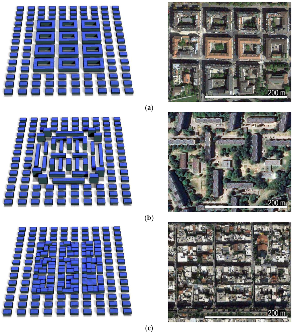
Figure 1.
Urban morphologies with uniform surrounding buildings used for CFD analysis in comparison to the real city images: (a) UM-1—Zürich, Switzerland; (b) UM-2—Kaunas, Lithuania; (c) UM-3—Athens, Greece. Map data ©2015 Google.
The real city layouts and building heights were modified to satisfy the requirements of equal built volumes and neighborhood area. The building heights, average building height and street cavity width ratios used for the simulations are presented in Table 1.

Table 1.
Height of buildings and its ratio to street width for selected urban morphologies.
Pressure differences on building surfaces were used to predict air infiltration and the potential impact on energy consumption due to air infiltration in the built neighborhood. Detailed descriptions of the simulation methods, validation of the CFD model and calculation procedures are provided in the Methods section.
2.2. CFD Prediction Results for Air Speed and Building Surface Pressure Distribution
CFD predictions proved the hypothesis that urban morphology is a critical factor, significantly affecting pressure distribution on building surfaces (Figure 2), which in turn determines the pressure differences that drive infiltration. Results of the simulations with perpendicular wind (0°) revealed that the highest pressure differences appear on the windward side building surfaces for morphologies UM-1 and UM-3. However, higher buildings (up to 36 m) were present in UM-2 case, and therefore, relatively high pressure differences on the leeward building surfaces were observed as well. Effects of irregularities of building heights can also be observed in UM-3 cases. CFD predictions proved the hypothesis that urban morphology is a critical factor, significantly affecting pressure distribution on building surfaces (Figure 2), which in turn determines the pressure differences that drive infiltration. Results of the simulations with perpendicular wind (0°) revealed that the highest pressure differences appear on the windward side building surfaces for morphologies UM-1 and UM-3. However, higher buildings (up to 36 m) were present in UM-2 case, and therefore, relatively high pressure differences on the leeward building surfaces were observed as well. Effects of irregularities of building heights can also be observed in UM-3 cases.
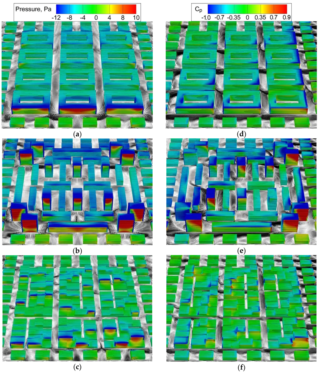
Figure 2.
CFD prediction results of air pressure and wind pressure coefficient distribution on building surfaces and air speed vectors at the height of 2 m: (a,d) Urban morphology UM-1; (b,e) Urban morphology UM-2; (c,f) Urban morphology UM-3; (a–c) Perpendicular wind direction; (d–f) Sideward wind direction, 45°.
Air speed contours at three heights (2 m, 10 m and 15 m) and turbulent kinetic energy contours at 10 m height for both wind directions are provided in the Supplementary Materials of this paper as Figures S1 and S2, respectively.
Also shown in Figure 2 is a scale of the commonly used wind pressure coefficient (1). As the buildings of different heights are present in different models, the reference velocity has been taken at 10 m height i.e., Uref = 4.5 m/s. It can be observed from Figure 2a,d that homogeneous urban morphology resulted in better wind shading effects. Highest pressure differences were present on surfaces of the buildings located on the windward side (UM-1). On the other hand, irregularities in building heights caused higher pressure differences on the leeward building surfaces for UM-2 and UM-3 cases. In the street canyons, higher values for turbulent kinetic energy were observed for UM-2 and UM-3 models, although air speed within the neighborhood was the highest for the UM-1 model.
2.3. Results of Air Infiltration and Expected Impact on Energy Consumption Calculations
Pressure differences on building surfaces were obtained by post-processing the CFD simulation results. The obtained values are presented in Figure 3 (median values, inter-quartile range as well as minimum and maximum values). The highest standard deviation and range of values were obtained for urban morphology UM-2 at both wind directions. As can be observed from Table 2, this layout also resulted in the highest air change rates and energy consumption required to cover air infiltration heat losses, subject to assumptions for leakage area and discharge coefficient.
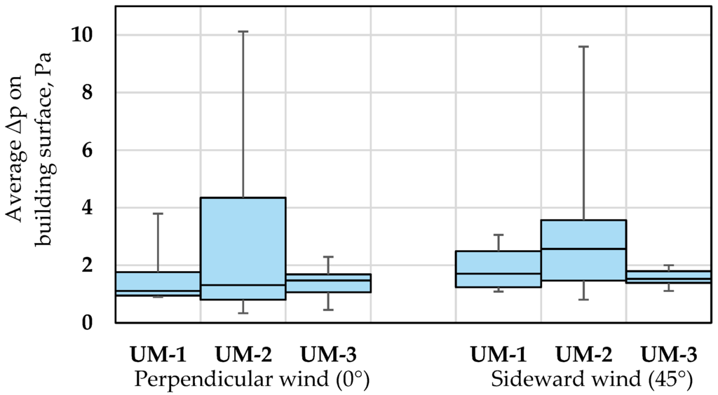
Figure 3.
Pressure difference (Δp) distribution on building surfaces for urban morphologies UM-1, UM-2, UM-3 and two wind directions (0° and 45°). Horizontal lines within bars indicate median values, bars denote inter-quartile ranges and whiskers define the full range of values.
Table 2.
Results of air infiltration and expected impact on energy consumption calculations.
In Table 2, both weighted Δp values and weighted air change rates were calculated considering the volume of buildings. In all cases, potential heat losses were estimated by Equation (6), presented in the Section 4.4 by using the same typical 10 K air temperature difference between indoors and outdoors. In Table 2 heat losses are presented for the whole analyzed neighborhood. The results of this study prove that urban morphology has a significant impact on air infiltration and air movement within street cavities.
With regard to energy demand, this impact may or may not be significant, depending on other factors such as airtightness, building plan depth etc. The results presented here refer to the change in relative energy consumption due to infiltration alone. The following conclusions can be drawn:
- The highest values of average speed and the lowest for turbulent kinetic energy within street cavities were observed in the case of urban morphology UM-1. However, it seems that this layout exhibits better aerodynamic properties that allow a reduction of wind induced energy consumption by approx. 41% compared to urban morphology UM-2. Therefore, designing built neighborhoods according to this overall spatial shape should be considered to achieve lower energy consumption of smart cities.
- The highest wind induced air change rates and pressure differences on building surfaces were observed for urban morphology UM-2. Mixed building height and highest average building height and street width ratio resulted in a significant increase of the estimated heat load required to cover the heat losses despite the wind direction.
- A relatively small difference between the results of the layouts UM-1 and UM-3 was found. These models however, were similar in that buildings were joined into blocks in both cases. This leads to overall lower values of air leakage areas as, in this study, air leakage areas were calculated from specific leakage area (AL, cm2/m2) according to the exposed surface areas of the buildings.
3. Discussion
This study focused on finding relative differences of air change rates and energy consumption caused by wind effects for different urban layouts. Therefore, isothermal conditions were simulated by means of CFD and the stack effect was neglected as a driving force. This assumption is not expected to influence the results and conclusions since pressure effects on infiltration rates are additive [13]. Air change rates were estimated by using differential pressure on building surfaces as an input and considering similar air leakage area per total surface area of the buildings for all cases. Inclusion of the stack effect would be more realistic, but under the relatively high wind speed being examined, the wind induced pressure difference is expected to be the dominant mechanism. Furthermore, inclusion of the stack effect would increase the number of degrees of freedom for the design of the numerical experiment, such as indoor-outdoor air temperature difference and air leakage within the buildings itself.
It is also worth noting that urban morphologies analyzed in this study were selected as representative cases for Northern, Central and Southern Europe and were only used to build the initial geometries. The simulations were carried out with the same wind profiles used to define boundary conditions and the same temperature difference of 10 K was used for heating load calculations. The results should therefore be interpreted in a way that optimal solution might be different depending on the geographical location of the neighborhood. Higher values of air speed within the street cavities can be chosen as a goal while planning neighborhoods in warm climates and the aim to reduce pressure differences on building surfaces can be adopted for cold climate cities.
4. Methods
4.1. Urban Morphologies and Boundary Conditions
Three urban morphologies were analyzed in this study. Details of the models UM-1, UM-2 and UM-3 are provided in Section 2.1. The analyzed built neighborhood was surrounded by buildings of a smaller height. The width, length and height of the overall solution domain for UM-1 and UM-3 cases was 750 m × 750 m × 125 m. In UM-2 case, buildings of 36 m were present in the model, therefore the domain was extended to 750 m × 800 m × 180 m. The wind profile was assumed to correspond to neutral atmospheric stability and followed a log-law:
with a roughness length of zo = 0.5 m and the Von Karman constant κ = 0.41. The friction velocity u* was calculated by considering wind speed equal to 4.5 m/s at the height of 10 m and the full profile is presented in Figure 4. A Cartesian grid was adopted with a vertical discretization of 1 m up to a height equal to two building heights above ground and a horizontal discretization of 2 m (width and length). The size of the grid cells was increased closer to the boundaries of the domain. Total number of grid cells varied between 5.2 million (UM-1 and UM-3) and 9.2 million (UM-2). An example of the generated grid for UM-2 case is presented in Figure 5.
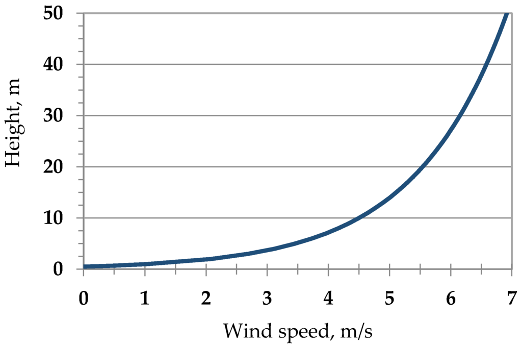
Figure 4.
Wind profile used for CFD simulations.
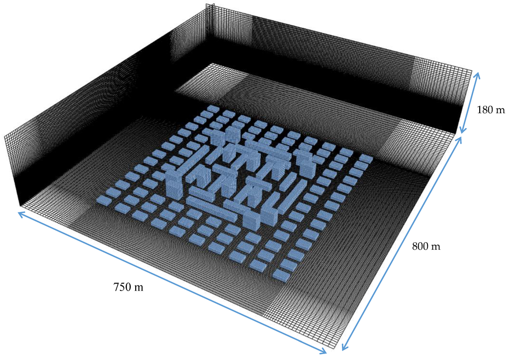
Figure 5.
Example of the calculation grid used for CFD simulations (UM-2 case).
4.2. Tools and Procedures Used for CFD Simulations
Geometries for the CFD models were created through 3D design software (Sketchup, 2015, Trimble Navigation, Ltd., Sunnyvale, CA, USA) and then processed using an in-house algorithm for the definition of solid regions on a Cartesian grid. Sufficient distance from the computational domain boundaries ensured minimal blockage and boundary effects. The numerical modeling involved solution of the 3D volume averaged Reynolds equations with SIMPLE algorithm for pressure velocity coupling [14] and the Rhie and Chow corrections [15] for the collocated grid arrangement. A bounded second order upwind discretization scheme was used for the convective terms and central differences for the rest.
The k-ε turbulence model with wall functions was used for turbulence modeling [16]. The profiles for turbulence kinetic energy and its dissipation rate were calculated assuming local equilibrium [17]:
where is the friction velocity, κ is the von Karman constant (=0.40–0.42) and Cμ is a model constant of the standard k-ε model (=0.09). The velocity and turbulence quantities were considered constant along the top of the computational domain. These boundary conditions correspond to neutral atmospheric conditions and a moderately rough upstream fetch and are in accord with the COST 732 guidelines for CFD simulation of flows in urban environments [18]. Tecplot 360 EX software was used for visualization of the CFD results (2015, Tecplot, Inc., Bellevue, WA, USA).
4.3. Validation of the CFD model
Validation of the CFD methodology in the prediction of surface pressure distribution has been performed in the previously published studies dealing with the flow past a single building [19,20]. The solution domain was extended in this study to a neighborhood scale. Therefore, validation of the computational methodology was performed through a simulation of the experimental study by Davidson et al. [21]. This study was selected for the validation of the model due to well documented boundary conditions, including upstream wind profiles. Staggered array configuration of building imitating cubes were analyzed with the distance between the blocks double the building height. During the wind tunnel experiments, both vertical and horizontal air velocity profiles were measured at X and Y axis by means of pulsed-wire and hot-wire anemometers in between the street cavities. The study demonstrated the reduction in magnitude of the velocity within the array including the far-wakes of individual obstacles spreading and merging with those of neighboring obstacles, reducing the mean flow through the array [21].
Similar boundary conditions were used as an input for CFD simulations. The geometries of the model and the comparison of the velocity profiles are presented in Figure 6. Air velocity profiles are presented at the same coordinates as documented by Davidson et al. and horizontal profiles along the X axis are compared within the same region of interest, excluding the areas shaded in Figure 6.
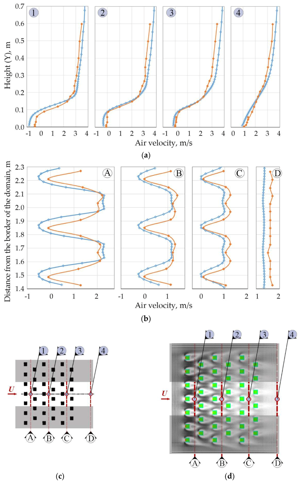
Figure 6.
Vertical (a) and horizontal (b) air velocity profiles obtained by the CFD validation model (d) based on the wind tunnel study (c) by Davidson et al. [21] (  wind tunnel experiment results,
  CFD prediction results).
wind tunnel experiment results, CFD prediction results).
As it can be observed from Figure 6a,b, vertical profiles obtained from CFD simulations were in good agreement with the experimental results. Horizontal profiles indicated that CFD tends to overestimate the building impact on the flow and shows slightly faster reduction in magnitude of the velocity deeper within the building array. However, considering that the main aim of this study was to observe differences between the models, the level of agreement between the models was considered satisfactory. Surface pressure distribution was not measured by Davidson et al., but given the strong relation between pressure distribution on building surfaces and air velocity patterns within street cavities, as well as the previous validation studies for pressure distributions on single buildings [19,20], the computational model’s performance was considered adequate in order to proceed with the present study.
4.4. Air Infiltration Estimation
The technique of equivalent leakage area (ELA) was adopted to obtain the volume flow rates resulting from pressure differences on building surfaces. It is important to note, that stack effect in buildings was not considered in this study and the air change rates were assumed to be generated solely by wind as a driving force. However, the (ELA) technique is based on overall pressure differences between the interior and the exterior of the building and calculation based on detailed local surface pressures is not straightforward. Here, air change rate caused by wind was calculated based on the assumption that the building’s inner pressure is determined by the mean pressure on its exposed surfaces. Therefore, infiltration and exfiltration are determined by independently calculating the positive and negative differences of the local external surface pressure to the building’s inner pressure. The following steps were performed during post processing:
- Reading the pressure values for each grid cell of the building’s exposed surfaces obtained by CFD, and calculating the surface weighted mean external pressure. This defines the building’s inner pressure.
- Determining overall pressure difference by using the difference between the sum of the values which are higher than the inner pressure on the building surface, indicating air infiltration and the sum of the values which are lower than the inner pressure, indicating exfiltration.
- The pressure difference thus obtained was used for calculating the air flow rate by applying the ELA equation [22]:where: Q—air flow rate, m³/h; Cd—the discharge coefficient (0.6 value was used in this study), A—equivalent leakage area, m²; Δp—pressure difference across building surface, Pa (obtained within the step 2); ρ—air density. In this study the values were used as follows:
- Discharge coefficient—0.6 (i.e., the discharge coefficient for a sharp-edged orifice) [13];
- Equivalent leakage area was calculated by using the specific leakage area i.e., the ratio of (AL) and exposed surface area of the building. This ratio was considered 4 cm² per 1 m² of the building surface area [23];
- Air density—1.16 kg/m³.
- Building air change rate was calculated as follows:where: Q—air flow rate, m³/h (obtained within the step 3), volume of the building, m³.
- The total energy consumption of the built neighborhood was estimated by calculating total air flow rates using the average built volume between the simulated cases and air change rates of each particular case. Heating load required to cover air infiltration heat losses was calculated as follows [13]:where: q—sensible heat load, W; Q—air flow rate, m³/s; ρ—air density, kg/m³; cp—specific heat of air, J/kgK; Δt—temperature difference between indoors and outdoors, K.q = ΣQ·ρ·cp·Δt
10 K air temperature difference between indoors and outdoors was used for this study as an estimate of average air temperature difference during the heating season. Example of the infiltration induced air change rate and heating load calculation results are presented for one example building in Appendix A.
Supplementary Materials
The following are available online at www.mdpi.com/1996-1073/9/3/177/s1. Figure S1: Air speed contours at three heights (2 m, 10 m and 15 m) and turbulent kinetic energy contours at 10 m height for perpendicular wind direction (0°) and: (a) UM-1; (b) UM-2; (c) UM-3, Figure S2: Air speed contours at three heights (2 m, 10 m and 15 m) and turbulent kinetic energy contours at 10 m height for sideward wind direction (45°) and: (a) UM-1; (b) UM-2; (c) UM-3.
Acknowledgments
This paper was supported by COST (European Cooperation in Science and Technology) by a STSM Grant from COST Action TU1104 “Smart Energy Regions“.
Author Contributions
The authors contributed equally to this work. CFD code and post processor used for this study was developed by Demetri G. Bouris; Andrius Jurelionis and Demetri G. Bouris conceived and designed the simulation cases and post processing tools; Demetri G. Bouris performed CFD calculations; Andrius Jurelionis and Demetri G. Bouris analyzed the data; Andrius Jurelionis wrote the paper.
Conflicts of Interest
The authors declare no conflict of interest. The founding sponsors had no role in the design of the study; in the collection, analyses, or interpretation of data; in the writing of the manuscript, and in the decision to publish the results.
Abbreviations
The following abbreviations are used in this manuscript:
| CFD | Computational fluid dynamics |
| ELA | Equivalent Leakage Area |
| IAQ | Indoor air quality |
| UM | Urban morphology |
Appendix A
In this appendix, the results of air change rate and infiltration induced energy consumption calculation for a single building are presented. The building on the windward side of 36 m height was extracted from urban morphology UM-2 (perpendicular wind direction case, 0°).
The location of the building within the neighborhood and CFD simulation results of pressure distribution on building surfaces are presented in Figure A1. The results of the calculations are presented in Table A1 and follows the structure described in Section 4.4.
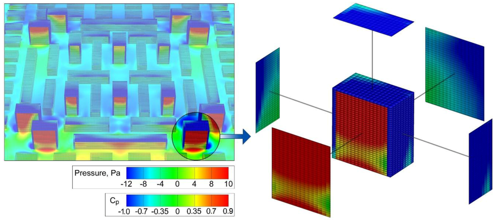
Figure A1.
Air pressure distribution and wind pressure coefficient distribution on the surfaces of one building (UM-2 case, perpendicular wind), used as an example.
Table A1.
Steps and results of air change rate and heat losses calculations for the example building.
| Step | Description and Known Values | Values Obtained | ||
|---|---|---|---|---|
| 1-2 | Calculating the mean pressure on building surfaces and determining the pressure difference | (p-pavg) > 0 = 6.88 Pa (p-pavg) < 0 = –3.24 Pa | Δp = 10.12 Pa | |
| 3 | Air flow rate calculation | Building volume—20979 m³ Air leakage area—1.69 m² | Q = 15222 m³/h | |
| 4 | Building air change rate calculation | ACH = 0.726 | ||
| 5 | Heating load required to cover air infiltration heat losses at Δt = 10 K | q = 40.3 kW | ||
References
- Srebric, J.; Heidarinejad, M.; Liu, J. Building neighborhood emerging properties and their impacts on multi-scale modeling of building energy and airflows. Build Env. 2015, 91, 246–262. [Google Scholar] [CrossRef]
- Rasheed, A.; Robinson, D.; Clappier, A.; Narayanan, C.; Lakehal, D. Representing complex urban geometries in mesoscale modeling. Int.J. Climatol. 2011, 31, 289–301. [Google Scholar] [CrossRef]
- Yaghoobian, N.; Kleissl, J. An indoor–outdoor building energy simulator to study urban modification effects on building energy use—Model description and validation. Energy Build 2012, 54, 407–417. [Google Scholar] [CrossRef]
- Yang, X.; Zhao, L.; Bruse, M.; Meng, Q. An integrated simulation method for building energy performance assessment in urban environments. Energy Build 2012, 54, 243–251. [Google Scholar] [CrossRef]
- Cóstola, D.; Blocken, B.; Ohba, M.; Hensen, J.L.M. Uncertainty in airflow rate calculations due to the use of surface-averaged pressure coefficients. Energy Build 2010, 42, 881–888. [Google Scholar] [CrossRef]
- EUROPEAN STANDARD STORE. Ventilation for Buildings—Calculation Methods for the Determination of Air Flow Rates in Buildings Including Infiltration; EUROPEAN STANDARD STORE: Pilsen, Czech Republic, 2007. [Google Scholar]
- Van Hooff, T.; Blocken, B. On the effect of wind direction and urban surroundings on natural ventilation of a large semi-enclosed stadium. Comput. Fluid. 2010, 39, 1146–1155. [Google Scholar] [CrossRef]
- Van Moeseke, G.; Gratia, E.; Reiter, S.; De Herde, A. Wind pressure distribution influence on natural ventilation for different incidences and environment densities. Energy Build 2005, 37, 878–889. [Google Scholar] [CrossRef]
- Ramponi, R.; Blocken, B.; de Coo, L.B.; Janssen, W.D. CFD simulation of outdoor ventilation of generic urban configurations with different urban densities and equal and unequal street widths. Build Env. 2015, 92, 152–166. [Google Scholar] [CrossRef]
- Toparlar, Y.; Blocken, B.; Vos, P.; van Heijst, G.J.F.; Janssen, W.D.; van Hooff, T.; Montazeri, H.; Timmermans, H.J.P. CFD simulation and validation of urban microclimate: A case study for Bergpolder Zuid, Rotterdam. Build Env. 2015, 83, 79–90. [Google Scholar] [CrossRef]
- Hang, J.; Sandberg, M.; Li, Y. Effect of urban morphology on wind condition in idealized city models. Atmos Env. 2009, 43, 869–878. [Google Scholar] [CrossRef]
- Syrios, K.; Hunt, G.R. Passive air exchanges between building and urban canyon via openings in a single façade. Int. J. Heat Fluid Flow 2008, 29, 364–373. [Google Scholar] [CrossRef]
- ASHRAE TC 4.3. Ventilation and infiltration. In ASHRAE Handbook-Fundamentals; American Society of Heating, Refrigerating and Air-Conditioning Engineers, Inc. (ASHRAE): Atlanta, GA, USA, 2013.
- Patankar, S.; Spalding, D. A calculation procedure for heat, mass and momentum transfer in three dimensional parabolic flows. Int. J. Heat Mass Transf. 1972, 15, 1787–1806. [Google Scholar] [CrossRef]
- Rhie, C.; Chow, W. Numerical study of the turbulent flow past an airfoil with trailing edge separation. AIAA J. 1983, 21, 1525–1532. [Google Scholar] [CrossRef]
- Launder, B.E.; Spalding, D.B. The numerical computation of turbulent flows. Comput. Method. Appl. Mech. Eng. 1974, 3, 269–289. [Google Scholar] [CrossRef]
- Blocken, B.; Stathopoulos, T.; Carmeliet, J. CFD simulation of the atmospheric boundary layer: Wall function problems. Atmos Env. 2007, 41, 238–252. [Google Scholar] [CrossRef]
- Franke, J.; Hellsten, A.; Schlünzen, H.; Carissimo, B. Best Practice Guideline for the CFD Simulation of Flows in the Urban Environment, COST Action 732 Quality Assurance and Improvement of Microscale Meteorological Models; Meteorological Institute: Hamburg, Germany, 2007. [Google Scholar]
- Barmpas, F.; Bouris, D.; Moussiopoulos, N. 3D Numerical simulation of the transient thermal behaviour of a simplified building envelope under external flow. J. Sol. Energy Eng. 2009, 131. [Google Scholar] [CrossRef]
- Petridou, M.; Bouris, D. Experimental and numerical study of the effect of openings on the surface pressure distribution of a hollow cube. WSEAS Trans. Fluid Mech. 2006, 1, 655–662. [Google Scholar]
- Davidson, M.J.; Snyder, W.H.; Lawson Jr, R.E.; Hunt, J.C.R. Wind tunnel simulations of plume dispersion through groups of obstacles. Atmos. Env. 1996, 30, 3715–3731. [Google Scholar] [CrossRef]
- ATTMA. Technical standard 1. Measuring Air Permeability of Building Envelopes, Air Tightness Testing and Measurement Association. Available online: http://www.attma.org (accessed on 1 October 2015).
- Urquhart, R.; Richman, R.; Finch, G. The effect of an enclosure retrofit on air leakage rates for a multi-unit residential case-study building. Energy Build 2015, 86, 35–44. [Google Scholar] [CrossRef]
© 2016 by the authors; licensee MDPI, Basel, Switzerland. This article is an open access article distributed under the terms and conditions of the Creative Commons by Attribution (CC-BY) license (http://creativecommons.org/licenses/by/4.0/).