Distributed Renewable Generation and Storage System Sizing Based on Smart Dispatch of Microgrids

Abstract

This paper considers the contribution of independent owners (IOs) operating within microgrids (MGs) toward green power generation in deregulated energy markets. An optimization scheme is introduced for sizing distributed renewable generation (DRG) and a distributed energy storage system (DESS) based on a novel energy management system (EMS) that accounts for demand response (DR), DESS dispatch and performance degradation, dynamic pricing environments, power distribution loss and irregular renewable generation. The proposed EMS utilizes an iterative Newton-Raphson linear programming algorithm that schedules resources in order to minimize the objective function, to deal with the complicated nonlinear nature of the problem and to enable efficient long-term assessments. The EMS is used to evaluate candidate solutions that are generated by a genetic algorithm (GA) to determine the optimal combination of DRG and DESS. A case study for IEEE 34-bus distribution MG in Okinawa, Japan, is used for testing the algorithm and analyzing the potential for IO/MG investments and their strategies.

1. Introduction

Meeting electricity demand, with its accelerated growth, is one of the biggest economic and environmental challenges facing developing nations. For this reason, distributed generation (DG) has been introduced to supply power at the distribution level, reducing the dependence on centralized power generation and improving the transmission and distribution efficiency. DG uses fossil fuels, such as diesel and gas gensets, or renewable sources, such as photovoltaics (PVs) and wind turbines (WTs).

The problem of planning a DG-integrated power system has attracted significant attention, and a large amount of literature exists [1,2,3,4,5,6,7,8,9,10,11,12,13,14,15,16,17,18,19,20,21,22]. For example, a model for allocating and sizing DG that intends to minimize the total investment, operating and substation and feeder upgrade costs was proposed in [14]. The work in [1] proposed allocating DG in deregulated energy markets based on the locational marginal price of the network nodes. The work in [8] introduced a novel model for maximizing utility profits while guaranteeing payback to the DG owner within a certain period to boost private sector participation in deregulated electricity markets, which are more efficient and competitive than regulated markets. Although the majority of the aforementioned studies considered power supply security constraints, the main objectives of some studies were to maximize power reliability and supply adequacy, as in [13], which proposed the integration of a mix of DG, reactive resources and distributed energy storage systems (DESSs) into a modern power system within the microgrid (MG) operation framework. The ability to partly curtail and shift heat, air ventilation, and cooling (HAVC) load was highlighted during the planning stage in [23]. Some studies discussed the problem by considering uncertain consumption patterns due to the stochastic control of electric vehicles (EVs) and uncertain distributed renewable generation (DRG) due to weather conditions [10]. As the smart grid concept rapidly evolves and finds increased acceptance while reshaping the conventional power system, attention should be paid to account for the electric consumption flexibility offered by demand response (DR) programs. However, the impact of DR and smart storage dispatch on the problem has not been properly addressed in the literature. Thus, more extensive studies are required in this area.

Optimization methods vary based on the objective and nature of the problem. In fossil-fuel-based DG, a nonlinear programming optimization can be used; it is usually performed over a short time horizon [7]. However, in the case of DRG and DESSs, because of daily and seasonal variability, a much longer time horizon must be considered. Because nonlinear programming methods are not computationally efficient on a longer time scale, generally, heuristic optimization methods are used. For example, in [12], a fuzzy particle swarm optimization method was introduced for DESS sizing in order to mitigate the bid risk of wind generator owners. A method that utilizes tribal particle swarm optimization and ordinal optimization coupled with non-linear programming for effectively obtaining optimal and near-optimal solutions was proposed in [24]. A procedure for utilizing the strength of parallel computing in power system planning was presented in [6]. A good review of this problem can be found in [25].

As Japan plans to deregulate its electricity market and significantly boost its share of renewable generation, in-depth studies are required to estimate the potential contribution of small- to mid-scale independent owners (IOs) toward the green electricity market for determining encouraging pricing strategies. These systems can also be installed by the MG community by using long-term loans; however, their design and operation are different for each case; a system owned by an MG will be operated in order to reduce the power supply cost. In contrast, IOs always seek to maximize their own profit. This study proposes a model for sizing DRG and DESSs based on these two goals and fulfilling the following targets:

• An integrated and comprehensive model that accounts for DR, DESS dispatch and performance degradation, dynamic pricing environments, power distribution loss and irregular renewable generation.
• Intelligent energy management that coincides with a smart grid framework.
• A computationally-efficient optimization method that can be practically used for long-term planning.

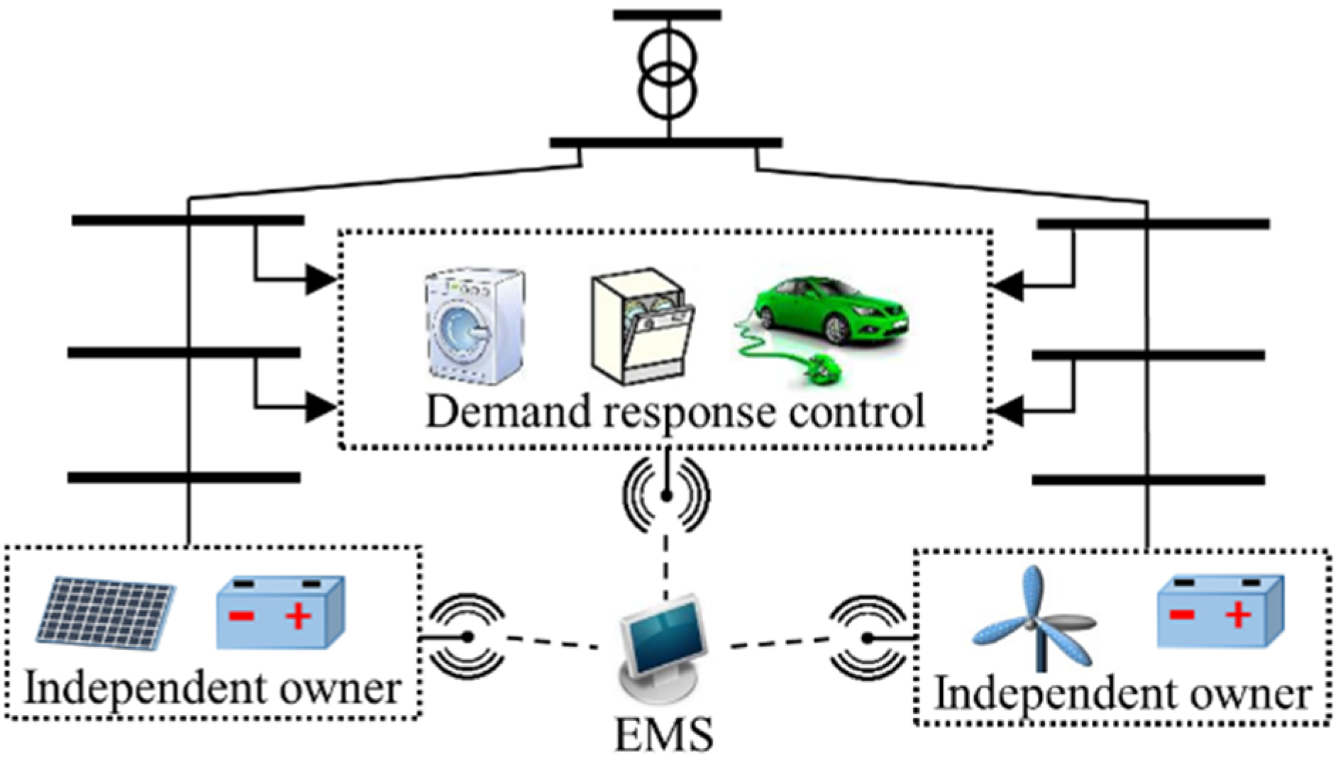
The energy management in MGs can be complicated and challenging, and therefore, many studies proposed suitable solutions that utilize various optimization methods, such as mathematical optimization [26,27], dynamic programming [28] and heuristic-based algorithms [29,30]. Although these methods proved to be accurate and efficient for short-term scheduling and real-time applications, applying them to our problem for long-term assessments in which hundreds or thousands of different combinations of DRG and DESS must be evaluated is not computationally efficient. For this reason, the current study proposes a novel and efficient energy management system (EMS) to tackle the aforementioned challenges when simulating optimal off-line control of an MG in real-world daily operation scenarios on a long-term basis (one year or more). The proposed EMS utilizes an iterative Newton-Raphson linear programming (NRLP) algorithm that iteratively schedules resources in order to minimize the objective function while compensating for the complicated nature of the problem and efficiently performing long-term assessments. The main merit of the proposed EMS is that it enables the usage of efficient linear programming (LP) solvers rather than non-linear programming solvers. At the same time, the algorithm can address distribution power flow and loss, which requires non-linear formulation, through the dispatching process. The EMS is used to evaluate candidate solutions that are generated by a genetic algorithm (GA) to obtain an optimal combination of DRG and DESSs. A case study for IEEE 34-bus distribution MG in Okinawa, Japan, is used for testing the algorithm and analyzing the potential investments of IOs/MG and their strategies.

2. System Structure

In deregulated energy markets, the price of energy depends on supply and demand, as in any other market. A wholesale spot market is widely used to trade electricity; in this market, a wide variety of competitive generators and retailers bid to sell and buy a certain amount of power at certain prices. Then, the retailers re-price the electricity and sell it to consumers. In this study, as shown in Figure 1, it is assumed that each MG acts as one entity, establishing a contract with retailers to buy electricity through the substation at quadratically increasing rates. This function is commonly used because it coincides with the quadratic fuel-consumption function of thermal generation units [31,32] and the increased cost of power generation under high demand met by other fast-response (but less efficient) peaking power plants. This pricing model is also used to stimulate DR programs to shift controllable loads from on-peak to off-peak times [33,34]. Additionally, it is assumed that the MG buys electricity from independent DRG and DESS owners operating within the MG distribution system at the same real-time rates offered by retailers (i.e., the grid). The participation of IOs will reduce the power demanded at the substation and, accordingly, the energy cost. Typically, in such a free market, a decentralized EMS is used, i.e., dynamic pricing is used to stimulate the responses of consumers and IOs. Therefore, several levels of coordinated control are required. In this study (for simplicity), an aggregated EMS to manage and dispatch all available resources to maximize the profit of IOs is considered. At the same time, this EMS considers the consumers’ tendency to reduce their energy consumption bills by using DR control.

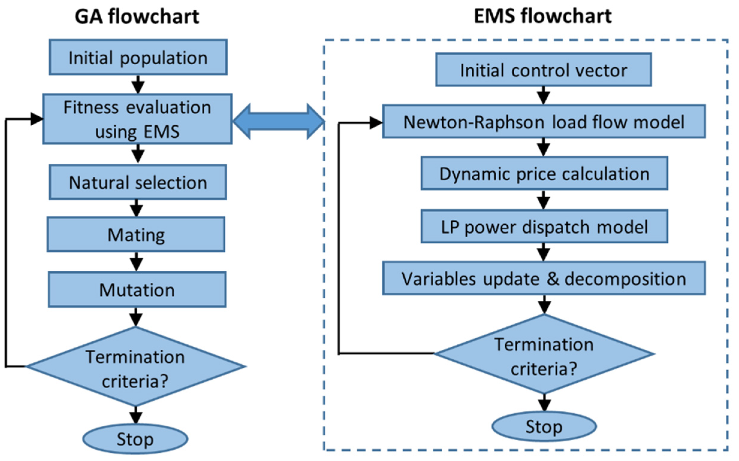
3. Energy Management System

The proposed optimization framework, shown in Figure 2, employs a GA that is dedicated to optimizing the physical structure of the system, i.e., the size of DRG and DESS. In such an algorithm, different potential solutions (DRG and DESS combinations) are evaluated using an EMS and ranked based on their fitness. Therefore, an efficient EMS is required to simulate the daily power dispatching strategies of such solutions over a period of one year to predict the associated annual profits.

The proposed EMS utilizes an iterative NRLP dispatch algorithm. The first step of the algorithm is initializing a dispatch control vector by setting DESS charge/discharge to zero for all hours and randomly distributing the controllable load or scaling it to the expected non-controllable load. Then, a Newton-Raphson load flow (NRLF) procedure is used to evaluate the associated distributed power flow and loss in the MG and the purchased power from the main grid (through the substation) at each hour. Using this procedure, the dynamic prices are calculated. Then, the power dispatch quantities, i.e., the storage charge/discharge power and the shiftable load at each bus of the MG, are aggregated and fed into an LP power dispatch model that is performed for a five-day time window at once in order to adjust the aggregated control vector to a more profitable position. In the final step, the objective function of the operation performance is evaluated; in this step, the algorithm terminates the loop if the objective peak is reached. Otherwise, the algorithm returns to the NRLF step after decomposing the aggregated dispatch vector. After planning the first five-day time window, the algorithm moves to the next time window, and the process continues until the data for one year are simulated. Thus, the annual profit of the system can be predicted. It can be seen clearly that the EMS takes into account the effect of power distribution loss without using general non-linear programming solvers to model the power flow in the feeder to avoid complicating the optimization process.

3.1. Newton-Raphson Load Flow Model

The real and reactive power injected at each bus are expressed as:

$$P_{\text{in}}^{t,i}={\displaystyle \sum }_{j=1}^n{V}_{t,i}{V}_{t,j}{Y}_{ij}cos\left({\mathsf{\theta }}_{t,i}-{\mathsf{\theta }}_{t,j}-{\mathsf{\alpha }}_{ij}\right)\cdot {10}^{-3}$$

(1)

$$Q_{\text{in}}^{t,i}={\displaystyle \sum }_{j=1}^n{V}_{t,i}{V}_{t,j}{Y}_{ij}sin\left({\mathsf{\theta }}_{t,i}-{\mathsf{\theta }}_{t,j}-{\mathsf{\alpha }}_{ij}\right)\cdot {10}^{-3}$$

(2)

where $i$ and $j$ are indices of buses; $t$ is the time interval index; $n$ is the total number of nodes in the MG; $P_{\text{in}}^{t,i}$ and $Q_{\text{in}}^{t,i}$ are the active and reactive power injected into bus $i$ at time interval $t$ (kW); $V_{t,i}$. is the voltage of bus $i$ at $t$ (kV); ${\mathsf{\theta }}_{t,i}$ is the voltage angle of bus $i$ at $t$ (rad); $Y_{ij}$ is the $ij$ branch admittance (S); ${\mathsf{\alpha }}_{ij}$ is the angle of the $ij$ branch admittance.

Assuming a flat start, all bus voltage magnitudes are set to their nominal values, and the bus voltage angles are set to 0°. Then, using a Taylor series expansion, the iterative correction vector can be calculated as:

$$\left[\begin{array}{c}\Delta \mathsf{\theta }\\ \Delta V\end{array}\right]=J^{-1}\left[\begin{array}{c}{P}_{\mathrm{s}}-P_{\text{in}}\\ Q_{\mathrm{s}}-Q_{\text{in}}\end{array}\right]$$

(3)

$$J=\left[\begin{array}{cc}\frac{\partial P_{\text{in}}}{\partial \mathsf{\theta }}& \frac{\partial P_{\text{in}}}{\partial V}\\ \frac{\partial Q_{\text{in}}}{\partial \mathsf{\theta }}& \frac{\partial Q_{\text{in}}}{\partial V}\end{array}\right]$$

(4)

where $J$ is the Jacobian matrix, and it can be calculated at every iteration, as in Equation (4); fixed at its initial value; or updated during every iteration by using an appropriate formula (such as Broyden’s method) without requiring a recursive elaborative calculation; $P_{\text{in}}$ and $Q_{\text{in}}$ are the injected real and reactive power vectors and are calculated from Equations (1) and (2). $P_{\mathrm{s}}$ and $Q_{\mathrm{s}}$ are the specified real and reactive power vectors and are calculated as:

$$P_{\mathrm{s}}^{t,i}=P_{\text{re}}^{t,i}+P_{\text{dch}}^{t,i}-P_{\text{ch}}^{t,i}-p_{\mathrm{L}}^{t,i}$$

(5)

$$Q_{\mathrm{s}}^{t,i}=Q_{\mathrm{c}}^{t,i}-Q_{\mathrm{L}}^{t,i}$$

(6)

where $P_{\text{re}}^{t,i}$ is the dispatched renewable generation on bus $i$ at $t$ (kW); $P_{\text{ch}}^{t,i}$ and $P_{\text{dch}}^{t,i}$ are the battery charge and discharge power (kW); $p_{\mathrm{L}}^{t,i}$ is the power of total electric load (kW); $Q_{\mathrm{c}}^{t,i}$ is the reactive power compensation (kvar); $Q_{\mathrm{L}}^{t,i}$ is the reactive power of load at $t$ (kvar). The correction vector is used to update the bus voltage vector at every iteration until the problem converges.

The losses in the branches are calculated as:

$$P_{\text{loss}}^{t,ij}={\left|V_{t,i}-V_{t,j}\right|}^2\left|Y_{ij}\right|cos{\mathsf{\alpha }}_{ij}\cdot {10}^{-3}$$

(7)

where $P_{\text{loss}}^{t,ij}$ is the power loss in branch $ij$ at time $t$ (kW). The energy unit price is calculated as a function of the grid purchased power as follows:

$$C_{\mathrm{p}}^t=p_1{P_{\mathrm{g}}^t}^2+p_2{P}_{\mathrm{g}}^t+p_3$$

(8)

where $C_{\mathrm{p}}^t$ is the energy price at $t$ ($/kWh); $P_{\mathrm{g}}^t$ is the power purchased from the main grid at $t$ (kW); $p_1,p_2,p_3$ are the terms of the dynamic pricing function.

3.2. Linear Programming Dispatch Model

An LP optimization procedure that manages power dispatching in an aggregated manner (rather than considering the distribution form, as in NRLF) starts from the initial solution and adjusts the dispatched power in limited steps ($\mathsf{\delta }{P}_{\mathrm{g}}^t$, $\mathsf{\delta }{P}_{\text{re}}^t$, $\mathsf{\delta }{P}_{\text{dch}}^t$, $\mathsf{\delta }{P}_{\text{ch}}^t$, $\mathsf{\delta }{P}_{\mathrm{L}}^t$) with the goal of improving the objective function. The reason for limiting the dispatched power at every iteration is that the power prices are dependent on both the demand and power loss, which are calculated from NRLF. To linearize the problem, we consider that the prices are negligibly affected by the limited changes made to the dispatching strategy in one iteration. LP dispatch is formulated below, where the considered time step is 1 h (for the ease of presentation, time step will be dropped from all formulae). Additionally, all of the terms indexed by time and bus number indices ($t,i$) represent distributed quantities, whereas similar terms indexed only by the time step ($t$) represent the aggregated quantity of the MG.

3.2.1. Energy Balance and Power Limits

The total energy balance between generation and consumption at every hour $tϵTH$ is ensured using the following relationship:

$$P_{\mathrm{g}}^t+\mathsf{\delta }{P}_{\mathrm{g}}^t+P_{\text{re}}^t+\mathsf{\delta }{P}_{\text{re}}^t+P_{\text{dch}}^t+\mathsf{\delta }{P}_{\text{dch}}^t=P_{\mathrm{L}}^t+\mathsf{\delta }{P}_{\mathrm{L}}^t+P_{\text{ch}}^t+\mathsf{\delta }{P}_{\text{ch}}^t+P_{\text{loss}}^t$$

(9)

where $TH$ is the optimization time horizon in linear programming dispatch; $P_{\text{loss}}^t$ is the total power loss in the MG (kW). The left-hand side represents the energy supply from the main grid, DRGs and battery discharging, and the right-hand side represents the energy consumption by the MG load, battery charging and power loss. The variables to be optimized are only those preceded by $\mathsf{\delta }$, whereas the other terms are constants calculated from previous iterations (or defined by the initial solution in case of the first iteration). The change in storage energy over one time step is given by:

$$E_{\mathrm{b}}^{t+1}=E_{\mathrm{b}}^t+{\mathsf{\mu }}_{\mathrm{r}}\left(P_{\text{ch}}^t+\mathsf{\delta }{P}_{\text{ch}}^t\right)-\left(P_{\text{dch}}^t+\mathsf{\delta }{P}_{\text{dch}}^t\right)$$

(10)

where $E_{\mathrm{b}}^t$ is the energy stored in DESS at the beginning of $t$ (kWh); ${\mathsf{\mu }}_{\mathrm{r}}$ is the battery round-trip efficiency. The minimum and maximum energy that can be stored are restricted by critical values as follows:

$$\underset{\_}{\text{SOC}}\cdot {\displaystyle \sum }_1^n{N}_{\mathrm{B}}^i\le E_{\mathrm{b}}^t\le \overline{\text{SOC}}\cdot {\displaystyle \sum }_1^n{N}_{\mathrm{B}}^i$$

(11)

where $\underset{\_}{SOC}$ and $\overline{SOC}$ are the minimum and maximum allowed state of charge; $N_{\mathrm{B}}^i$ is the nominal capacity of battery at bus $i$ (kWh). The minimum and maximum amounts of power that can be charged/discharged are also limited, as shown in the following equations:

$$0\le P_{\text{ch}}^t+\mathsf{\delta }{P}_{\text{ch}}^t\le \overline{P_{\text{ch}}}{\displaystyle \sum }_1^n{N}_{\mathrm{B}}^i$$

(12)

$$0\le P_{\text{dch}}^t+\mathsf{\delta }{P}_{\text{dch}}^t\le \overline{P_{\text{dch}}}{\displaystyle \sum }_1^n{N}_{\mathrm{B}}^i$$

(13)

where $\overline{P_{\text{ch}}}$ and $\overline{P_{\text{dch}}}$ are the maximum charge and discharge power per kWh (kW). The maximum grid power is limited by the substation capacity, and the minimum grid power is set to zero (no reverse power flow or power selling to the grid is allowed) as follows:

$$0\le P_{\mathrm{g}}^t+\mathsf{\delta }{P}_{\mathrm{g}}^t\le \overline{P_{\mathrm{g}}}$$

(14)

where $\overline{P_{\mathrm{g}}}$ is the maximum power that can be purchased from the grid (kW). Dispatched renewable energy is limited by the maximum installed mix of PV and WT as follows:

$$P_{\text{re}}^t+\mathsf{\delta }{P}_{\text{re}}^t\le {\displaystyle \sum }_{i=1}^n{N}_{\text{PV}}^i{P}_{{\text{PV}}_1}^t+N_{\text{WT}}^i{P}_{{\text{WT}}_1}^t$$

(15)

where $N_{\text{PV}}^i$ and $N_{\text{WT}}^i$ are the installed PV and WT capacities at bus $i$ (kW); $P_{{\text{PV}}_1}^t$ and $P_{{\text{WT}}_1}^t$ are the PV and WT generation from the equivalent 1 kW scale (kW) and can be calculated by feeding the yearly historical weather data of the objective location into proper PV and WT models. Although the focus of DRG will be limited to WTs in the current research, the proposed method can be extended to incorporate PVs, and thus, it is included in the formulation. As previously described, the power dispatch adjustment should be limited as follows:

$$-\overline{\mathsf{\delta }{P}_{\text{ch}}}\le \mathsf{\delta }{P}_{\text{ch}}^t\le \overline{\mathsf{\delta }{P}_{\text{ch}}}$$

(16)

$$-\overline{\mathsf{\delta }{P}_{\text{dch}}}\le \mathsf{\delta }{P}_{\text{dch}}^t\le \overline{\mathsf{\delta }{P}_{\text{dch}}}$$

(17)

$$-\overline{\mathsf{\delta }{P}_{\mathrm{L}}}\le \mathsf{\delta }{P}_{\mathrm{L}}^t\le \overline{\mathsf{\delta }{P}_{\mathrm{L}}}$$

(18)

3.2.2. Demand Response Limits

Residential MGs have several types of high consumption controllable appliances, such as dishwashers, washing and drying machines, domestic water heaters and, more importantly, EVs. These appliances can be operated within a flexible schedule, allowing owners to allocate their operation to off-peak periods and, therefore, reducing their energy consumption bill. When planning power dispatch with a high share of renewable generation, because of its stochastic nature, it is undesirable to schedule controllable loads to a fixed time (off-peak), and therefore, such loads are scheduled using algorithms that depend on the nature of the problem [35,36,37,38]. In this work, we propose an aggregated model for integrating the controllable load of appliances (which might be scheduled within many different time windows) with the dispatch problem, resulting in a reduced computational burden, as follows:

For each appliance type $\mathrm{k}\in A$, the total electric load during its shifting time window$H_{\mathrm{k}}$ should be larger than the minimum electricity consumption because of the mandatory occurrence of some tasks and non-controllable loads within $H_{\mathrm{k}}$. This relation is applied every $D=24$ h during $TH$:

$${\displaystyle \sum }_{t\in H_{\mathrm{k}}}{P}_{\mathrm{L}}^t+\mathsf{\delta }{P}_{\mathrm{L}}^t\ge {\displaystyle \sum }_{m\in A}{N}_{\text{App}}^m{P}_{\text{App}}^m{D}_{\text{App}}^m{F}_{\mathrm{k},m}+{\displaystyle \sum }_{t\in H_{\mathrm{k}}}{P}_{\text{NCL}}^t$$

(19)

where $A$ is the set of all shiftable appliances in the MG; $D$ is the duty cycle, or the period of time that all shiftable appliances are committed once within (h); $\mathrm{k}$ and $m$ are indices of shiftable appliance types; $N_{\text{App}}^m$ is the number of appliances of type $m$; $P_{\text{App}}^m$ is the average power consumed by an online appliance $m$ (kW); $D_{\text{App}}^m$ is the task commitment duration of an appliance type $m$ (h); $P_{\text{NCL}}^t$ is the non-controllable load power (kW); $F_{\mathrm{k},m}$ is the ratio of the minimum operation time for an appliance of type $m$ during $H_{\mathrm{k}}$ to the task duration $D_{\text{App}}^m$; it can be calculated as:

$$F_{\mathrm{k},m}=1-min\left\{\frac{K_{\mathrm{k},m}}{D_{\text{App}}^m},1\right\}$$

(20)

where $K_{\mathrm{k},m}$ represents the maximum number of consecutive hours of $H_m\backslash H_{\mathrm{k}}$ for an appliance of type $m$ that must be operated continually (such as the operation of washing machines); it could also represent the total number of hours of $H_m\backslash H_{\mathrm{k}}$ for an appliance of type $m$ that can be operated discretely (such as the charging of an EV).

The second constraint limits the minimum consumption at each $t\in TH$ to the non-controllable load at each step:

$$P_{\mathrm{L}}^t+\mathsf{\delta }{P}_{\mathrm{L}}^t\ge P_{\text{NCL}}^t$$

(21)

The following constraint guarantees that the total consumption every $D$ h during $TH$ equals the expected total load:

$${\displaystyle \sum }_{t=1}^D{P}_{\mathrm{L}}^t+\mathsf{\delta }{P}_{\mathrm{L}}^t={\displaystyle \sum }_{m\in A}{N}_{\text{App}}^m{P}_{\text{App}}^m{D}_{\text{App}}^m+{\displaystyle \sum }_{t=1}^D{P}_{\text{NCL}}^t$$

(22)

Finally, to prevent solutions that reduce the energy required for a task that extends beyond a time slot into an equivalent amount of energy accumulated in one time slot, the following constraint is added:

$$P_{\mathrm{L}}^t+\mathsf{\delta }{P}_{\mathrm{L}}^t\le {\displaystyle \sum }_{m\in A}{N}_{\text{App}}^m{P}_{\text{App}}^m{Z}_{t,m}+P_{\text{NCL}}^t$$

(23)

where $Z_{t,m}$ is a binary factor expressing the occurrence possibility of task $m$ at time $t$ (one if possible and zero if not).

3.2.3. Objective Function

Realizing that IOs seek to maximize their profits when dispatching DESS and DRG and that consumers seek to minimize their energy consumption bill when participating in DR programs, we formulate the objective function of LP procedure as follows:

$$\text{Min }\mathsf{\delta }{f}_1={\displaystyle \sum }_{t=1}^{TH}{C}_{\mathrm{p}}^t(\mathsf{\delta }{P}_{\text{ch}}^t+\mathsf{\delta }{P}_{\mathrm{L}}^t-\mathsf{\delta }{P}_{\text{re}}^t-\mathsf{\delta }{P}_{\text{dch}}^t)+BVL$$

(24)

where $BVL$ is the battery value loss ($), and it is assumed to be linear with cycling for a lead-acid type battery [39], as follows:

$$BVL={\displaystyle \sum }_{tϵTH}{Z}_{\mathrm{B}}\mathsf{\delta }{P}_{\text{dch}}^t{B}_{\text{Rep}}$$

(25)

where $Z_{\mathrm{B}}$ is the linear degradation factor of the battery; $B_{\text{Rep}}$ is the battery replacement cost ($/kWh), and it is assumed the same as the battery purchase cost. In the case of using a more expensive technology, such as a lithium-ion battery, a more accurate battery wear model is required. A mixed integer LP practical model that was used in a previous work [40] is suitable in this case. In the case of conducting the optimization from the MG’s point of view (i.e., the system is owned by the MG), the objective function is formulated to minimize the power supply cost and the battery value loss as follows:

$$\text{Min }\mathsf{\delta }{f}_1={\displaystyle \sum }_{t=1}^{TH}{C}_{\mathrm{p}}^t\mathsf{\delta }{P}_{\mathrm{g}}^t+BVL$$

(26)

3.3. Variables Update and Decomposition

After LP power dispatch is performed, the reference power dispatch quantities are updated in order to use them in the next iteration as follows:

$$P_{\text{re}}^t=P_{\text{re}}^t+\mathsf{\delta }{P}_{\text{re}}^t$$

(27)

$$P_{\text{dch}}^t=P_{\text{dch}}^t+\mathsf{\delta }{P}_{\text{dch}}^t$$

(28)

$$P_{\text{ch}}^t=P_{\text{ch}}^t+\mathsf{\delta }{P}_{\text{ch}}^t$$

(29)

$$P_{\mathrm{L}}^t=P_{\mathrm{L}}^t+\mathsf{\delta }{P}_L^t$$

(30)

The aggregated values of the power dispatch quantities are then decomposed to the distribution level based on their nominal capacities by using the following relationships:

$$P_{\text{re}}^{t,i}=P_{\text{re}}^t\frac{N_{\text{PV}}^i{P}_{{\text{PV}}_1}^t+N_{\text{WT}}^i{P}_{{\text{WT}}_1}^t}{{\sum }_{i=1}^n{N}_{\text{PV}}^i{P}_{{\text{PV}}_1}^t+N_{\text{WT}}^i{P}_{{\text{WT}}_1}^t}$$

(31)

$$P_{\text{dch}}^{t,i}=P_{\text{dch}}^t\frac{N_{\mathrm{B}}^i}{{\sum }_1^n{N}_{\mathrm{B}}^i}$$

(32)

$$P_{\text{ch}}^{t,i}=P_{\text{ch}}^t\frac{N_{\mathrm{B}}^i}{{\sum }_1^n{N}_{\mathrm{B}}^i}$$

(33)

$$P_{\mathrm{L}}^{t,i}=P_{\text{NCL}}^{t,i}+P_{\text{CL}}^t\frac{E_{\text{DCL}}^i}{{\sum }_1^n{E}_{\text{DCL}}^i}$$

(34)

$$P_{\text{CL}}^t=P_{\mathrm{L}}^t-P_{\text{NCL}}^t$$

(35)

where $P_{\text{CL}}^t$ is the controllable load power (kW); $E_{\text{DCL}}^i$ is the controllable energy available at bus $i$ during $D$ (kWh). The reactive load change due to DR is distributed based on the controllable load $P_{\text{CL}}^t$.

4. Genetic Algorithm Optimization

GAs are search algorithms inspired by the natural evolution process of biological populations. GAs combine the principle of survival of the fittest individuals with a structured (yet randomized) information exchange in order to create a new superior generation. In this work, a typical GA, as shown in Figure 2, was used to size DRG and DESS in the MG, where an initial population of these combinations is randomly generated and then separately evaluated using the aforementioned EMS.

In the case of either IO or MG sizing, the GA fitness function is formulated in order to minimize the annual operating cost $f_1$, the system acquisition cost, operation and maintenance costs and the penalty due to overpower flow in the branches of the MG as follows:

$$\text{Min }{f}_2=f_1+{{\displaystyle \sum }}_{i=1}^n{N}_{\text{PV}}^i\left(P{V}_{\text{Aq}}+P{V}_{\mathrm{O}\&\mathrm{M}}\right)+N_{\text{WT}}^i\left(W{T}_{\text{Aq}}+W{T}_{\mathrm{O}\&\mathrm{M}}\right)+N_B^i\left(B_{\text{Aq}}+B_{\mathrm{O}\&\mathrm{M}}\right)+\mathsf{\lambda }$$

(36)

where $f_1$ is expressed by the same relation as in Equations (24) and (26) after dropping $\delta$ from all terms. $P{V}_{\text{Aq}}$ and $P{V}_{\mathrm{O}\&\mathrm{M}}$ are the annualized acquisition and operation costs of PV ($/kW); $W{T}_{\text{Aq}}$ and $W{T}_{\mathrm{O}\&\mathrm{M}}$ are the annualized acquisition and operation costs of WT ($/kW); $B_{Aq}$ and $B_{O\&M}$ are the battery acquisition and operation costs ($/kWh); $\mathsf{\lambda }$ is the overpower flow penalty, and it is expressed as follows:

$$\mathsf{\lambda }={\displaystyle \sum }_{t=1}^{8760}{\displaystyle \sum }_{j=1}^n{\displaystyle \sum }_{i=1}^n\mathsf{\tau }\cdot \max \left(S_{\text{flow}}^{t,ij}-S_{\text{cap}}^{ij},0\right)$$

(37)

where $\mathsf{\tau }$ is the penalty factor, and it is chosen to be higher than electricity prices; $S_{\text{flow}}^{t,ij}$ is the apparent power flow in branch $ij$ at $t$ (kVA); $S_{\text{cap}}^{ij}$ is the nominal capacity of branch $ij$ (kVA).

Based on their fitness, only the population ranked in the top half survive (passed to the next generation), whereas the bottom half population (less fitness) is suspended through a process known as natural selection. In the mating stage, the surviving individuals are given different probabilities based on their rank as follows [41]:

$$Pr\left(R\right)=\frac{N_{\text{sur}}-R+1}{{\sum }_{R=1}^{N_{\text{sur}}}R}$$

(38)

where $Pr\left(R\right)$ is the probability of the R-th ranked individual. $N_{\text{sur}}$ is the number of surviving individuals. The roulette wheel method is used to randomly pair two individuals based on their rank probability, and then a random number of facing variables in each pair are combined to produce new variables as follows:

$$Va{r}_{\text{new}}=\mathsf{\beta }\cdot Va{r}_{P1}+\left(1-\mathsf{\beta }\right)\cdot Va{r}_{P2}$$

(39)

where $Va{r}_{\text{new}}$ is the new variable. $Va{r}_{P1}\text{ and }Va{r}_{P2}$ are the corresponding parent variables. $\mathsf{\beta }$ is a random number between zero and one. This process produces new individuals to replace the suspended ones. In the mutation stage, a certain percentage of population variables (10% in this study) is randomly replaced by new ones in order to prevent the fast convergence of the algorithm into solutions that might not be globally optimal. The aforementioned steps are repeated to bring generations of higher fitness until the algorithm converges to the optimal solution.

5. Case Study

The IEEE 34-node distribution feeder was chosen as the MG for the numerical analysis in this study. A time-varying electric load in Okinawa, Japan, with an average daily energy consumption of 31 MWh and a peak power of 1750 kWh is assumed. A one year profile of the hourly wind speed data is shown in Figure 3. The energy price is shown in Figure 4 as a function of the purchased power, where the minimum and maximum rates are 0.1 $/kWh and 0.3 $/kWh, respectively, which is similar to the current rates applied by Tokyo electric power company [42].

As the current penetration of EV is still low, only the DR of dishwashers, washing and drying machines is considered, where these appliances can be controlled within a time window of 24 h using smart controllers, and the task duration of each is one hour. Controlling these appliance can account for more than 10% of the total consumption in the residential sector if the heating/cooling load is not high.

Table 1. Technical and economic data used in the optimization.

WT Cost	Battery Cost	Annual Maintenance	$\overline{{\mathit{P}}_{ch}}/\overline{{\mathit{P}}_{dch}}$	${\mathit{Z}}_B$	${\mathsf{\eta }}_r$
($/kW)	($/kWh)	(%)	(kW)	-	-
2500 [43]	150 [44]	2	0.5	3 × 10−4	0.86

reports the economic and technical data that are used in the analyses. Based on practical considerations, only five locations are considered as candidates for the installation of WTs and DESSs, whereas the PV system is assumed to be installed on residential houses throughout the MG because of the large area required for installation. In the current study, we consider the case in which there is no PV system installed in the MG. Three main cases are considered for the numerical analysis. Case 1 is proposed to validate the performance of the EMS when employed to dispatch a MG. In Case 2, the EMS and GA are devised to optimize DRG and DESS from the perspective of IOs. In Case 3, the system is optimized from the perspective of MG. These cases are explained in the following sections.

5.1. Case 1

To demonstrate the operation of EMS, a DESS having a capacity of 800 kWh and maximum power of 400 kW, and a WT capacity of 250 kW are assumed to be integrated with the MG. Figure 5 shows how the recursive EMS evolves over iterations for maximizing the profit ($-f_1$) for one day, without using any DR program and where the cost of the load supply is not considered in the objective function.

As indicated in Section 3.2, the dispatch adjustments are limited during every iteration. Accordingly, several thresholds for DESS charge and discharge ($\overline{\mathsf{\delta }{P}_{\text{ch}}},\overline{\mathsf{\delta }{P}_{\text{dch}}}$), namely 0.5%, 1% and 2% of the installed DESS capacity, were analyzed. When the step size (threshold) increases, the profit peak can be obtained earlier (with a fewer number of iterations), but large steps can compromise the solution accuracy. However, all of the shown steps led to very similar profit peaks, indicating good accuracy for all cases. The algorithm should be halted when the peak is reached; after the peak, the profit starts to degrade, as shown in the case of a 2% step size after the 12th iteration, because of the increased battery degradation and decreased profit under smaller on/off peak margins. For a higher conversion rate, larger steps can be used in early iterations and smaller steps in later iterations. However, even when considering a 0.5% step size, the total number of iterations taken for conversion is much less than the number of iterations required in the case of using a dynamic programming scheduling algorithm [28]. Considering a 5% controllable load of the daily demand, Figure 6 shows how $f_1$ (including the power supply cost) is minimized using the iterative procedure for a 1% load step size (relative to the daily controllable load). It was observed that the net profit of IOs was reduced from 141 $ to 103 $ (a 27% reduction) in this case because of the impact of DR on achievable profit of the DESS using peak shaving applications. Therefore, these considerations should be highlighted during system planning.

5.2. Case 2

First, the proposed EMS and GA optimization methods were used for sizing WTs and DESSs in the predefined locations from the IO perspective without DR.

Table 2. System optimization results without controllable load.

Bus number	820	834	844	848	890
DESS size (kWh)	60	40	0	100	60
WT size (kW)	100	150	225	125	225

reports the optimization results. The total sizes of the DESS and WT were 260 kWh and 825 kW, respectively, where a high wind generation system that can return a yearly net profit of 54,000 $ was observed. The size of the DESS was small, considering the assumed MG scale, and its function was mainly to support and absorb surplus wind generation, rather than using it for peak shaving applications that would compromise the profitability of power selling. Next, the system was sized considering a 10% controllable load.

Table 3. System optimization results with 10% controllable load.

Bus number	820	834	844	848	890
DESS size (kWh)	30	40	20	30	20
WT size (kW)	75	250	200	150	225

reports the result showing total DESS and WT sizes of 140 kWh and 900 kW, respectively. The increased load flexibility led to a higher WT size and less storage capacity, as consumers respond to low prices during surplus generation by operating their flexible appliances, thus leading to a better utilization of wind generation and less storage to accommodate it. Figure 7 shows a five-day simulation for this case; the daily variation of optimal electric load according to wind generation patterns can be clearly seen. For example, when there is little wind generation, the controllable load is shifted to fill the valleys, as can be seen on the first and last days; however, during high wind generation, the load is shifted to the wind generation period, even though this may coincide with consumption peaks, as can be seen on the third and fourth days. The dynamic prices of energy, shown in the same figure, confirm that the introduced algorithm successfully modeled the consumers’ tendency to shift their controllable load to lower-rate periods, rather than using fixed patterns. The annual profit of IOs was $50,000, which is a 7% decrease compared to the case without a controllable load. However, the impact of the DR program on IO profits was smaller than in Case 1 (which had a smaller WT and a larger storage capacity), indicating less uncertainty regarding future profitability under increased DR due to higher EV integration. To estimate the consumer benefits from the installed system, the levelized cost of energy (LCE) was calculated for each case and compared to the base case, in which no DRG nor DESS is installed. For the base case, the LCE was 25.4 ¢/kWh. When the system was sized from the perspective of IOs, without and with DR, the LCE values were 22 and 20.3 ¢/kWh, respectively, indicating significant savings for consumers.

Figure 8 shows how GA evolves over generations in the case of IO optimization without DR, where a population of 60 was able to converge in 15 generations, taking roughly 15 h. The algorithm was implemented in MATLAB utilizing the parallel computing toolbox, which enabled using the full capacity of the CPU and yielded high computing efficiency; it took roughly 1 min to produce one year of scheduling for a given DRG and DESS combination. IBM ILOG CPLEX optimization software was used for performing the LP dispatch for a five-day time window every time, enabling better long-term planning.

5.3. Case 3

The system was sized again, but from the perspective of the MG, rather than that of IOs.

Table 4. System optimization results from the MG perspective without controllable load.

Bus number	820	834	844	848	890
DESS size (kWh)	400	380	260	230	210
WT size (kW)	475	475	450	500	325

and

Table 5. System optimization results from the MG perspective with a 10% controllable load.

Bus number	820	834	844	848	890
DESS size (kWh)	330	180	40	200	100
WT size (kW)	800	300	225	775	300

show the results for a system without and with 10% controllable load, respectively. The total DESS and WT sizes were 1480 kWh and 2225 kW, respectively, without a controllable load, and 850 kWh and 2400 kW, respectively, with a 10% controllable load. Similar to the effects seen in the previous case, the WT and DESS capacities increased and decreased, respectively, when the load flexibility increased. However, in the case of sizing the system based on the MG objective, much larger systems (compared to IO cases) were observed. Furthermore, DESS significantly contributes to the peak shaving application. LCE was further reduced to 19.7 and 18.6 ¢/kWh without and with DR, respectively.

6. Conclusions

Based on the increased role of small-to mid-scale private investment in DG in deregulated energy markets, this paper introduced an optimization scheme to size DRG and DESSs based on a novel EMS that accounts for DR, DESS dispatch and performance degradation, dynamic pricing environments, power distribution loss and irregular renewable generation. The proposed EMS utilizes an iterative NRLP algorithm that schedules the available resources for maximizing profits, while compensating for the complicated nonlinear nature of the problem. The EMS is used to evaluate candidate solutions that are generated by a GA to locate an optimal combination of DRG and DESSs. A case study for IEEE 34-node distribution MG in Okinawa, Japan, is used to test the algorithm and analyze potential investment by IOs/MG and related strategies. When the system was sized based on the perspective of IOs, which sought to maximize IO profits, high WT and low DESS capacities, which result in better profits for owners and significant bill reduction for consumers, were observed. Sizing the system from the perspective of the MG resulted in much larger WT and DESS capacities, which reflects a lower LCE. The impact of DR on the problem was also investigated; we found that increased flexibility led to a higher WT size and lower DESS capacities for both IO and MG sizing. A significant contribution of DR to LCE reduction was also observed. In the case of IOs, where a majority of their profit is obtained from selling wind generation (unlike DESS, which is used only to support the irregular generation), the impact of DR on IO profits was acceptable, suggesting less uncertainty regarding the future profitability of the system. The proposed algorithm exhibited high computing efficiency, implying that it can be a powerful tool for long-term assessment and optimization of complex power systems in the future.

References

1. Gautam, D.; Mithulananthan, N. Optimal DG placement in deregulated electricity market. Electr. Power Syst. Res. 2007, 77, 1627–1636. [Google Scholar] [CrossRef]
2. Novoa, C.; Jin, T. Reliability centered planning for distributed generation considering wind power volatility. Electr. Power Syst. Res. 2011, 81, 1654–1661. [Google Scholar] [CrossRef]
3. Carpinelli, G.; Celli, G.; Mocci, S.; Mottola, F.; Pilo, F.; Proto, D. Optimal integration of distributed energy storage devices in smart grids. IEEE Trans. Smart Grid 2013, 4, 985–995. [Google Scholar] [CrossRef]
4. Singh, R.K.; Goswami, S.K. Optimum allocation of distributed generations based on nodal pricing for profit, loss reduction, and voltage improvement including voltage rise issue. Int. J. Electr. Power Energy Syst. 2010, 32, 637–644. [Google Scholar] [CrossRef]
5. Tolabi, H.B.; Ali, M.H.; Rizwan, M. Simultaneous reconfiguration, optimal placement of DSTATCOM, and photovoltaic array in a distribution system based on fuzzy-ACO approach. IEEE Trans. Sustain. Energy 2015, 6, 210–218. [Google Scholar] [CrossRef]
6. Martinez, J.A.; Guerra, G. A Parallel monte carlo method for optimum allocation of distributed generation. IEEE Trans. Power Syst. 2014, 29, 2926–2933. [Google Scholar] [CrossRef]
7. Porkar, S.; Poure, P.; Abbaspour-Tehrani-fard, A.; Saadate, S. A novel optimal distribution system planning framework implementing distributed generation in a deregulated electricity market. Electr. Power Syst. Res. 2010, 80, 828–837. [Google Scholar] [CrossRef]
8. Hejazi, H.A.; Araghi, A.R.; Vahidi, B.; Hosseinian, S.H.; Abedi, M. Independent distributed generation planning to profit both utility and DG investors. IEEE Trans. Power Syst. 2013, 28, 1170–1178. [Google Scholar] [CrossRef]
9. Shaaban, M.F.; Atwa, Y.M.; El-saadany, E.F. DG allocation for benefit maximization in distribution networks. IEEE Trans. Power Syst. 2012, 28, 1–11. [Google Scholar] [CrossRef]
10. Liu, Z.; Wen, F.; Ledwich, G. Optimal siting and sizing of distributed generators in distribution systems considering uncertainties. IEEE Trans. Power Deliv. 2011, 26, 2541–2551. [Google Scholar] [CrossRef]
11. Chen, C.; Duan, S.; Cai, T.; Liu, B.; Hu, G. Optimal allocation and economic analysis of energy storage system in microgrids. IEEE Trans. Power Electron. 2011, 26, 2762–2773. [Google Scholar] [CrossRef]
12. Zheng, Y.; Dong, Z.Y.; Luo, F.J.; Meng, K.; Qiu, J.; Wong, K.P. Optimal allocation of energy storage system for risk mitigation of discos with high renewable penetrations. IEEE Trans. Power Syst. 2014, 29, 212–220. [Google Scholar] [CrossRef]
13. Arefifar, S.A.; Mohamed, Y.A.R.I. DG mix, reactive sources and energy storage units for optimizing microgrid reliability and supply security. IEEE Trans. Smart Grid 2014, 5, 1835–1844. [Google Scholar] [CrossRef]
14. El-khattam, W.; Hegazy, Y.G.; Salama, M.M.A. An integrated distributed generation optimization model for distribution system planning. IEEE Trans. Power Syst. 2005, 20, 1158–1165. [Google Scholar] [CrossRef]
15. Ghosh, S.; Ghoshal, S.P.; Ghosh, S. Optimal sizing and placement of distributed generation in a network system. Int. J. Electr. Power Energy Syst. 2010, 32, 849–856. [Google Scholar] [CrossRef]
16. Ganguly, S.; Samajpati, D. Distributed generation allocation on radial distribution networks under uncertainties of load and generation using genetic algorithm. IEEE Trans. Sustain. Energy 2015, 6, 688–697. [Google Scholar] [CrossRef]
17. Peng, X.; Lin, L.; Zheng, W.; Liu, Y. Crisscross Optimization Algorithm and Monte Carlo Simulation for Solving Optimal Distributed Generation Allocation Problem. Energies 2015, 8, 13641–13659. [Google Scholar] [CrossRef]
18. Song, I.-K.; Jung, W.-W.; Chu, C.-M.; Cho, S.-S.; Kang, H.-K.; Choi, J.-H. General and Simple Decision Method for DG Penetration Level in View of Voltage Regulation at Distribution Substation Transformers. Energies 2013, 6, 4786–4798. [Google Scholar] [CrossRef]
19. Li, R.; Ma, H.; Wang, F.; Wang, Y.; Liu, Y.; Li, Z. Game optimization theory and application in distribution system expansion planning, including distributed generation. Energies 2013, 6, 1101–1124. [Google Scholar] [CrossRef]
20. Zhang, X.; Karady, G.; Ariaratnam, S. Optimal allocation of CHP-based distributed generation on urban energy distribution networks. IEEE Trans. Sustain. Energy 2014, 5, 246–253. [Google Scholar] [CrossRef]
21. Ghofrani, M.; Arabali, A.; Etezadi-Amoli, M.; Fadali, M.S. A framework for optimal placement of energy storage units within a power system with high wind penetration. IEEE Trans. Sustain. Energy 2013, 4, 434–442. [Google Scholar] [CrossRef]
22. Zeng, B.; Zhang, J.; Yang, X.; Wang, J.; Dong, J.; Zhang, Y. Integrated planning for transition to low-carbon distribution system with renewable energy generation and demand response. IEEE Trans. Power Syst. 2014, 29, 1153–1165. [Google Scholar] [CrossRef]
23. Arabali, A.; Ghofrani, M.; Etezadi-Amoli, M.; Fadali, M.S. Stochastic performance assessment and sizing for a hybrid power system of solar/wind/energy Storage. IEEE Trans. Sustain. Energy 2014, 5, 363–371. [Google Scholar] [CrossRef]
24. Zou, K.; Agalgaonkar, A.P.; Muttaqi, K.M.; Perera, S. Distribution system planning with incorporating DG reactive capability and system uncertainties. IEEE Trans. Sustain. Energy 2012, 3, 112–123. [Google Scholar] [CrossRef]
25. Tan, W.S.; Hassan, M.Y.; Majid, M.S.; Rahman, H.A. Optimal distributed renewable generation planning: A review of different approaches. Renew. Sustain. Energy Rev. 2013, 18, 626–645. [Google Scholar] [CrossRef]
26. Rahbar, K.; Xu, J.; Zhang, R. Real-time energy storage management for renewable integration in microgrid: An off-line optimization approach. IEEE Trans. Smart Grid 2015, 6, 124–134. [Google Scholar] [CrossRef]
27. Rottondi, C.; Duchon, M.; Koss, D.; Palamaraciuc, A.; Piti, A.; Verticale, G.; Schatz, B. An energy management service for the smart office. Energies 2015, 8, 11667–11684. [Google Scholar] [CrossRef] [Green Version]
28. Rigo-Mariani, R.; Sareni, B.; Roboam, X.; Turpin, C. Optimal power dispatching strategies in smart-microgrids with storage. Renew. Sustain. Energy Rev. 2014, 40, 649–658. [Google Scholar] [CrossRef]
29. Mallol-Poyato, R.; Salcedo-Sanz, S.; Jiménez-Fernández, S.; Díaz-Villar, P. Optimal discharge scheduling of energy storage systems in microgrids based on hyper-heuristics. Renew. Energy 2015, 83, 13–24. [Google Scholar] [CrossRef]
30. Bai, H.; Miao, S.; Ran, X.; Ye, C. Optimal dispatch strategy of a virtual power plant containing battery switch stations in a unified electricity market. Energies 2015, 8, 2268–2289. [Google Scholar] [CrossRef]
31. Viana, A.; Pedroso, J.P. A new MILP-based approach for unit commitment in power production planning. Int. J. Electr. Power Energy Syst. 2013, 44, 997–1005. [Google Scholar] [CrossRef]
32. Carrión, M.; Arroyo, J.M. A computationally efficient mixed-integer linear formulation for the thermal unit commitment problem. IEEE Trans. Power Syst. 2006, 21, 1371–1378. [Google Scholar] [CrossRef]
33. Mohsenian-Rad, A.H.; Wong, V.W.S.; Jatskevich, J.; Schober, R.; Leon-Garcia, A. Autonomous demand-side management based on game-theoretic energy consumption scheduling for the future smart grid. IEEE Trans. Smart Grid 2010, 1, 320–331. [Google Scholar] [CrossRef]
34. Kunwar, N.; Yash, K.; Kumar, R. Area-load based pricing in DSM through ANN and heuristic scheduling. IEEE Trans. Smart Grid 2013, 4, 1275–1281. [Google Scholar] [CrossRef]
35. Nguyen, T.; Negnevitsky, M.; De Groot, M. Pool-based Demand Response Exchange: Concept and modeling. IEEE Trans. Power Syst. 2011, 26, 1677–1685. [Google Scholar] [CrossRef]
36. Nguyen, D.T.; Negnevitsky, M.; De Groot, M. Market-based demand response scheduling in a deregulated environment. IEEE Trans. Smart Grid 2013, 4, 1948–1956. [Google Scholar] [CrossRef]
37. Chen, C.; Wang, J.; Kishore, S. A distributed direct load control approach for large-scale residential demand response. IEEE Trans. Power Syst. 2014, 29, 2219–2228. [Google Scholar] [CrossRef]
38. Safdarian, A.; Fotuhi-Firuzabad, M.; Lehtonen, M. A Distributed algorithm for managing residential demand response in smart grids. IEEE Trans. Ind. Informat. 2014, 10, 2385–2393. [Google Scholar] [CrossRef]
39. Malbranche, P.; Delaille, A.; Mattera, F.; Lemaire, E. Assessment of storage ageing in different types of PV systems: Technical and economical aspects. In Proceedings of the 23rd European Photovoltaic Solar Energy Conference and Exhibition, Valencia, Spain, 1–5 September 2008; pp. 2765–2769.
40. Atia, R.; Yamada, N. More accurate sizing of renewable energy sources under high levels of electric vehicle integration. Renew. Energy 2015, 81, 918–925. [Google Scholar] [CrossRef]
41. Haupt, R.L.; Haupt, S.E. Practical Genetic Algorithm–Second Edition; John Wiley & Sons, Inc.: New York, NY, USA, 2004. [Google Scholar]
42. Tokyo Electric Power Company, 8-h Night Service Plan. Available online: http://www.tepco.co.jp/en/customer/guide/ratecalc-e.html (accessed on 15 August 2015).
43. Wiser, R.; Lantz, E.; Hand, M. The Past and Future Cost of Wind Energy. In Proceedings of the WREF 2012, Denver, CO, USA, 13–17 May 2012.
44. Albright, G.; Edie, J.; Al-Hallaj, S. A Comparison of Lead Acid to Lithium-Ion in Stationary Storage Applications; AllCell Technologies LLC: Chicago, IL, USA, 2012. [Google Scholar]
Figure 1. Conceptual image of a smart microgrid (MG) with distributed renewable generation (DRG) and distributed energy storage systems (DESSs).
Energies 09 00176 g001
Figure 2. Flowchart of the proposed optimization framework.
Energies 09 00176 g002
Figure 3. One year profile of hourly wind speed data in Okinawa.
Energies 09 00176 g003
Figure 4. Energy unit price versus purchased power.
Energies 09 00176 g004
Figure 5. Profit maximization through the iterative Newton-Raphson linear programming (NRLP) dispatch procedure without a demand response (DR) program.
Energies 09 00176 g005
Figure 6. f 1 minimization through the iterative NRLP dispatch procedure assuming 5% controllable load.
Energies 09 00176 g006
Figure 7. Five day simulation of MG showing the DR versus wind generation and energy dynamic price.
Energies 09 00176 g007
Figure 8. Profit convergence using genetic algorithm (GA) optimization.
Energies 09 00176 g008