Abstract
The Weibull probability distribution has been widely applied to characterize wind speeds for wind energy resources. Wind power generation modeling is different, however, due in particular to power curve limitations, wind turbine control methods, and transmission system operation requirements. These differences are even greater for aggregated wind power generation in power systems with high wind penetration. Consequently, models based on one-Weibull component can provide poor characterizations for aggregated wind power generation. With this aim, the present paper focuses on discussing Weibull mixtures to characterize the probability density function (PDF) for aggregated wind power generation. PDFs of wind power data are firstly classified attending to hourly and seasonal patterns. The selection of the number of components in the mixture is analyzed through two well-known different criteria: the Akaike information criterion (AIC) and the Bayesian information criterion (BIC). Finally, the optimal number of Weibull components for maximum likelihood is explored for the defined patterns, including the estimated weight, scale, and shape parameters. Results show that multi-Weibull models are more suitable to characterize aggregated wind power data due to the impact of distributed generation, variety of wind speed values and wind power curtailment.
1. Introduction
The growing integration of renewable resources into the electricity sector can be attributed to different factors, including deregulation of the electricity market, environmental goals, economic incentives, and technical maturity. The share of energy consumption produced from renewable resources is currently considered a relevant short- and mid-term target in many countries. Among the different renewable resources, wind and solar power currently receive the most attention, with wind power the most prevalent in terms of installed capacity [1]. In fact, the amount of wind power generation integrated into power systems, together with other time-variable, non-dispatchable electricity generation, has been increasing exponentially during the past decade [2]. This increase can be easily identified in power systems with significant penetration of variable renewable generation, such as in Spain, where the share of wind power can’t be neglected from the supply–side. Indeed, Spain is the world’s fourth biggest producer of wind power, with a year-end installed capacity of 22.8 GW and a share of total electricity consumption of 20.4% in 2014 (21.2% in 2013).
In contrast to traditional power sources, wind power is highly variable and uncertain [3]. Under the assumption that the share of renewable energy sources is expected to increase very significantly in the next few years, wind and its impact on power systems have been widely studied. Actually, multiple operational timescales have been considered in the literature as an attempt to assess the impact on future systems that high penetration of renewable resources have on power systems [4]. Likewise, the impact of wind integration on reserve requirements is a current topic of interest for integration studies and power system operators [5]. Some contributions have been focused on evaluating how power systems with large shares of variable and uncertain renewables can be efficiently designed and operated to maintain reliability and economic efficiency, maximizing the penetration of these resources. A computationally efficient probabilistic wind energy production simulation to determine the variable effects of systems for varying levels of wind power penetration is presented in [6]. A technique to evaluate operational reliability and energy utilization efficiency of power systems with high wind power penetration is discussed in [7]. As for wind power production and forecasts of wind resources, [8] discusses different simulated scenarios based on high-resolution numerical weather prediction models and wind speed measurements to forecast wind power production. Gaussian processes combined with numerical weather prediction are applied to wind power forecasting up to one day ahead [9]. Apart from deterministic prediction, other contributions describe probabilistic wind power forecasting algorithms [10], incorporating economic dispatch via a probability distribution model-versatile distribution [11]. Correlations of wind speeds following different distributions and a literature review are presented in [12]. In [13], three new mixture distributions (Weibull-lognormal, generalized extreme value (GEV)-lognormal and Weibull-GEV) are introduced for wind speed forecasting purposes.
The characterization of wind power is usually carried out by using metrics that highlight two principal properties: variability and uncertainty. In this context, probability density functions (PDFs) are considered as a suitable solution to evaluate wind power conditions in time series, identifying areas with high and low wind power occurrence. Under highly aggregated wind power generation conditions, this characterization represents an important advantage for wind power plant owners and transmission system operators (TSOs), since the wind power PDF is widely used in various system functions, such as: determining required reserves, stochastic modeling or transmission planning scenarios. However, there is a lack of works focused on characterizing and modeling wind power production for large areas or whole power systems with high wind power penetration. In that case, the target is to find a suitable but simple solution to characterize the large amount of data corresponding to wind power production for a multi-year period, and including geographically dispersed wind power generation. In this framework, this paper characterizes the PDF through the estimation of the empirical density function for aggregated large-scale wind power production, geographically distributed, and by using Weibull mixtures. Wind power data spanning several years from Spain’s power system is used to evaluate the proposed characterization methodology.
The rest of the paper is organized as follows: in Section 2, relevant aspects of wind speed and wind power are discussed, including the main wind power characteristics in power systems with high wind power penetration. Section 3 describes the proposed model based on a mixture of Weibull density functions, providing a suitable and reliable characterization for aggregated wind power time-series. Real data corresponding to the Spanish power system are used to assess our proposal. Results and comparisons between different criteria to select the number of components are discussed in Section 4. Finally, conclusion is drawn and future work is given in Section 5.
2. Characterization of Probability Density Function for Wind Power Generation
The Weibull distribution has been traditionally used to model wind speed distributions for applications in wind energy studies [14,15,16,17]. This density function profile provides a suitable fit when measured wind speed data are considered [18]. The wind speed Weibull distribution function can be represented by:
where λ is the Weibull scale parameter, with units equal to the wind speed units, and β is the unitless Weibull shape parameter.
Following the international electrotechnical commission (IEC) standard for power performance measurements of the generation provided by wind turbines [19], estimations of the annual energy production of wind turbines can be determined by using the Weibull density function profile. According to this standard, the annual energy production can be estimated by assuming 100% availability of the wind turbines and by using different reference wind speed frequency distributions, such as the Weibull and the Rayleigh density functions, where the latter is a particular case of a Weibull distribution with a shape factor of 2. Weibull distributions have been commonly proposed in the literature to model wind resources, taking into account that 10 min or hourly averaged wind speeds throughout a year are the result of a considerable degree of random variation [14,15,16,20,21]. Weibull distributions have been thus applied to characterize PDF for wind speeds, mainly when wind speed data are restricted to a specific geographical location with a unique meteorological tower (also known as a met mast). However, there are locations where the wind speed distributions are not properly characterized by only one Weibull distribution, as depicted in [22]. Moreover, the variability of wind distribution based on the wind direction can require a more complex representation based on a double-peaked bi-Weibull distribution [23,24,25,26], with different scale factors and shape factors according to the seasons [27]. Bi-Weibull distribution presents several advantages, such as flexibility, the dependence on only two parameters, the simplicity of the parameter estimation process, as well as its specific goodness of fit tests when its parameters are estimated from the sample [28]. Other PDFs have been recently proposed in the specific literature for these purposes [29,30]. These previous contributions and many other found in the literature discuss about the application of mixtures of Weibull functions to estimate the wind energy potential for a given area [26,27,31,32]. However, minor attention has been given to address the problem of characterizing large-aggregated wind power generation, including the effect of geographical dispersion. Therefore, and considering the wind power generation obtained from a geographical dispersion of wind power plants, a natural and interesting issue is whether one Weibull distribution is suitable to characterize the wind power production of a large area or a whole country. In this context, a first difference is due to the natural smoothing effects as a consequence of the aggregation of wind power productions [33,34]. Additionally, other aspects should be considered to characterize in detail aggregated large-scale wind power generation:
- The relationship between wind speed and wind power generation is derived from the wind turbine power curve. Each wind turbine type has different power curves, depending their characteristics on the wind turbine class. A wind power curve is a non-linear function defining the relationship between wind speed and wind power production. The main characteristics are the cut-in speed, rated power output and cut-out speed.
- The variability and uncertainty of the wind speed affect the wind power generation, resulting in highly variable and only partially controllable power output. These wind power fluctuations can lead to oscillations and occasionally intermittent features, directly related to weather phenomena [35]. In fact, storms and other unstable weather events induce random variability in wind power generation. On the contrary, and under stable weather conditions, wind power is mainly driven by the diurnal cycle. This fact is highlighted in the daily aggregated wind power generation in Spain for years 2007–2012, Figure 1. For each hour, an annual averaged wind power production is determined accounting for the wind power supplied by the aggregated wind farms.
- In countries or areas with high integration of wind power generation, the power system operation can have a significant influence on wind power production. For example, fluctuations as a consequence of either technical or operational requirements can influence on wind power generation even more than meteorological phenomena [37]. Economic or reliability issues based on wind power curtailment is another relevant example of large influence on the wind power production. Additionally, these operating system procedures are influenced by most power system disturbances, mainly voltage dips. These events can produce a sudden drop in wind power generation, particularly in wind turbines not-equipped with fault ride-through capability [37].
- Wind power generation presents inter-annual oscillations as well [38]. Figure 2 shows the influence of the month and season on the aggregated wind power generation in Spain from 2007 to 2012. February 2010 and March 2008 were the months with the highest wind power generation (over 36% of installed capacity in those months, 19.1 GW and 15.1 GW, respectively). On the other hand, April 2007, May 2008, August 2009 and September 2011 showed the lowest monthly production (near 15% of installed capacity), illustrating both strong inter-annual and intra-annual variability.
- The time-aggregation unit selected for wind power also affects the characterization of the wind power production for a large area or a power system: the longer time interval is selected, the slighter smoothing effects are shown by the aggregated data [28].
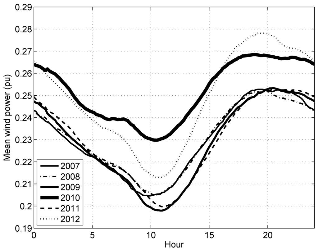
Figure 1.
Daily mean aggregated wind power generation (Spanish power system, 2007–2012) [36].
Figure 1.
Daily mean aggregated wind power generation (Spanish power system, 2007–2012) [36].

Summarizing, wind speed PDF is usually well fit with unimodal models and its main applications are resource assessment and wind farm design. In contrast, wind power PDF is preferred for probabilistic forecast, reserves quantification and stochastic operation in power systems. Furthermore, the ”natural” variability of the wind combined with the power curve and the artificial or imposed variability (curtailments, voltage sags, maintenance, ...) produce important differences with wind speed PDF. When wind power is aggregated, smoothing effect has also taken into account. The novel contribution of this paper is the implementation of PDF model for aggregated wind power production including the effects of the previously described events. This issue is not considered in previous works.
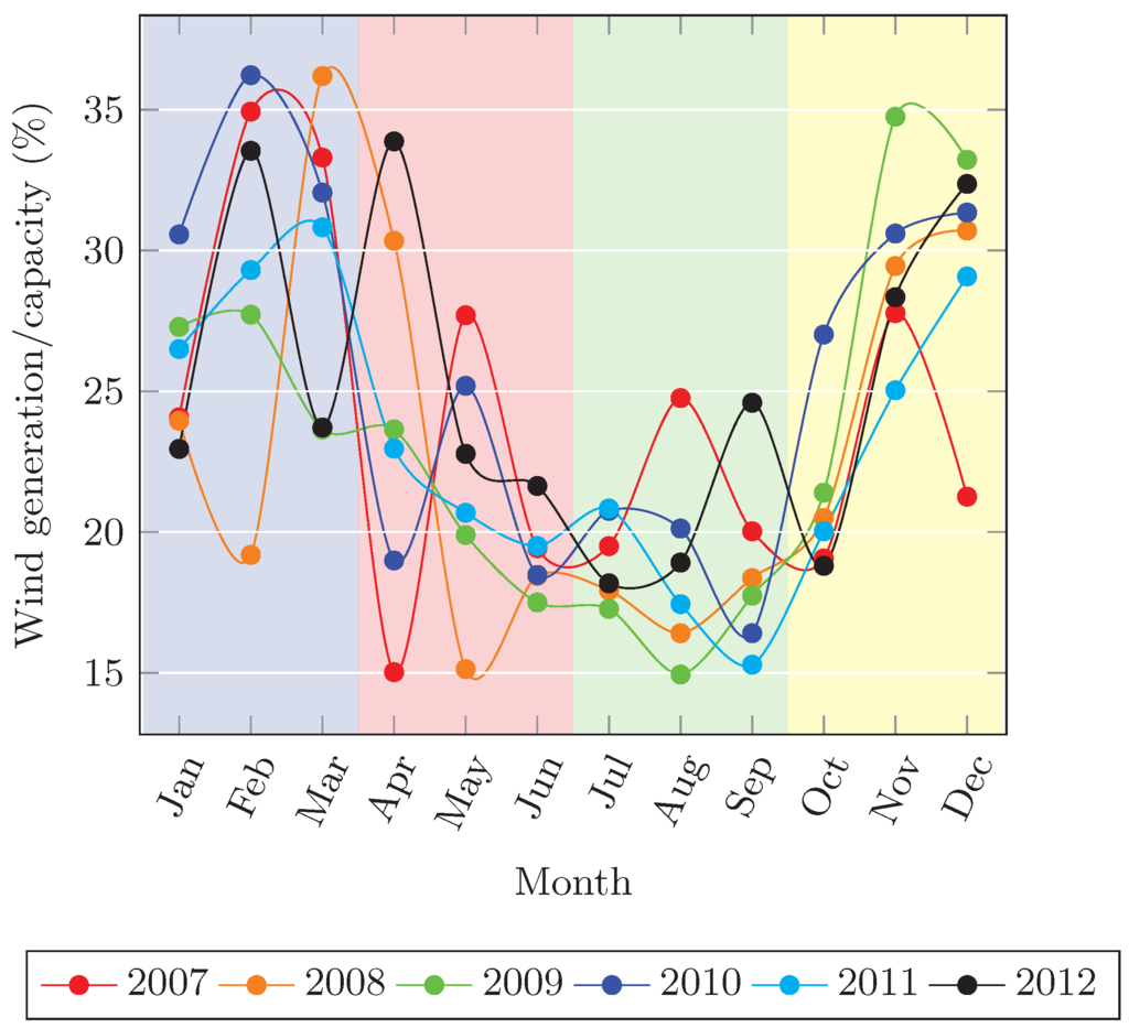
Figure 2.
Aggregated wind power generation (Spanish power system, 2007–2012) [36].
Figure 2.
Aggregated wind power generation (Spanish power system, 2007–2012) [36].

3. The Proposed Model: Weibull Mixture Characterization
In this section, we formulate the Weibull mixture characterization for aggregated wind power production PDFs, describing the model selection criteria as well as the iterative algorithm to estimate their parameters.
3.1. The Mixture Model Formulation
The candidate density function to represent the wind power generation PDF is expressed as:
where c is the number of components; (with ) are the components’ weights required to add 1; is the Weibull density function with parameters , see Equation (1).
A particular and important case is obtained when , in which a single Weibull distribution is fitted to the data. If c is set to 2, the model describes a double-peaked bi-Weibull distribution, whereas if c is set to 3, it describes a tri-Weibull distribution. The weights determine the contribution of each individual Weibull component to the global PDF.
3.2. Estimation and Model Selection
We aim to fit a mixture of Weibull distributions from empirical density functions corresponding to wind power data. To obtain a better fit, a relevant issue is whether to choose a single Weibull distribution, a bi-Weibull, or tri-Weibull distribution. Additional components can also be included, but over-fitting may become an issue. For this reason, parsimonious representations of the data are preferred.
The choice of the number of components in Equation (2) is a model selection problem, and a wide variety of information criteria have been proposed in the literature to compare a finite set of models. The most widely used are the Akaike information criterion (AIC) and the Bayesian information criterion (BIC). A general exposition of information theoretic criteria and model selection can be found in [39].
For a given model, with parameters θ , the AIC is defined as:
where is the maximum likelihood estimator for the model based on the observed data x, is the log-likelihood function evaluated at , and k is the number of parameters involved in the model.
For a given dataset, we can determine the AIC for a single Weibull distribution (), a bi-Weibull (), and a tri-Weibull (). The preferred model is the one that has the lowest AIC [39]. A corrected AIC (AICC) is used for small samples () given by:
where n is the number of observed data.
The (BIC) is defined as:
Given any two proposed models, the model that has the lower value of BIC is preferred. It is generally considered that BIC penalizes the number of parameters in the model more strongly than does AIC, since BIC takes into account the length of the dataset, as seen in the value in Equation (5). Figure 3 shows an example of Weibull estimation where, for the same data source, BIC and AIC suggest a different number of components: BIC selects a single Weibull distribution, and AIC gives a tri-Weibull solution to characterize the empirical density distribution function.
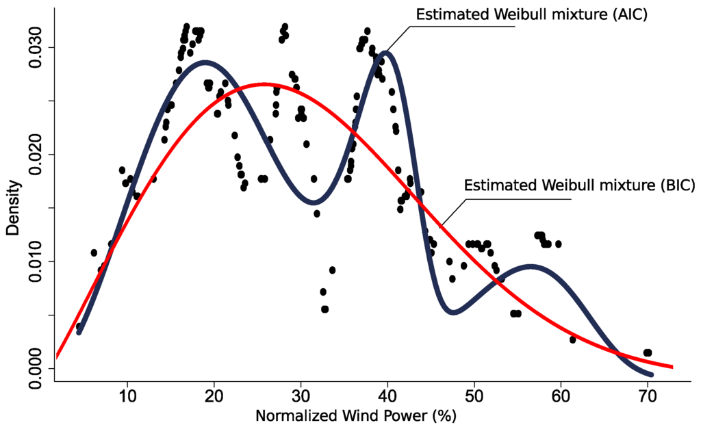
Figure 3.
Example of Weibull mixture estimation for aggregated wind power generation (Bayesian information criterion (BIC) and Akaike information criterion (AIC) approaches).
Figure 3.
Example of Weibull mixture estimation for aggregated wind power generation (Bayesian information criterion (BIC) and Akaike information criterion (AIC) approaches).

To estimate a finite number of Weibull components through both AIC and BIC, an iterative algorithm such as expectation-maximization and its variants are typically used for estimation [40]. In this paper, the rough-enhanced-bayesian finite mixture modeling (REBMIX) algorithm was chosen [41]. It is an iterative algorithm introduced to estimate the component weights and component parameters for finite mixture models [42], particularly tailored to mixtures of Weibull distributions [43]. This algorithm has been implemented in the rebmix package (Version 2.7.1) for R language and environment for statistical computing.
4. Results
4.1. General Overview: Optimal Weibull-Mixture Component Analysis
The Spanish power system is a suitable example of a power system with high wind power penetration, accounting for over 800 wind farms and 20,000 wind turbines. The installed capacity has been increased from 15,071 MW (2007) to 22,784 MW (2012). Real data corresponding to 10-min samples of the Spain’s aggregated wind power generation from 2007 to 2012, including events and operations related to wind power generation, have been used to evaluate the proposed model. The considered 10-min time unit thus provides 6 points per hour. The aggregated data have been normalized by the installed power capacity for each month of the year. Each year is divided into four quarters, from Q1 (January, February and March) to Q4 (October, November and December), according to similarities between monthly wind power generation due to seasonal effects. As a consequence, each bin (year, quarter and hour of the day) includes approximately 540 data points, which is a significant number of samples for a density estimation problem.
With the aim of providing a preliminary example of the proposed methodology, three hours within the fourth quarter (Q4) of year 2010 are analyzed. Figure 4 depicts the empirical density functions and their corresponding Weibull–mixture estimations. Additionally, AIC and BIC values are displayed in Table 1. As can be seen, different numbers of components are selected for each hour, as a consequence of the empirical density profile diversity. In this case, both AIC and BIC lead to the same number of components. These three examples offer an overview of the heterogeneity of aggregated wind power distribution for different hours of an arbitrary day. The results point out the Weibull mixture suitability rather than a unique Weibull probability function to characterize in detail PDFs for certain hours of the daily aggregated wind power generation, particularly when a large-scale aggregated wind power is considered. The number of components can be highly dependent on the high density bins at medium and large wind power values. This is the case study shown in Figure 4b, where two local maximum values can be identified. As described in Section 2, the aggregation of the wind power over large geographic areas and wind power variability can be identified as important causes of the distribution features.

Table 1.
For year 2010, 4th quarter and three different hours of the day, values of the information criteria for the estimated mixture models with c = 1, 2 and 3 components and the estimated weights for the optimum mixture model of aggregated wind power generation.
| Hour | Estimated mixture model | |||
|---|---|---|---|---|
| Criterion | Mono Weibull () | Bi-Weibull () | Tri-Weibull () | |
| 03 | AIC | 4456.16 | 4421.96 | 4404.54 |
| 03 | BIC | 4464.78 | 4443.53 | 4439.05 |
| Optimal estimated weights, c = 3 | - | = 0.44 | = 0.37 | = 0.19 |
| 06 | AIC | 4467.07 | 4409.71 | 4427.02 |
| 06 | BIC | 4475.69 | 4431.28 | 4461.53 |
| Optimal estimated weights, c = 2 | - | 0.63 | 0.37 | |
| 13 | AIC | 4581.82 | 4587.43 | 4615.99 |
| 13 | BIC | 4590.45 | 4609.00 | 4650.50 |
| Optimal estimated weights, c = 1 | - | 1 | - | - |
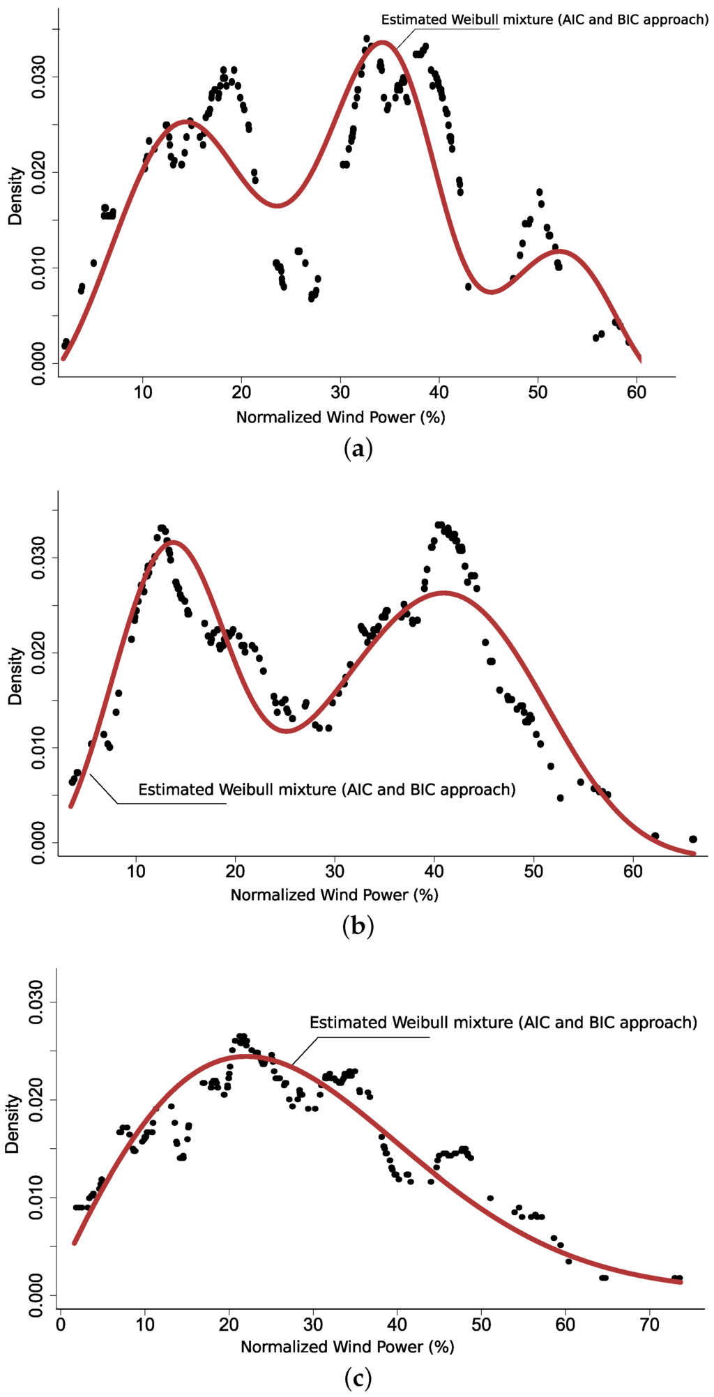
Figure 4.
Empirical density functions and fitted Weibull mixture models of aggregated wind power generation from the observed data at three selected hours of the day for year 2010 and Q4. AIC and BIC approaches lead to the same solution. (a) Year 2010, Q4, hour 03. The fitted distribution is a mixture of three Weibull densities with weights and scale and shape parameters (0.44, 0.37, 0.19), (35.22, 17.47, 52.19), and (6.86, 2.95, 9.73), respectively; (b) year 2010, Q4, hour 06. The fitted distribution is a mixture of two Weibull densities with weights and scale and shape parameters (0.63, 0.37), (41.73, 15.54) and (4.55, 3.18), respectively; and (c) year 2010, Q4, hour 13. The fitted distribution is a mixture of one Weibull density with scale and shape parameters 33.86 and 1.95, respectively.

4.2. Discussion of Seasonal Weibull–Parameters
An extension of the previous analysis is based on discussing the hourly pattern evolution of the estimated parameters (shape, scale, and weights), comparing the AIC and BIC model selection. Therefore, and as an example of a quarter for a given year, hourly wind power distribution for the entire fourth-quarter (Q4) of the year 2010 is discussed. Figure 5 shows the estimated weights, scale, and shape parameters for AIC and BIC approaches to estimate the optimal number of components. The number of Weibull mixture components is associated with the number of relative maximum values (peaks in the distribution), which are identified based on the empirical density function profiles. In addition, the scale parameter gives information about the position of each Weibull component, being the shape parameter associated with the slope of the peaks.
Regarding the shape parameter, it is smaller and then closer to 1 when a dominating component —in terms of weight in the mixture—can be identified. This fact is particularly relevant for the one-component cases. This smaller value of the shape parameter is associated with a positive skew distribution (probability mass closer to 0), which can be observed when the data can be fitted more accurately with a single-Weibull, see Figure 4c. When more components are estimated, the mixture itself allows for more flexibility of the skewness characteristic of the resulting distribution and each component usually present a larger shape parameter (almost symmetric distribution).
Considering first the AIC-based solution, see Figure 5a,b, it is pointed out that the density bins are fitted with tri-Weibull mixtures during the night time hours (from Hour 0 to Hour 5). Furthermore, Figure 5a,b shows that the winter-spring demand peak hour, around 8 p.m., is also fitted with a tri–Weibull mixture. This is in line with the wind power curtailment influence on the overall distribution shape, since these hours correspond to relatively high levels of wind power curtailment and have noticeably different distribution shapes.
The weight of the third component is not available for other periods of the day. Consequently, the wind power generation distribution is characterized through a single Weibull density function. The scale parameter is increasing during the afternoon and evening time hours, giving rise to a second and third well–separated Weibull-component. For the rest of the hours, this parameter remains in similar values for the main component of the mixture, independently from the other Weibull component. For hours with medium power demand, bi-Weibull components are suggested to characterize the aggregated wind power generation histogram.
As an example of the imposed varibility influence in the PDF, the hours with highly variable power and curtailments, i.e., those times that usually contain large and sudden wind generation changes, normally present large additional peaks in their probability functions and are thus better characterized by bi- and tri-Weibull mixtures. The number of additional components can be then associated with the characteristics and the quantity of the curtailment periods. For the rest of the hours, no wind curtailments or wind curtailment actions that are applied in a less drastic manner are usually applied and the generated wind power distribution is properly modeled by a single Weibull density.
When BIC is selected as model selection criterion, see Figure 5c,d, more conservative results in terms of the number of components are obtained. This is to be expected due to the BIC penalizes significantly the number of components, as detailed in Section 3. Nevertheless, in hours with high wind power curtailments, the distribution profiles are more accurately characterized with three– Weibull components, presenting scale and shape parameters similar to the previous approach. This result confirms the relevance and necessity of a mixture of distributions to characterize and estimate aggregated wind power generation density function for real power system data. Spite a more conservative criterion is used, the shape of the density function and the existence of peaks calls for several Weibull components.
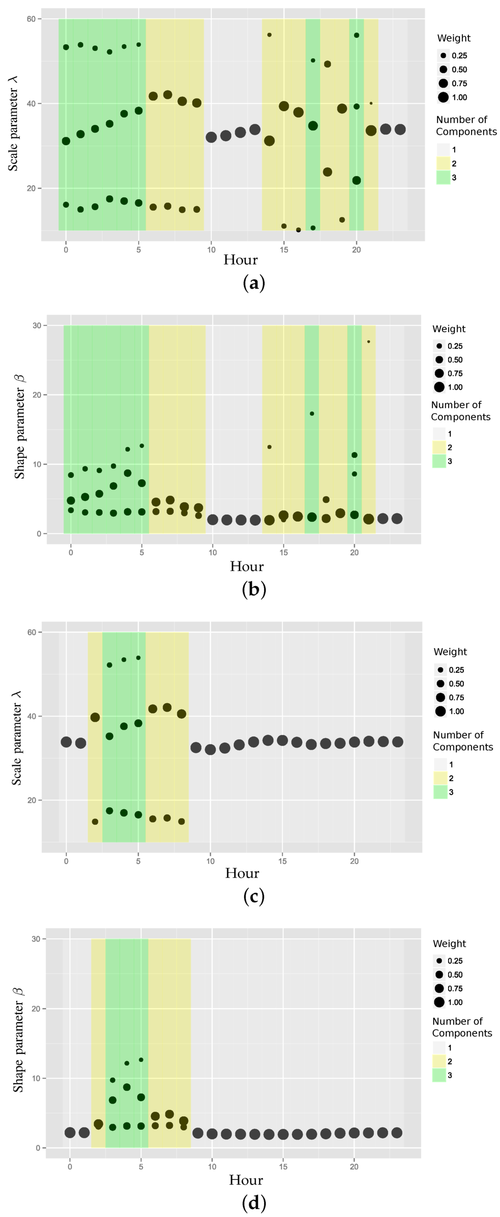
Figure 5.
Number of components (according to rough-enhanced-bayesian finite mixture modeling (REBMIX) algorithm), estimated weights, scale and shape parameters for Q4 of year 2010 using wind power generation data. The size of the plotted points is proportional to the estimated weights of the corresponding fitted mixture of Weibull distribution. (a) Scale parameter λ. AIC approach; (b) shape parameter β. AIC approach; (c) scale parameter λ. BIC approach; and (d) shape parameter β. BIC approach.

4.3. Comparison of Optimal Number of Components in the Fitted Weibull-Mixture
This Section is focused on estimating the number of optimal components for the Weibull mixture, considering both AIC and BIC approaches, for all years and quarters. Subsequently, all years from 2007 to 2012 are considered and the hourly pattern of the selected number of components for the fitted Weibull–mixture model is discussed for each quarter. Both AIC and BIC are thus considered and the corresponding results are summarized in Figure 6, where a color code is proposed to identify the optimal number of Weibull-mixture components for each hour of the day. From this analysis, Weibull mixtures with two and three components are relatively common, as discussed in Section 4.2. The number of Weibull components depends on the analyzed year and quarter, as well as on the season of the year. As shown in the previous section, curtailment actions clearly affect the aggregated wind power generation evolution and consequently the corresponding optimal Weibull-mixture, though they are not the only parameters with influence on the aggregated wind power PDF multi-modality. For the context of the Spanish power system, until 2009, larger wind power curtailments were applied due to important grid limitations at the distribution level. Since the end of 2009, wind power curtailments have been programmed in real time based on the scheduled mix of generation and according to the ”Non-integrable wind power excess” as defined by the Spanish transmission system operations within the operational procedure 3.7 [44]. Curtailments typically start between 9 p.m. and 1 a.m. and finish between 5 a.m. and 8 a.m., depending on the season and the operating conditions. This fact contributes strongly to the need for additional Weibull components aiming to characterize properly the distributions during high wind periods, especially in spring and autumn. Table 2 and Table 3 summarize the relative frequencies for each year of the optimal number of Weibull components according to BIC and AIC, respectively.
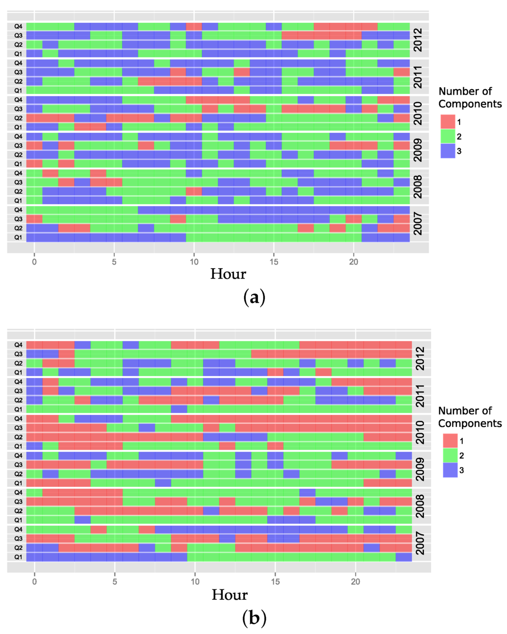
Figure 6.
AIC and BIC approaches: optimal number of components for the Weibull mixture model according to the hour of the day for Q1 through Q4 for the years 2007–2012 using wind power generation data. (a) AIC approach; and (b) BIC approach.
Figure 6.
AIC and BIC approaches: optimal number of components for the Weibull mixture model according to the hour of the day for Q1 through Q4 for the years 2007–2012 using wind power generation data. (a) AIC approach; and (b) BIC approach.

Table 2.
Relative frequencies of the optimal number of Weibull components (AIC approach) using aggregated wind power generation data.
| Weibull components | Percentage of components by years | Total | |||||
|---|---|---|---|---|---|---|---|
| 2007 | 2008 | 2009 | 2010 | 2011 | 2012 | ||
| 1 | 10% | 6% | 9% | 26% | 7% | 10% | 12% |
| 2 | 46% | 55% | 43% | 45% | 39% | 43% | 45% |
| 3 | 44% | 39% | 48% | 29% | 54% | 47% | 43% |
Table 3.
Relative frequencies of the optimal number of Weibull components (BIC approach) using aggregated wind power generation data.
| Weibull components | Percentage of components by years | Total | |||||
|---|---|---|---|---|---|---|---|
| 2007 | 2008 | 2009 | 2010 | 2011 | 2012 | ||
| 1 | 34% | 32% | 23% | 56% | 27% | 29% | 34% |
| 2 | 32% | 57% | 50% | 34% | 44% | 49% | 44% |
| 3 | 33% | 10% | 27% | 9% | 29% | 22% | 22% |
As previously discussed, the BIC tends to favor a smaller number of Weibull components compared to AIC. Nevertheless, when using the BIC approach, around 66% of the aggregated hourly wind power generation distributions should be characterized by using more than one Weibull component. To complete this analysis, a comparison between the number of Weibull components selected by AIC and BIC is illustrated in Figure 7. In most cases, there is no difference between the optimal number of components when comparing between the criteria. In fact, around 70% of the estimations give the same number of components by both approaches. Therefore, the proposed solution provide a suitable and accurate estimation for aggregated wind power PDF by using a mixture of a simple and reliable distribution: Weibull. The use of this alternative approach with historical data provides a tool based on probabilistic methodology for the applications previously described: reserve estimation, forecast, etc. In addition, this solution can be also applied on other aggregated wind power dataset, obtaining more accurate mixtures to fit the corresponding PDF. The percentage of each mixture would vary according to the wind speed variability, curtailments or smoothing effects due to the aggregated power output from geographically dispersed wind farms.
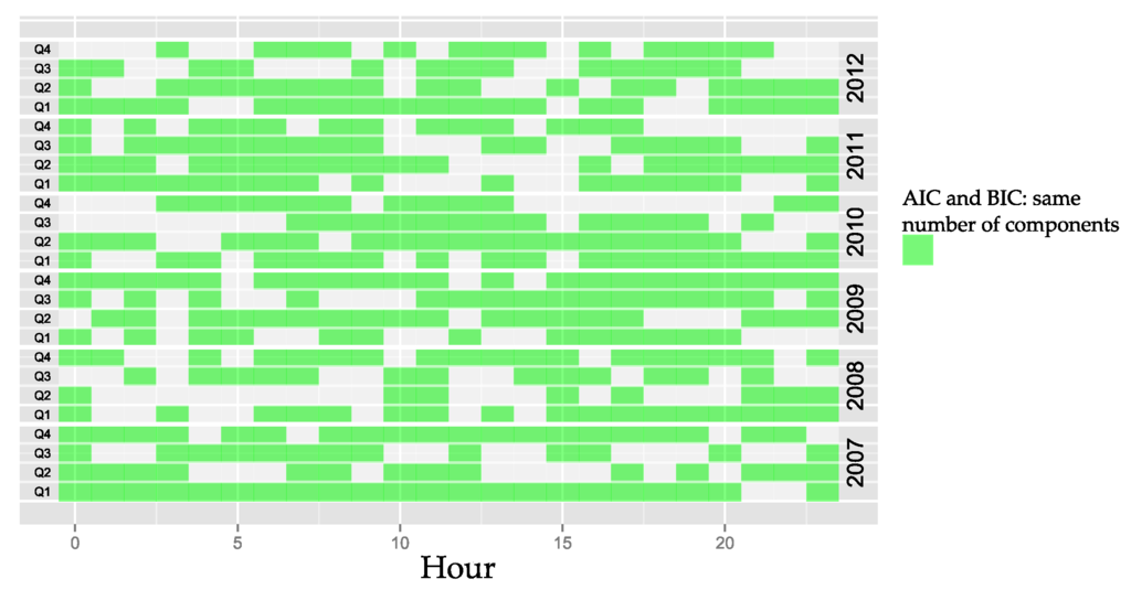
Figure 7.
Weibull mixture model divided into quarters from aggregated wind power generation data (2007–2012). Hours with similar optimal number of components for AIC and BIC.
Figure 7.
Weibull mixture model divided into quarters from aggregated wind power generation data (2007–2012). Hours with similar optimal number of components for AIC and BIC.

5. Conclusions
This paper proposed and evaluated a Weibull mixture as a solution to estimate PDFs for aggregated wind power generation. The smoothing effects of geographical dispersion, wind power aggregation and operational actions carried out by the TSO affect the estimation of the PDFs for different hours of the day, and then, different Weibull mixture components should be estimated. To determine this optimal number of Weibull components, two different well-known information-based criteria have been proposed: the BIC and AIC approaches. A comparison between both criteria is carried out for different hours of the day and seasons. The estimated Weibull mixtures by using both criteria mostly yields similar results, providing the same number of components for around 70% of the hours and quarters analyzed. Consequently, the selection of AIC or BIC is not critical in this case.
Specific Weibull mixture parameters —estimated weight, scale, and shape parameters— are also discussed in detail for different periods and operational considerations. Aggregated wind power production along several years from the Spanish power system is used to provide extensive analysis of the proposed Weibull–mixture approach. The results show that over 66% of the aggregated hourly wind power generation PDF require more than one–Weibull component to be accurately characterized. More specifically, 44% are modeled by bi-Weibull distributions and 22% corresponds to tri-Weibull distributions. This is a clear contrast with the single Weibull component, which is typically proposed for the characterization of wind speed distributions and, according to the results, it should be not extended to the aggregated wind power generation characterization.
Acknowledgments
This work was supported by ”Ministerio de Economía y Competitividad” and the European Union —ENE2012-34603—, Fulbright/Spanish Ministry of Education Visiting Scholar —PRX14/00694—, and by the U.S. Department of Energy under Contract No. DE-AC36-08-GO28308 with the National Renewable Energy Laboratory.
Author Contributions
Emilio Gómez-Lázaro, Sergio Martín-Martínez and Angel Molina-García conceived and designed the simulations and the paper scope; María C. Bueso and Mathieu Kessler performed the simulations; Sergio Martín-Martínez, Angel Molina-García, Jie Zhang, and Bri-Mathias Hodge analyzed the data; All the authors wrote sections of the paper.
Conflicts of Interest
The authors declare no conflict of interest.
References
- Bollen, M.H.; Hassan, F. Integration of Distributed Generation in the Power System; John Wiley & Sons: Hoboken, NJ, USA, 2011; Volume 80. [Google Scholar]
- Estanqueiro, A.; Rygg-Ardal, A.; O’Dwyer, C.; Flynn, D.; Huertas-Hernando, D.; Lew, D.; Gómez-Lázaro, E.; Ela, E.; Revuelta, J.; Kiviluoma, J.; et al. Energy Storage for Wind Integration: Hydropower and Other Contributions. In Proceedings of the IEEE Power and Energy Society General Meeting, San Diego, CA, USA, 22–26 July 2012; pp. 1–6.
- Hodge, B.M.; Holttinen, H.; Sillanpä, S.; Gómez-Lázaro, E.; Scharff, R.; Larsen, X.G.; Giebel, G.; Flynn, D.; Lew, D.; Milligan, M. Wind Power Forecasting Error Distributions: An International Comparison. In Proceedings of the 11th Annual International Workshop on Large-Scale Integration of Wind Power into Power Systems as well as on Transmission Networks for Offshore Wind Power Plants Conference, Lisbon, Portugal, 13–15 November 2012; pp. 1–7.
- Ela, E.; O’Malley, M. Studying the Variability and Uncertainty Impacts of Variable Generation at Multiple Timescales. IEEE Trans. Power Syst. 2012, 27, 1324–1333. [Google Scholar] [CrossRef]
- Milligan, M.; Donohoo, P.; Lew, D.; Ela, E.; Kirby, B.; Holttinen, H.; Lannoye, E.; Flynn, D.; O’Malley, M.; Miller, N.; et al. Operating Reserves and Wind Power Integration: An International Comparison. In Proceedings of the 9th Annual International Workshop on Large-Scale Integration of Wind Power into Power Systems as well as on Transmission Networks for Offshore Wind Power Plants Conference, Québec, QC, Canada, 18–19 October 2010; pp. 383–398.
- Maisonneuve, N.; Gross, G. A Production Simulation Tool for Systems With Integrated Wind Energy Resources. IEEE Trans. Power Syst. 2011, 26, 2285–2292. [Google Scholar] [CrossRef]
- Wang, P.; Gao, Z.; Bertling, L. Operational Adequacy Studies of Power Systems with Wind Farms and Energy Storages. IEEE Trans. Power Syst. 2012, 27, 2377–2384. [Google Scholar] [CrossRef]
- Aigner, T.; Jaehnert, S.; Doorman, G.; Gjengedal, T. The effect of large-scale wind power on system balancing in Northern Europe. IEEE Trans. Sustain. Energy 2012, 3, 751–759. [Google Scholar] [CrossRef]
- Chen, N.; Qian, Z.; Nabney, I.; Meng, X. Wind power forecasts using Gaussian processes and numerical weather prediction. IEEE Trans. Power Syst. 2014, 29, 656–665. [Google Scholar] [CrossRef]
- Haque, A.; Nehrir, M.; Mandal, P. A Hybrid Intelligent Model for Deterministic and Quantile Regression Approach for Probabilistic Wind Power Forecasting. IEEE Trans. Power Syst. 2014, 29, 1663–1672. [Google Scholar] [CrossRef]
- Zhang, Z.S.; Sun, Y.Z.; Gao, D.; Lin, J.; Cheng, L. A Versatile Probability Distribution Model for Wind Power Forecast Errors and Its Application in Economic Dispatch. IEEE Trans. Power Syst. 2013, 28, 3114–3125. [Google Scholar] [CrossRef]
- Qin, Z.; Li, W.; Xiong, X. Generation System Reliability Evaluation Incorporating Correlations of Wind Speeds with Different Distributions. IEEE Trans. Power Syst. 2013, 28, 551–558. [Google Scholar] [CrossRef]
- Kollu, R.; Rayapudi, S.R.; Narasimham, S.; Pakkurthi, K.M. Mixture probability distribution functions to model wind speed distributions. Int. J. Energy Environ. Eng. 2012, 3, 2–10. [Google Scholar] [CrossRef]
- Hennessey, J.P., Jr. Some aspects of wind power statistics. J. Appl. Meteorol. 1977, 16, 119–128. [Google Scholar] [CrossRef]
- Justus, C.; Hargraves, W.; Mikhail, A.; Graber, D. Methods for estimating wind speed frequency distributions. J. Appl. Meteorol. 1978, 17, 350–353. [Google Scholar] [CrossRef]
- Conradsen, K.; Nielsen, L.; Prahm, L. Review of Weibull statistics for estimation of wind speed distributions. J. Clim. Appl. Meteorol. 1984, 23, 1173–1183. [Google Scholar] [CrossRef]
- Lun, I.Y.; Lam, J.C. A study of Weibull parameters using long-term wind observations. Renew. Energy 2000, 20, 145–153. [Google Scholar] [CrossRef]
- Seguro, J.; Lambert, T. Modern estimation of the parameters of the Weibull wind speed distribution for wind energy analysis. J. Wind Eng. Ind. Aerodyn. 2000, 85, 75–84. [Google Scholar] [CrossRef]
- Wind Turbines Part 12-1: Power Performance Measurements of Electricity Producing Wind Turbines; IEC 61400-12-1:2005; International Electrotechnical Commission: Geneva, Switzerland, 2005.
- Burton, T.; Jenkins, N.; Sharpe, D.; Bossanyi, E. Wind Energy Handbook; John Wiley & Sons: Chichester, UK, 2011. [Google Scholar]
- Gualtieri, G.; Secci, S. Extrapolating wind speed time series vs. Weibull distribution to assess wind resource to the turbine hub height: A case study on coastal location in Southern Italy. Renew. Energy 2014, 62, 164–176. [Google Scholar] [CrossRef]
- Ohunakin, O.S. Assessment of wind energy resources for electricity generation using WECS in North-Central region, Nigeria. Renew. Sustain. Energy Rev. 2011, 15, 1968–1976. [Google Scholar] [CrossRef]
- Carta, J.; Ramirez, P. Analysis of two-component mixture Weibull statistics for estimation of wind speed distributions. Renew. Energy 2007, 32, 518–531. [Google Scholar] [CrossRef]
- Akpinar, S.; Akpinar, E.K. Estimation of wind energy potential using finite mixture distribution models. Energy Convers. Manag. 2009, 50, 877–884. [Google Scholar] [CrossRef]
- Akdağ, S.; Bagiorgas, H.; Mihalakakou, G. Use of two-component Weibull mixtures in the analysis of wind speed in the Eastern Mediterranean. Appl. Energy 2010, 87, 2566–2573. [Google Scholar] [CrossRef]
- Jaramillo, O.; Borja, M. Wind speed analysis in La Ventosa, Mexico: A bimodal probability distribution case. Renew. Energy 2004, 29, 1613–1630. [Google Scholar] [CrossRef]
- Chang, T.P. Performance comparison of six numerical methods in estimating Weibull parameters for wind energy application. Appl. Energy 2011, 88, 272–282. [Google Scholar] [CrossRef]
- Ramírez, P.; Carta, J.A. Influence of the data sampling interval in the estimation of the parameters of the Weibull wind speed probability density distribution: A case study. Energy Convers. Manag. 2005, 46, 2419–2438. [Google Scholar] [CrossRef]
- Chang, T.P. Estimation of wind energy potential using different probability density functions. Appl. Energy 2011, 88, 1848–1856. [Google Scholar] [CrossRef]
- Carta, J.A.; Ramirez, P.; Velazquez, S. A review of wind speed probability distributions used in wind energy analysis: Case studies in the Canary Islands. Renew. Sustain. Energy Rev. 2009, 13, 933–955. [Google Scholar] [CrossRef]
- Chang, T.P. Wind Speed and Power Density Analyses Based on Mixture Weibull and Maximum Entropy Distributions. Int. J. Appl. Sci. Eng. 2010, 8, 39–46. [Google Scholar]
- Carta, J.A.; Ramírez, P.; Velázquez, S. Influence of the level of fit of a density probability function to wind-speed data on the WECS mean power output estimation. Energy Convers. Manag. 2008, 49, 2647–2655. [Google Scholar] [CrossRef]
- Ackermann, T. Wind Power in Power Systems; Wiley Online Library: Chichester, UK, 2005; Volume 140. [Google Scholar]
- Holttinen, H.; Meibom, P.; Orths, A.; Lange, B.; O’Malley, M.; Tande, J.O.; Estanqueiro, A.; Gomez, E.; Söder, L.; Strbac, G.; et al. Impacts of large amounts of wind power on design and operation of power systems, results of IEA collaboration. Wind Energy 2011, 14, 179–192. [Google Scholar] [CrossRef]
- Coughlin, K. Analysis of Wind Power and Load Data at Multiple Time Scales; Lawrence Berkeley National Laboratory: Berkeley, CA, USA, 2011. [Google Scholar]
- Asociación Empresarial Eólica (AEE) (Spanish Wind Energy Association), 2015. Available online: http://www.aeeolica.org/ (accessed on 29 January 2016).
- Martín-Martínez, S.; Gómez-Lázaro, E.; Molina-García, A.; Vigueras-Rodriguez, A.; Milligan, M.; Muljadi, E. Participation of wind power plants in the Spanish power system during events. In Proceedings of the IEEE Power and Energy Society General Meeting, San Diego, CA, USA, 22–26 July 2012; pp. 1–8.
- Wan, Y. Long-Term Wind Power Variability; National Renewable Energy Laboratory: Golden, CO, USA, 2012. [Google Scholar]
- Burnham, K.P.; Anderson, D.R. Model Selection and Multimodel Inference: A Practical Information-Theoretic Approach, 2nd ed.; Springer: New York, NY, USA, 2002; pp. 1–488. [Google Scholar]
- McLachlan, G.J.; Peel, D. Finite Mixture Models; Wiley Series in Probability and Statistics: New York, NY, USA, 2000. [Google Scholar]
- Volk, M.; Nagode, M.; Fajdiga, M. Finite Mixture Estimation Algorithm for Arbitrary Function Approximation. J. Mech. Eng. 2012, 58, 115–124. [Google Scholar] [CrossRef]
- Nagode, M.; Fajdiga, M. The REBMIX Algorithm for the Univariate Finite Mixture Estimation. Commun. Stat. Theory Methods 2011, 40, 876–892. [Google Scholar] [CrossRef]
- Nagode, M. Finite mixture modeling via rebmix. J. Algorithms Optim. 2015, 3, 14–28. [Google Scholar] [CrossRef]
- Schedule Generation from Unmanageable Renewable Energy Sources (P.O. 3.7); Spanish Transmission and System Operator (REE): Madrid, Spain, 2009.
© 2016 by the authors; licensee MDPI, Basel, Switzerland. This article is an open access article distributed under the terms and conditions of the Creative Commons by Attribution (CC-BY) license (http://creativecommons.org/licenses/by/4.0/).