
Aerodynamic and Structural Integrated Optimization Design of Horizontal-Axis Wind Turbine Blades


Abstract
:1. Introduction
2. Modeling of the Blade
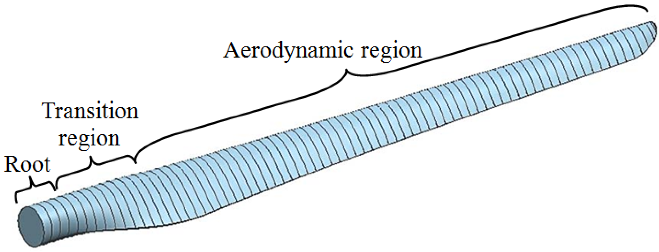
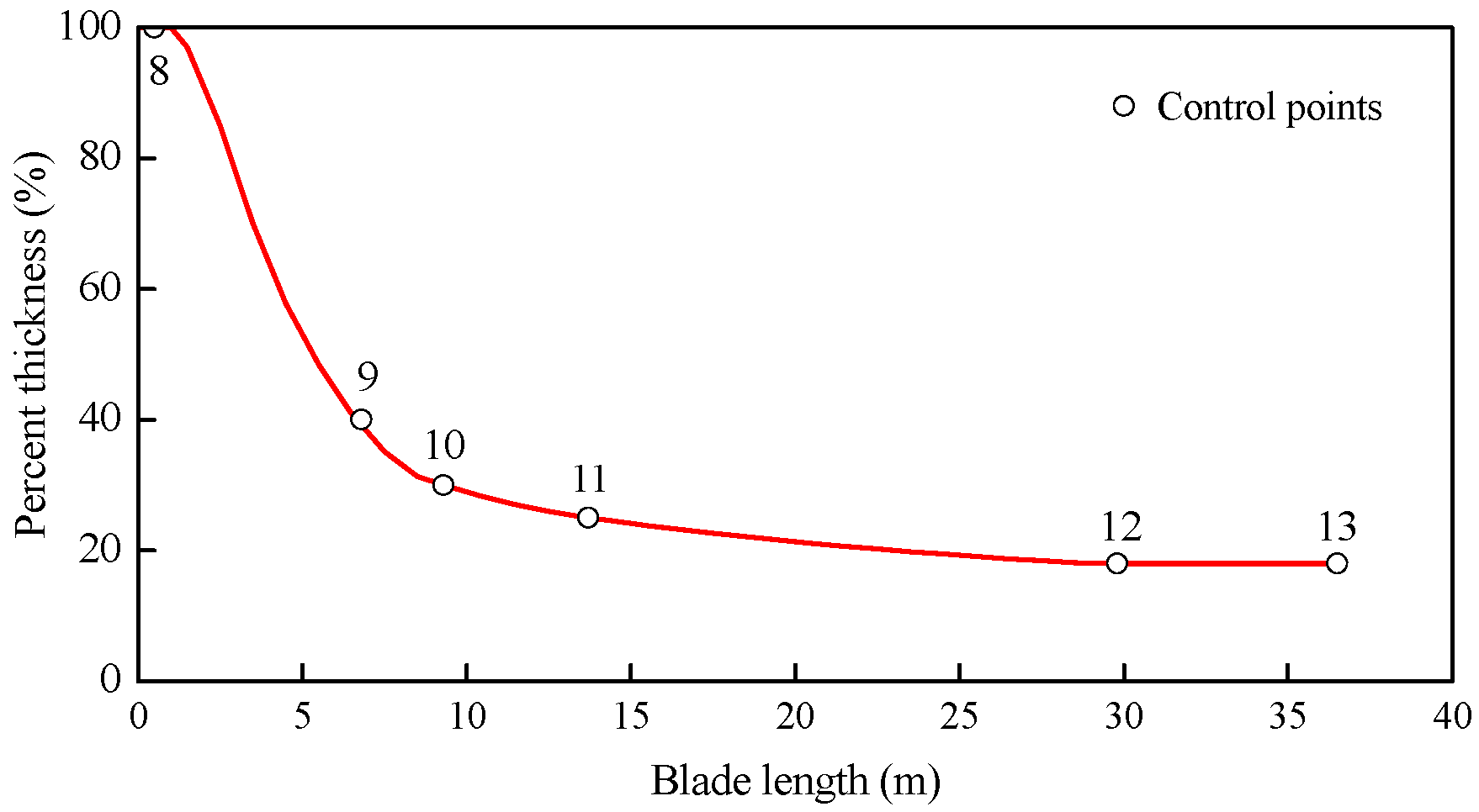
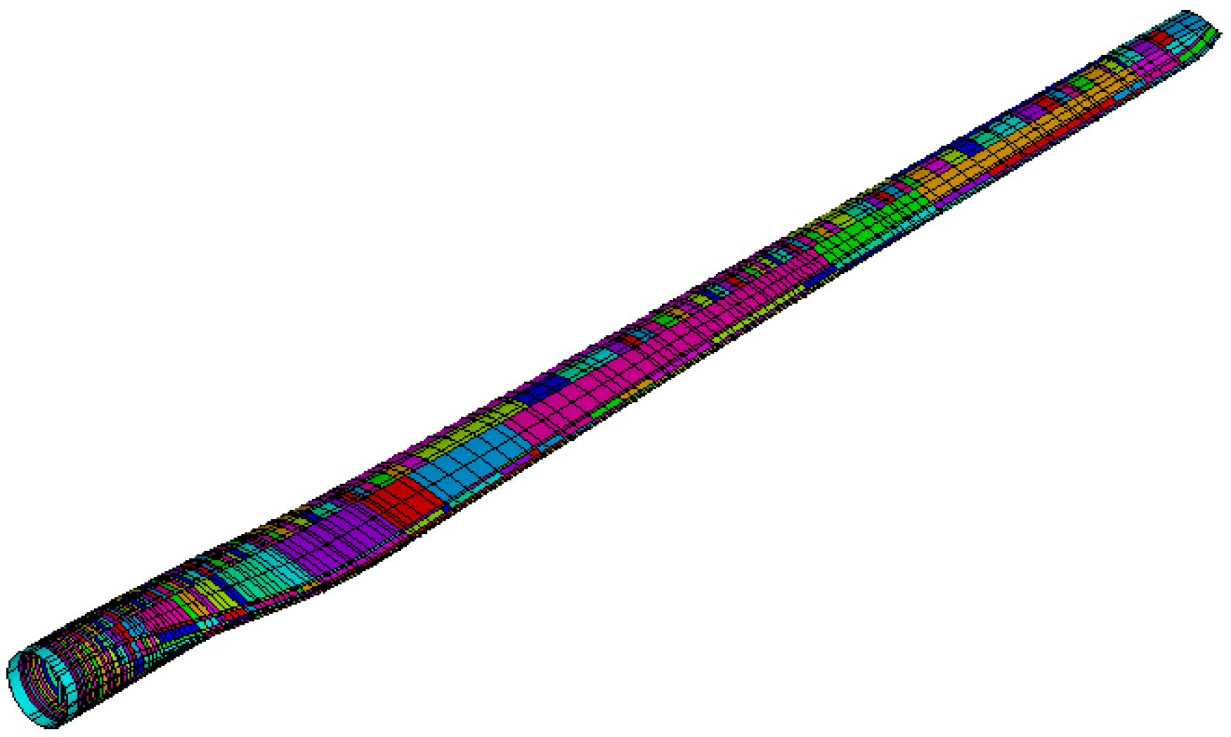
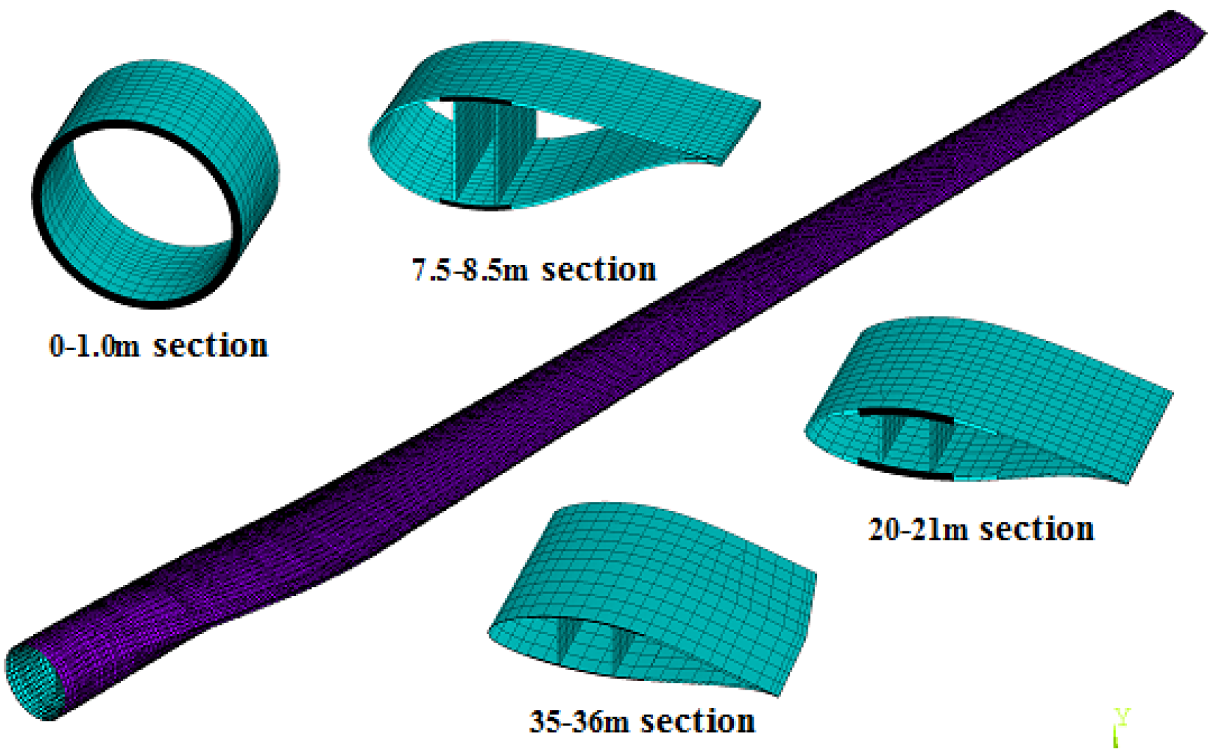
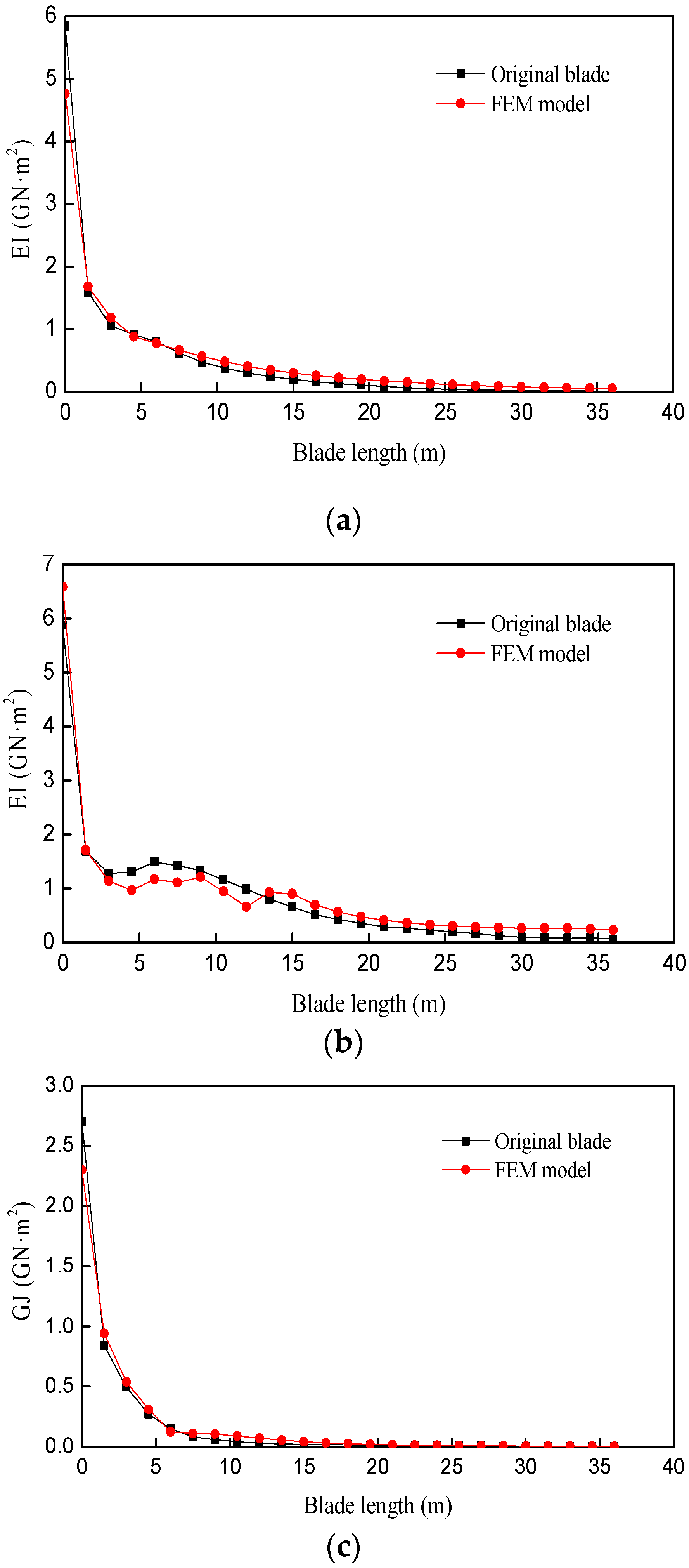
2.1. Finite Element Method (FEM) Model of the Blade


| Location (m) | Airfoil | Chord (m) | Twist (°) | Percent Thickness (%) |
|---|---|---|---|---|
| 0 | Circle | 1.88 | 10.00 | 100 |
| 1.0 | Circle | 1.88 | 10.00 | 100 |
| 6.8 | DU400EU | 3.02 | 10.00 | 40 |
| 9.3 | DU300EU | 2.98 | 7.30 | 30 |
| 13.7 | DU91_W2_250 | 2.51 | 4.35 | 25 |
| 29.8 | NACA_64_618 | 1.68 | −0.33 | 18 |
| 36.5 | NACA_64_618 | 1.21 | −1.13 | 18 |

| Material | E1 (GPa) | E2 (GPa) | G12 (GPa) | v12 | ρ (kg/m3) | Thickness (mm) |
|---|---|---|---|---|---|---|
| UD-1200-xxx | 42.2 | 12.5 | 3.5 | 0.24 | 1910 | 0.873 |
| 2AX-1200-0660 | 11.5 | 11.5 | 11.8 | 0.61 | 1909 | 0.878 |
| 3AX-1200-6330 | 26.9 | 13.4 | 7.5 | 0.47 | 1910 | 0.906 |
| 3AX9060-1200-0336 | 31.8 | 11.4 | 6.5 | 0.49 | 1910 | 0.906 |
| Balsa | 3.5 | 0.8 | 0.16 | 0.39 | 151 | 25.4 |
| PVC | 0.05 | 0.05 | 0.02 | 0.09 | 60 | 10/15/20/25 |


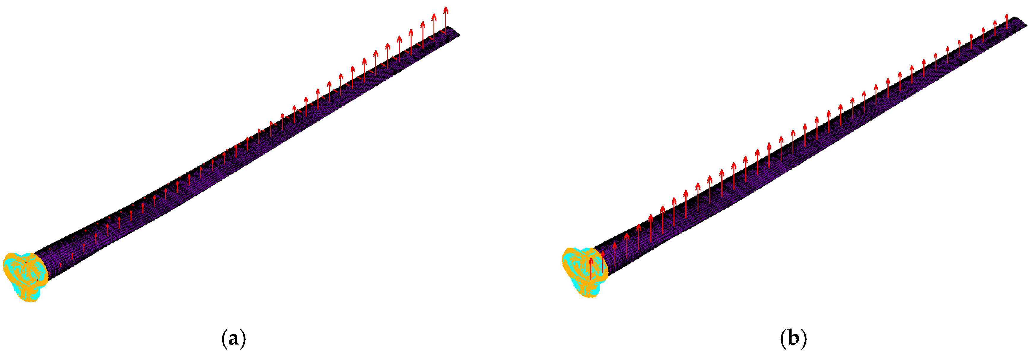
2.2. Aerodynamic Loads of the Blade

3. Formulation of the Optimization Problem
3.1. The Objective Functions
3.2. Design Variables


3.3. Constraint Conditions
| Parameter | Lower Bound | Upper Bound | Unit |
|---|---|---|---|
| x1-x5 | 1.0 | 3.3 | m |
| x6-x10 | −2.0 | 12.0 | ° |
| x11-x14 | 6.0 | 30.0 | m |
| x15 | 10 | 25 | rpm |
| x16 | 28 | 38 | - |
| x17 | 28 | 48 | - |
| x18 | 33 | 58 | - |
| x19 | 35 | 65 | - |
| x20 | 33 | 55 | - |
| x21 | 28 | 45 | - |
| x22 | 28 | 40 | - |
| x23 | 7.0 | 9.0 | m |
| x24 | 10.0 | 13.0 | m |
| x25 | 16.0 | 19.0 | m |
| x26 | 20.5 | 22.0 | m |
| x27 | 0.13 | 0.25 | m |
| x28 | 0.50 | 0.70 | m |
| εmax | - | 0.005 | - |
| dmax | - | 5.5 | m |
| λ1 | 1.2 | - | - |
| Fblade-1 | ≤3Frotor − 0.3 or ≥3Frotor + 0.3 | Hz | |
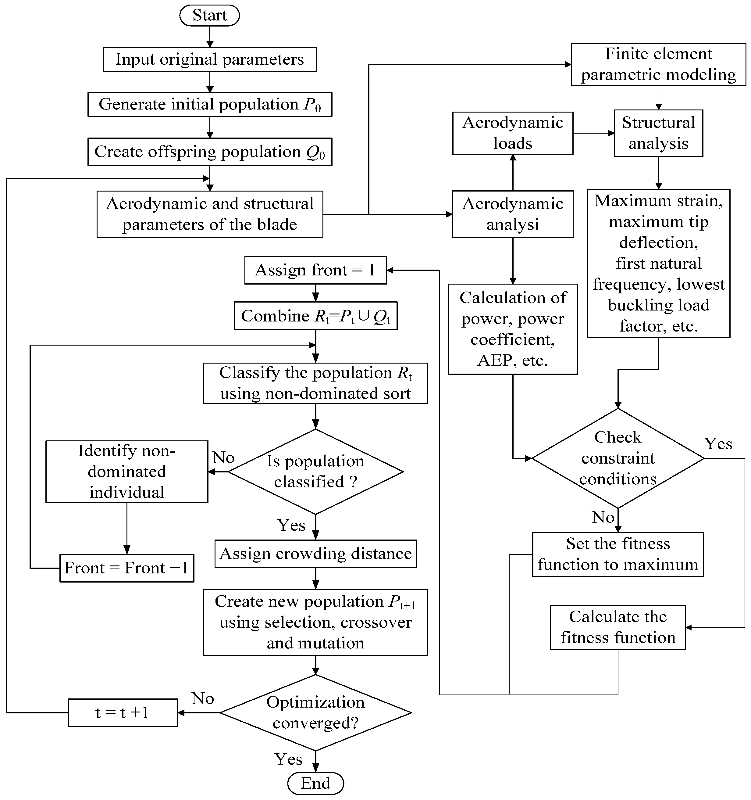
4. The Integrated Optimization Design Procedure

5. Optimization Application and Results
| Parameter | Value | Unit |
|---|---|---|
| Rotor diameter | 77 | m |
| Number of blades | 3 | - |
| Hub diameter | 3 | m |
| Hub height | 75 | m |
| Rated wind speed | 12 | m/s |
| Rated rotational speed | 19 | rpm |
| Rated power | 1500 | kW |
| Cut-in wind speed | 4 | m/s |
| Cut-out wind speed | 25 | m/s |
| Air density | 1.225 | kg/m3 |
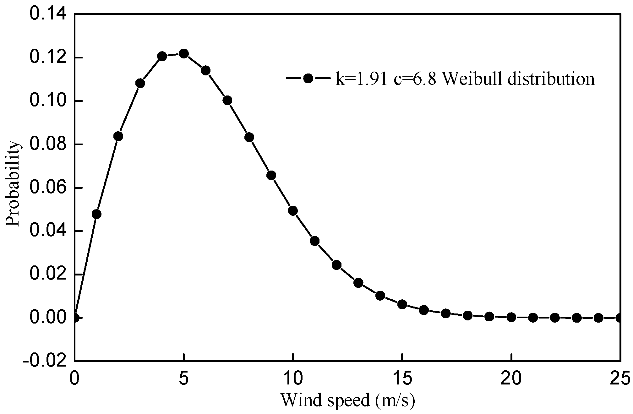
| Weibull form factor k | 1.91 | - |
| Weibull scaling factor A | 6.8 | m/s |
| Number of individuals | 40 | - |
| Number of iterations | 30 | - |
| Probability of crossover | 0.8 | - |
| Probability of mutation | 0.05 | - |

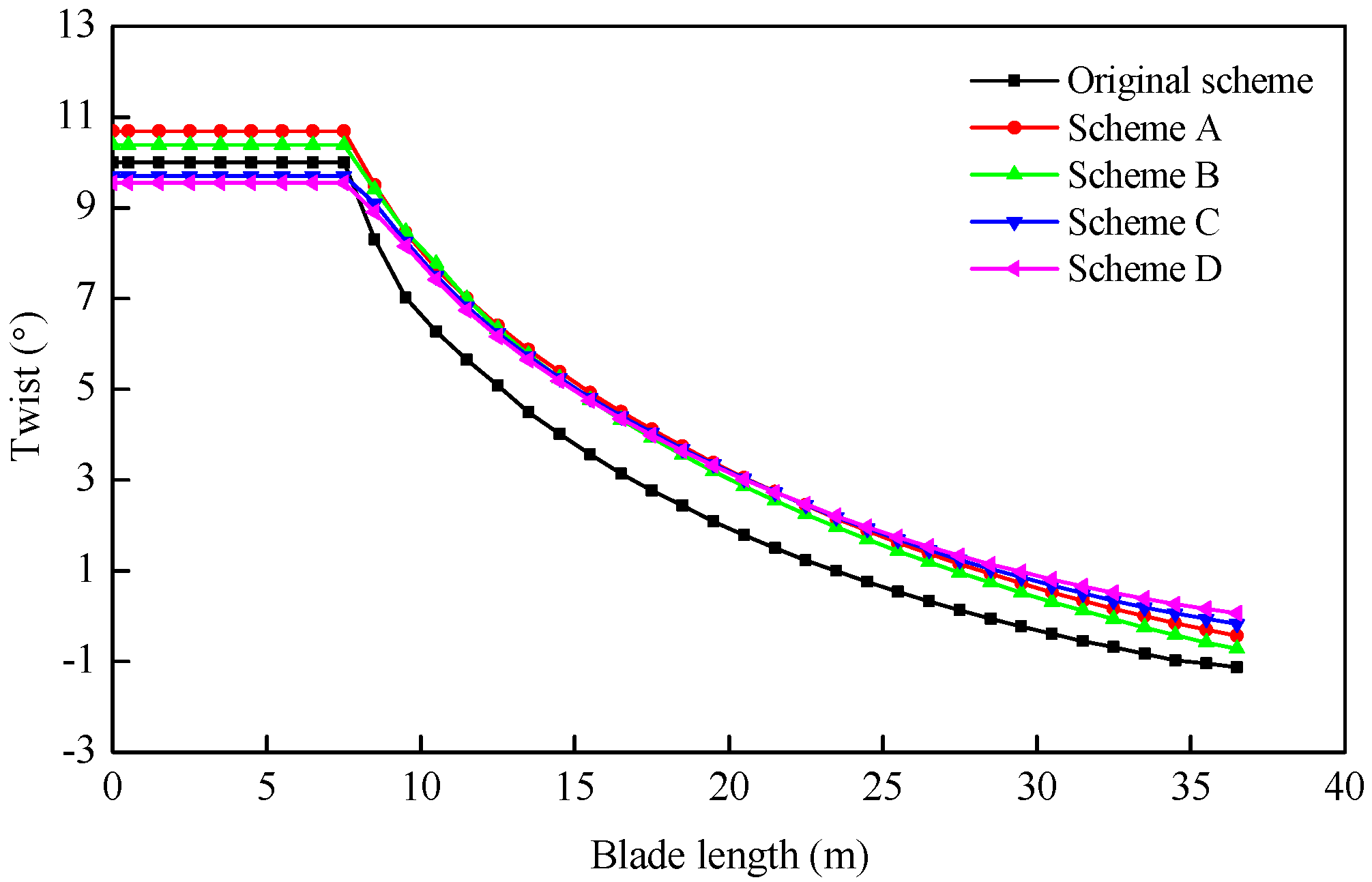
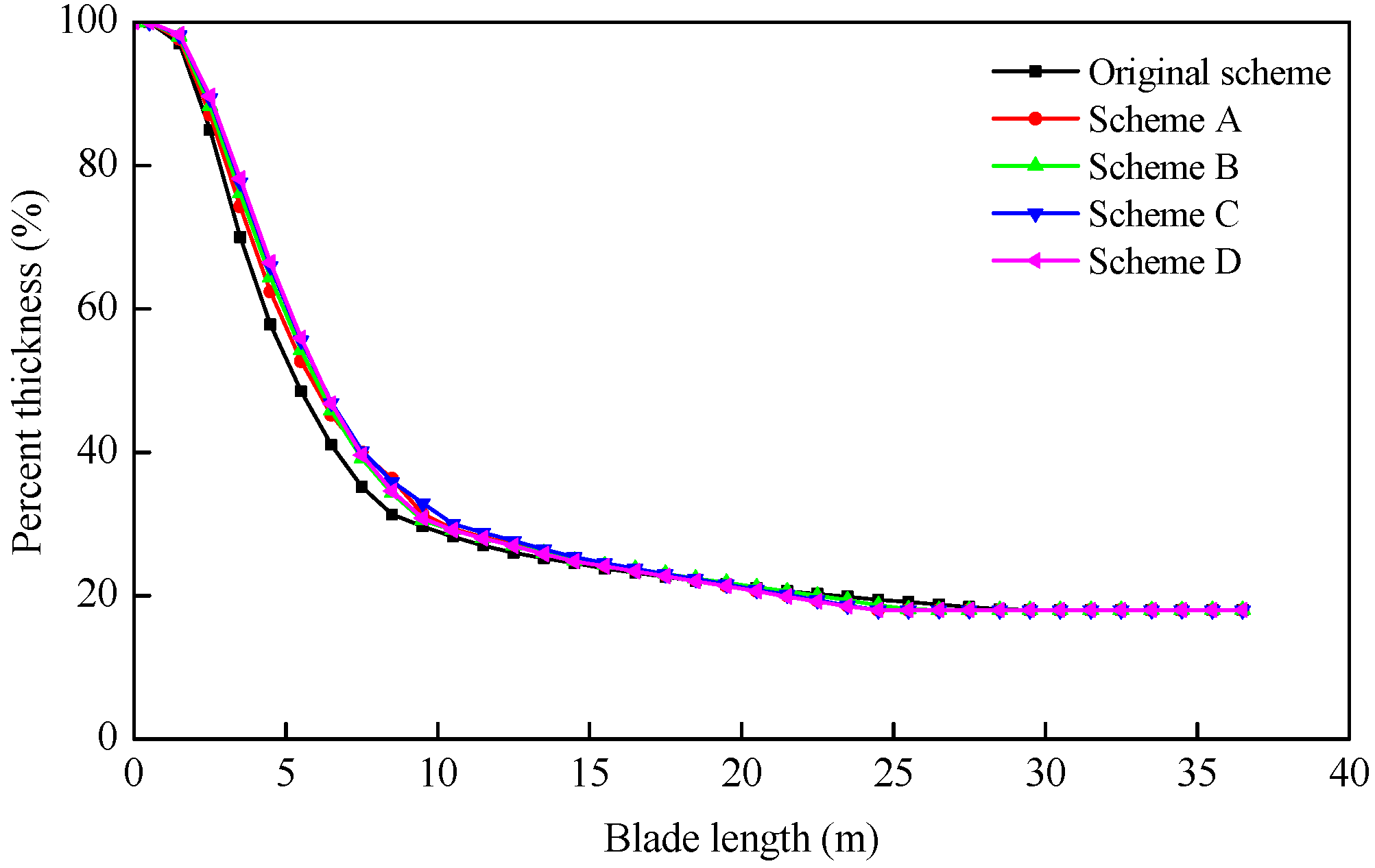
| Parameter | Original Scheme | Scheme A | Scheme B | Scheme C | Scheme D | Unit |
|---|---|---|---|---|---|---|
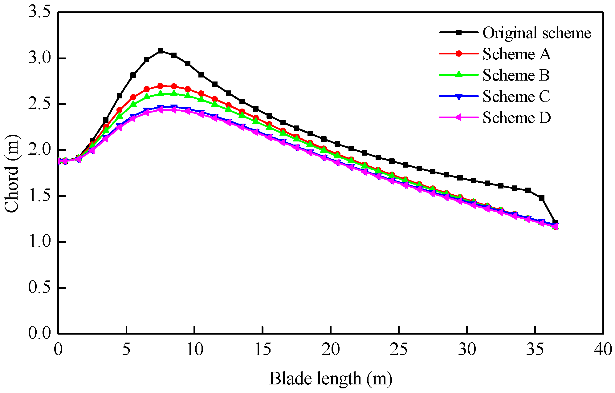
| x1 | 3.08 | 2.70 | 2.60 | 2.47 | 2.44 | m |
| x2 | 2.88 | 2.64 | 2.56 | 2.43 | 2.41 | m |
| x3 | 2.30 | 2.21 | 2.15 | 2.10 | 2.08 | m |
| x4 | 1.82 | 1.66 | 1.64 | 1.61 | 1.60 | m |
| x5 | 1.21 | 1.16 | 1.16 | 1.19 | 1.17 | m |
| x6 | 8.73 | 10.69 | 10.38 | 9.70 | 9.56 | ° |
| x7 | 6.64 | 6.72 | 6.61 | 6.59 | 6.60 | ° |
| x8 | 3.14 | 3.84 | 3.49 | 3.80 | 3.58 | ° |
| x9 | 0.43 | 0.85 | 0.82 | 0.88 | 0.97 | ° |
| x10 | −1.13 | −0.49 | −0.81 | −0.22 | 0.02 | ° |
| x11 | 6.75 | 7.73 | 6.96 | 7.10 | 7.03 | m |
| x12 | 9.50 | 9.81 | 9.32 | 10.51 | 9.73 | m |
| x13 | 14.10 | 14.18 | 14.32 | 14.34 | 14.21 | m |
| x14 | 28.95 | 24.32 | 25.16 | 24.35 | 24.20 | m |
| x15 | 19.0 | 15.5 | 15.6 | 15.2 | 14.9 | rpm |
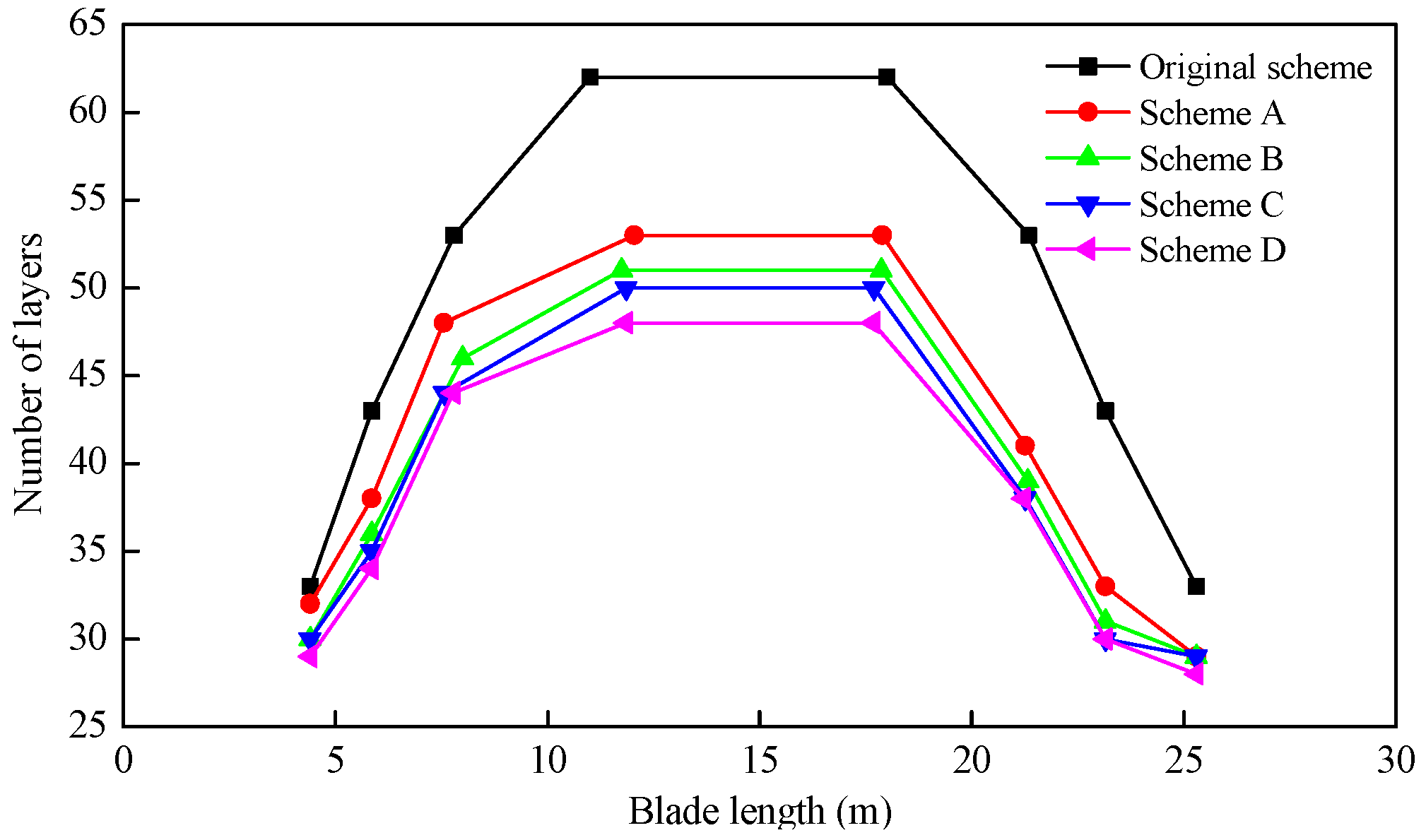
| x16 | 33 | 32 | 30 | 30 | 29 | - |
| x17 | 43 | 38 | 36 | 35 | 34 | - |
| x18 | 53 | 48 | 46 | 44 | 44 | - |
| x19 | 62 | 53 | 51 | 50 | 48 | - |
| x20 | 53 | 41 | 39 | 38 | 38 | - |
| x21 | 43 | 33 | 31 | 30 | 30 | - |
| x22 | 33 | 29 | 29 | 29 | 28 | - |
| x23 | 7.8 | 7.6 | 8.0 | 7.6 | 7.8 | m |
| x24 | 11.0 | 12.1 | 11.8 | 11.9 | 11.8 | m |
| x25 | 18.0 | 17.9 | 17.9 | 17.7 | 17.7 | m |
| x26 | 21.4 | 21.3 | 21.3 | 21.3 | 21.2 | m |
| x27 | 0.188 | 0.195 | 0.180 | 0.193 | 0.191 | m |
| x28 | 0.620 | 0.589 | 0.558 | 0.553 | 0.551 | m |


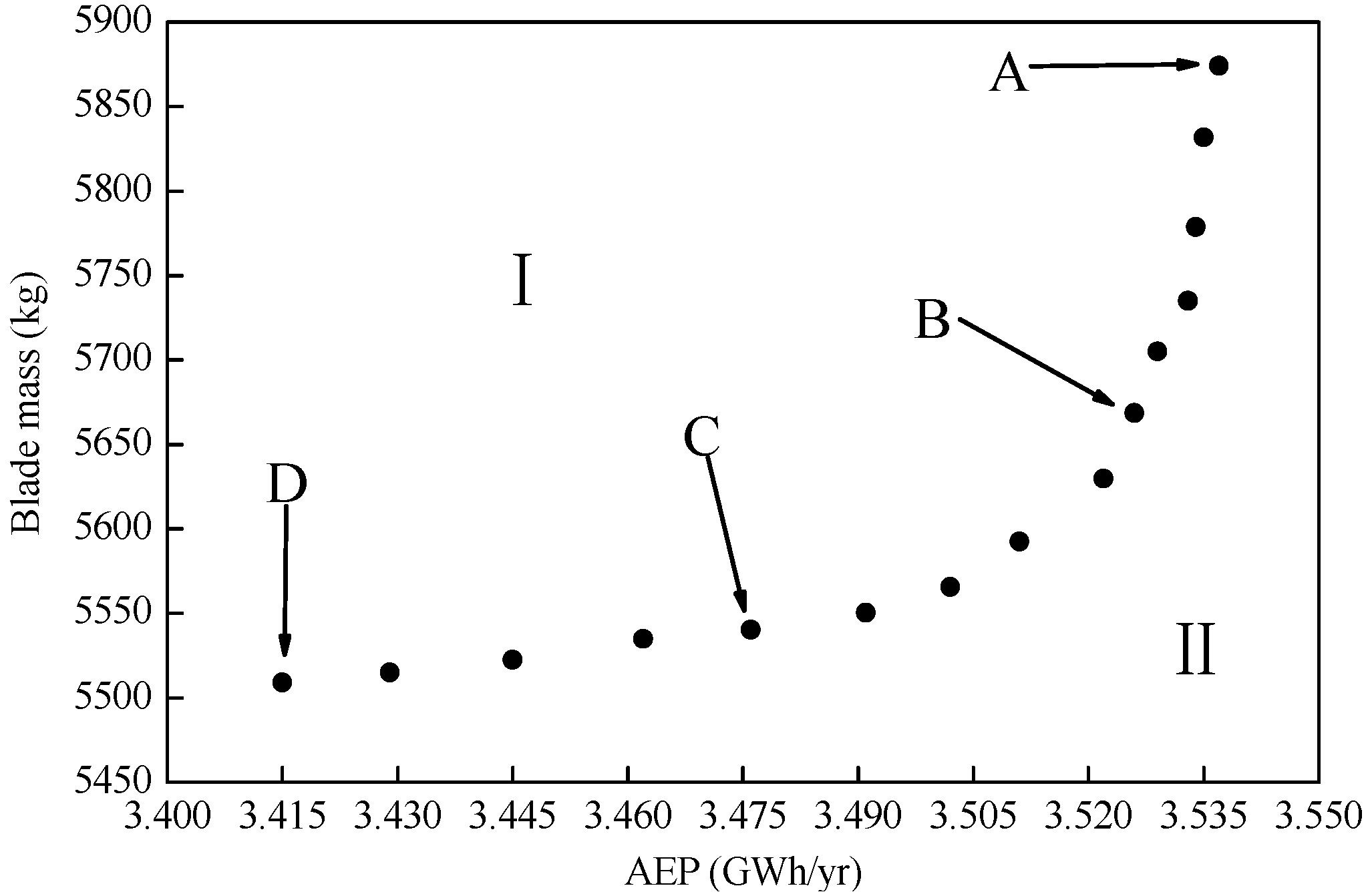
| Scheme | AEP (GWh/Year) | Blade Mass (kg) | Maximum Strain | Maximum Tip Deflection (m) | The Lowest Buckling Eigenvalue | The First Natural Frequency (Hz) |
|---|---|---|---|---|---|---|
| Original | 3.175 | 6555.2 | 0.00429 | 4.60 | 2.024 | 1.027 |
| A | 3.537 | 5874.1 | 0.00481 | 4.13 | 1.491 | 0.969 |
| B | 3.524 | 5668.4 | 0.00485 | 4.36 | 1.358 | 0.938 |
| C | 3.476 | 5550.3 | 0.00491 | 4.75 | 1.252 | 0.907 |
| D | 3.415 | 5509.1 | 0.00498 | 4.92 | 1.216 | 0.884 |
6. Conclusions
Acknowledgments
Author Contributions
Conflicts of Interest
References
- BTM Consult. World Wind Energy Market Update 2015; BTM Consult: Chicago, IL, USA, 2015. [Google Scholar]
- Burton, T.; Jenkins, N.; Sharpe, D.; Bossanyi, E. Wind Energy Handbook; John Wiley & Sons: Chichester, West Sussex, UK, 2011. [Google Scholar]
- Kim, B.; Kim, W.; Lee, S.; Bae, S.; Lee, Y. Developement and verification of a performance based optimal design software for wind turbine blades. Renew. Energy 2013, 54, 166–172. [Google Scholar] [CrossRef]
- Xudong, W.; Shen, W.Z.; Zhu, W.J.; Sørensen, J.N.; Jin, C. Shape optimization of wind turbine blades. Wind Energy 2009, 12, 781–803. [Google Scholar] [CrossRef]
- Kusiak, A.; Zheng, H. Optimization of wind turbine energy and power factor with an evolutionary computation algorithm. Energy 2010, 35, 1324–1332. [Google Scholar] [CrossRef]
- Sharifi, A.; Nobari, M.R. Prediction of optimum section pitch angle distribution along wind turbine blades. Energ. Convers. Manag. 2013, 67, 342–350. [Google Scholar] [CrossRef]
- Maalawi, K.Y.; Badr, M.A. Frequency optimization of a wind turbine blade in pitching motion. P. I. Mech. Eng. A 2010, 224, 545–554. [Google Scholar] [CrossRef]
- Dal Monte, A.; Castelli, M.R.; Benini, E. Multi-objective structural optimization of a HAWT composite blade. Compos. Struct. 2013, 106, 362–373. [Google Scholar] [CrossRef]
- Chen, J.; Wang, Q.; Shen, W.Z.; Pang, X.; Li, S.; Guo, X. Structural optimization study of composite wind turbine blade. Mater. Des. 2013, 46, 247–255. [Google Scholar] [CrossRef]
- Grujicic, M.; Arakere, G.; Pandurangan, B.; Sellappan, V.; Vallejo, A.; Ozen, M. Multidisciplinary design optimization for glass-fiber epoxy-matrix composite 5 MW horizontal-axis wind-turbine blades. J. Mater. Eng. Perform. 2010, 19, 1116–1127. [Google Scholar] [CrossRef]
- Bottasso, C.L.; Campagnolo, F.; Croce, A. Multi-disciplinary constrained optimization of wind turbines. Multibody Syst. Dyn. 2012, 27, 21–53. [Google Scholar] [CrossRef]
- Benini, E.; Toffolo, A. Optimal design of horizontal-axis wind turbines using blade-element theory and evolutionary computation. J. Sol. Energ. 2002, 124, 357–363. [Google Scholar] [CrossRef]
- Wang, L.; Wang, T.G.; Luo, Y. Improved non-dominated sorting genetic algorithm (NSGA)-II in multi-objective optimization studies of wind turbine blades. Appl. Math. Mech Engl. 2011, 32, 739–748. [Google Scholar] [CrossRef]
- Wang, T.; Wang, L.; Zhong, W.; Xu, B.; Chen, L. Large-scale wind turbine blade design and aerodynamic analysis. Chin. Sci. Bull. 2012, 57, 466–472. [Google Scholar] [CrossRef]
- Cai, X.; Zhu, J.; Pan, P.; Gu, R. Structural optimization design of horizontal-axis wind turbine blades using a particle swarm optimization algorithm and finite element method. Energies 2012, 5, 4683–4696. [Google Scholar] [CrossRef]
- Cairns, D.S.; Mandell, J.; Combs, D.C.; Rabern, D.A.; van Luchene, R.D. Analysis of a Composite Blade Design for the AOC 15/50 Wind Turbine Using a Finite Element Model; Sandia National Laboratories: Albuquerque, NM, USA, 2001.
- Locke, J.; Valencia, U.; Ishikawa, K. Design studies for twist-coupled wind turbine blades. In Proceedings of the ASME 2003 Wind Energy Symposium, Reno, NV, USA, 6–9 January 2003; American Society of Mechanical Engineers: Wichita, KS, USA, 2003; pp. 324–331. [Google Scholar]
- Spera, D.A. Wind Turbine Technology; American Society of Mechanical Engineers: Fairfield, NJ, USA, 1994. [Google Scholar]
- Gasch, R.; Twele, J. Wind Power Plants: Fundamentals, Design, Construction and Operation; Springer Science & Business Media: Berlin, Germany, 2011. [Google Scholar]
- Hansen, M.O. Aerodynamics of Wind Turbines; Routledge: New York, NY, USA, 2015. [Google Scholar]
- Ashwill, T.D. Cost Study for Large Wind Turbine Blades: WindPACT Blade System Design Studies (No. SAND2003-1428); Sandia National Labs.: Albuquerque, NM, USA; Livermore, CA, USA, 2003.
- Buckney, N.; Pirrera, A.; Green, S.D.; Weaver, P.M. Structural efficiency of a wind turbine blade. Thin-Wall Struct. 2013, 67, 144–154. [Google Scholar] [CrossRef]
- Lee, Y.J.; Jhan, Y.T.; Chung, C.H. Fluid-structure interaction of FRP wind turbine blades under aerodynamic effect. Compos. Part B 2012, 43, 2180–2191. [Google Scholar] [CrossRef]
- Liao, C.C.; Zhao, X.L.; Xu, J.Z. Blade layers optimization of wind turbines using FAST and improved PSO algorithm. Renew. Energy 2012, 42, 227–233. [Google Scholar] [CrossRef]
- Jureczko, M.E.; Pawlak, M.; Mężyk, A. Optimisation of wind turbine blades. J. Mater. Proc. Technol. 2005, 167, 463–471. [Google Scholar] [CrossRef]
- Deb, K.; Pratap, A.; Agarwal, S.; Meyarivan, T. A fast and elitist multiobjective genetic algorithm: NSGA-II. IEEE Trans. Evol. Comput. 2002, 6, 182–197. [Google Scholar] [CrossRef]
- Serrano, V.; Alvarado, M.; Coello, C.A. Optimization to manage supply chain disruptions using the NSGA-II. In Theoretical Advances and Applications of Fuzzy Logic and Soft Computing; Springer: Berlin/Heidelberg, Germany, 2007; pp. 476–485. [Google Scholar]
- Palanikumar, K.; Latha, B.; Senthilkumar, V.S.; Karthikeyan, R. Multiple performance optimization in machining of GFRP composites by a PCD tool using non-dominated sorting genetic algorithm (NSGA-II). Metal Mater. Int. 2009, 15, 249–258. [Google Scholar] [CrossRef]
- Zhu, J.; Cai, X.; Pan, P.; Gu, R. Multi-objective structural optimization design of horizontal-axis wind turbine blades using the non-dominated sorting genetic algorithm II and finite element method. Energies 2014, 7, 988–1002. [Google Scholar] [CrossRef]
© 2016 by the authors; licensee MDPI, Basel, Switzerland. This article is an open access article distributed under the terms and conditions of the Creative Commons by Attribution (CC-BY) license (http://creativecommons.org/licenses/by/4.0/).
Share and Cite
Zhu, J.; Cai, X.; Gu, R. Aerodynamic and Structural Integrated Optimization Design of Horizontal-Axis Wind Turbine Blades. Energies 2016, 9, 66. https://doi.org/10.3390/en9020066
Zhu J, Cai X, Gu R. Aerodynamic and Structural Integrated Optimization Design of Horizontal-Axis Wind Turbine Blades. Energies. 2016; 9(2):66. https://doi.org/10.3390/en9020066
Chicago/Turabian StyleZhu, Jie, Xin Cai, and Rongrong Gu. 2016. "Aerodynamic and Structural Integrated Optimization Design of Horizontal-Axis Wind Turbine Blades" Energies 9, no. 2: 66. https://doi.org/10.3390/en9020066
APA StyleZhu, J., Cai, X., & Gu, R. (2016). Aerodynamic and Structural Integrated Optimization Design of Horizontal-Axis Wind Turbine Blades. Energies, 9(2), 66. https://doi.org/10.3390/en9020066