
Ice Storage Air-Conditioning System Simulation with Dynamic Electricity Pricing: A Demand Response Study

Abstract
:1. Introduction
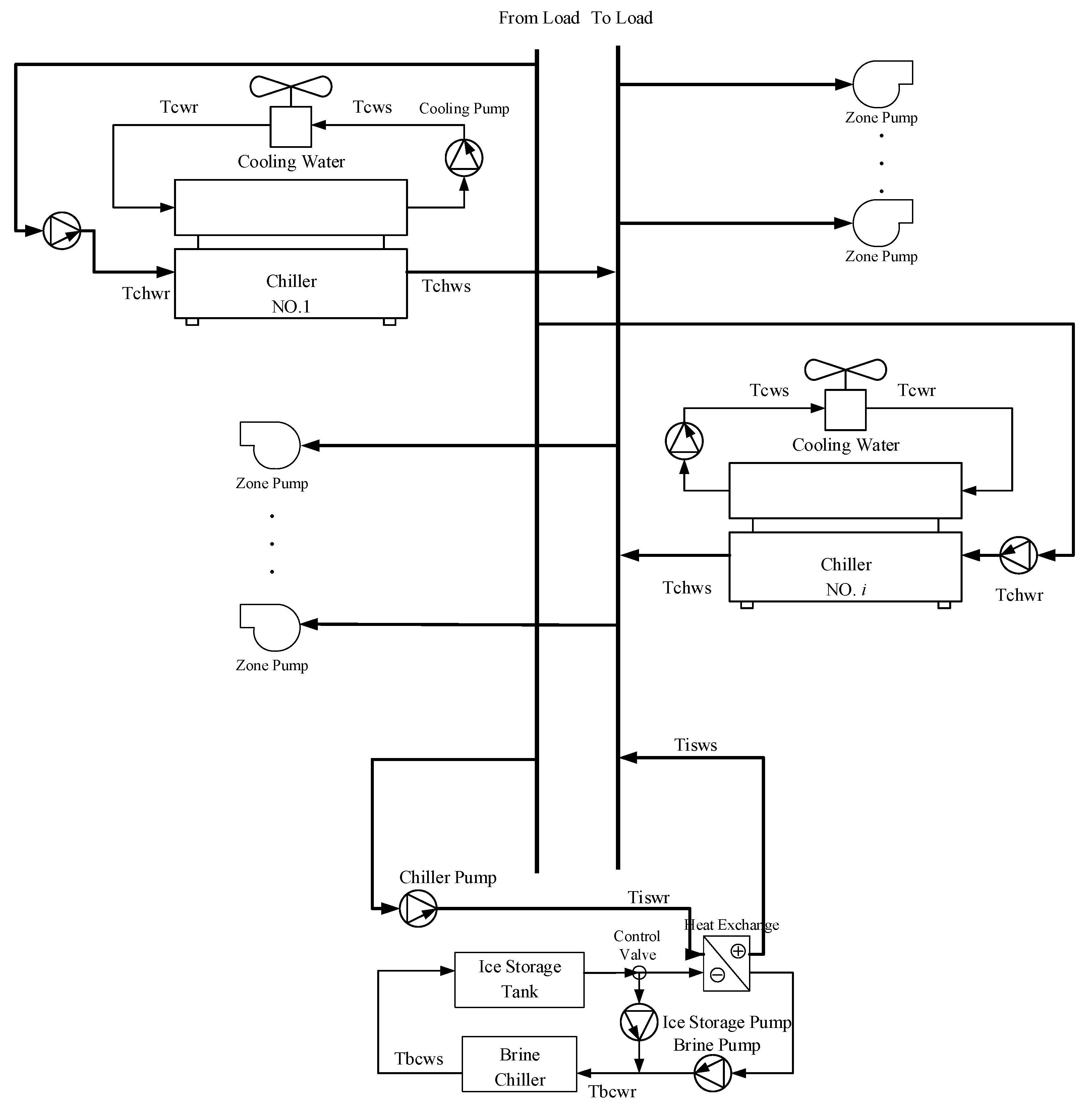
2. System Structure
2.1. Chiller Capacity Cooling Load
- : temperature difference of chilled water (°C)
- : the return temperature of chilled water (°C)
- : the supply temperature of chilled water (°C)
- : the flow rate of chilled water (L/min)
- : the density of chilled water (1 kg/m3)
- : the specific heat of chilled water (4.186 kJ/kg·K)
- : the cooling load of the ith chiller (kJ/h).
2.2. Ice Storage Cooling System
- : the temperature difference of ice storage water (°C)
- : the return temperature of ice storage water (°C)
- : the supply temperature of ice storage water (°C)
- LPM: the flow rate of ice storage water (L/min)
- : cooling load capacity of ice storage tank (kJ/h).
2.3. Ice Storage Air-Conditioning System
3. Proposed Methodology
3.1. Forager Bees
3.2. Onlooker Bees
3.3. Scout Bees
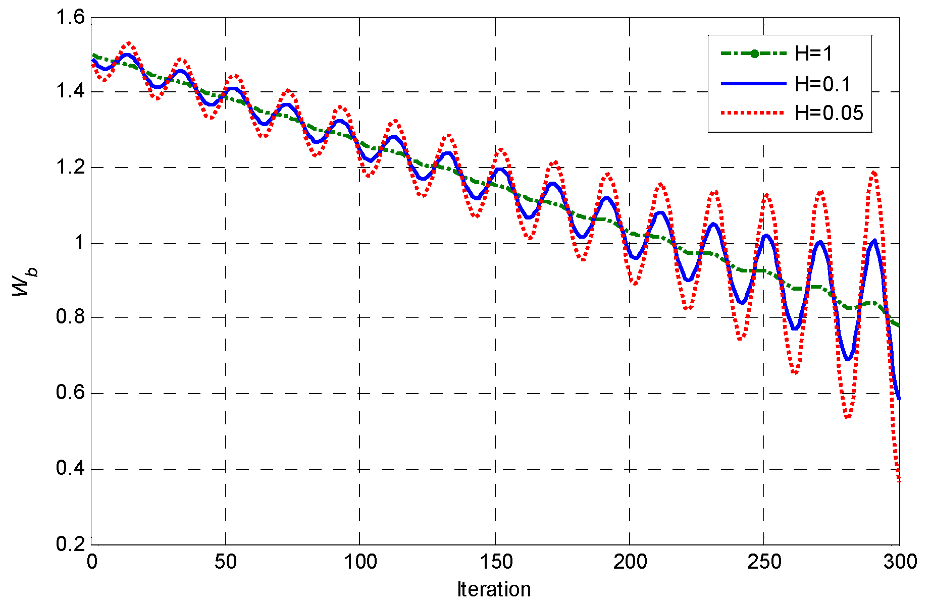
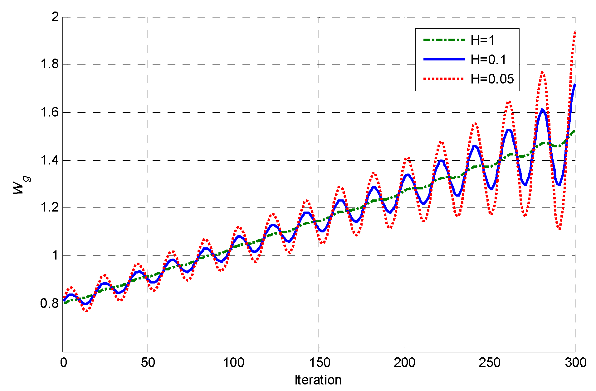
3.4. Self-Adaptation Repulsion Factor of Bee Swarm
| if comes from |
| if , then and |
| otherwise |
| if , then and |
| otherwise comes from |
| if , then and |
| otherwise |
| if , then and |
| end |
4. Simulation Results
4.1. Dynamic Electricity Price and Ice Storage Tank Strategy for Case Study
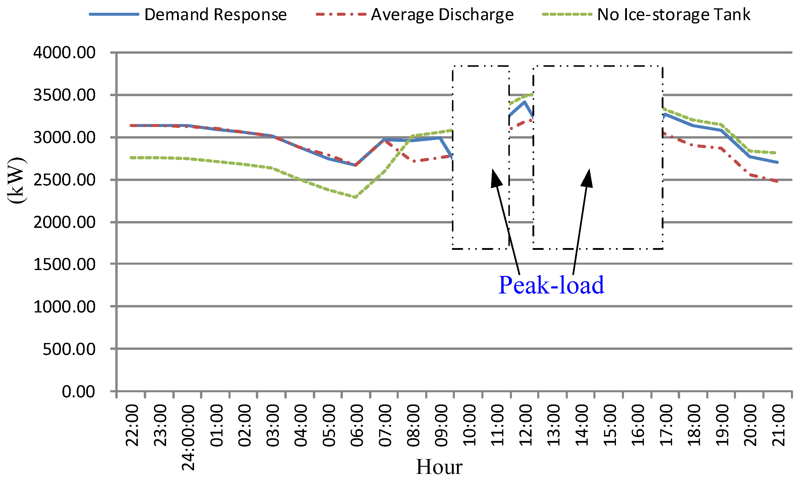
4.2. Simulation of Demand Response
5. Conclusions
Acknowledgments
Author Contributions
Conflicts of Interest
References
- Chua, K.J.; Chou, S.K.; Yang, W.M.; Yan, J. Achieving better energy-efficient air conditioning—A review of technologies and strategies. Appl. Energy 2013, 104, 87–104. [Google Scholar] [CrossRef]
- Yan, C.; Xue, X.; Wang, S.; Cui, B. A novel air-conditioning system for proactive power demand response to smart grid. Energy Convers. Manag. 2015, 102, 239–246. [Google Scholar] [CrossRef]
- Sanaye, S.; Shirazi, A. Thermo-economic optimization of an ice thermal energy storage system for air-conditioning applications. Energy Build. 2013, 60, 100–109. [Google Scholar] [CrossRef]
- The Taiwan Power Company (TPC). Time-of-Use Rate for Cogenerator Plants; The Electricity Rate Structure for Taipower Company: Taipei, Taiwan, 2014. [Google Scholar]
- Chassin, D.P.; Stoustrup, J.; Agathoklis, P.; Djilali, N. A new thermostat for real-time price demand response: Cost comfort and energy impacts of discrete-time control without deadband. Appl. Energy 2015, 155, 816–825. [Google Scholar] [CrossRef]
- Braun, J.E.; Kleni, S.A.; Mitchell, J.W.; Beckman, W.A. Applications of optimal control to chilled water systems without storage. ASHRAE Trans. 1989, 95, 663–675. [Google Scholar]
- Lee, W.S.; Chen, Y.T.; Wu, T.H. Optimization for ice-storage air-conditioning system using swarm algorithm. Appl. Energy 2009, 86, 1589–1595. [Google Scholar] [CrossRef]
- Sehar, F.; Rahman, S.; Pipattanasomporn, M. Impacts of ice storage on electrical energy consumptions in office buildings. Energy Build. 2012, 51, 255–262. [Google Scholar] [CrossRef]
- Sebzali, M.J.; Rubini, P.A. The impact of using chilled water storage systems on the performance of air cooled chillers in Kuwait. Energy Build. 2007, 39, 975–984. [Google Scholar] [CrossRef]
- Sebzali, M.J.; Rubini, P.A. Analysis of ice cool thermal storage for a clinic building in Kuwait. Energy Convers. Manag. 2006, 47, 3417–3434. [Google Scholar] [CrossRef]
- Chan, A.L.S.; Chow, T.T.; Fong, S.K.F.; Lin, J.Z. Performance evaluation of district cooling plant with ice storage. Energy 2006, 31, 2750–2762. [Google Scholar] [CrossRef]
- Vo, D.N.; Ongsakul, W. Economic dispatch with multiple fuel types by enhanced augmented Lagrange Hopfield network. Appl. Energy 2012, 91, 281–289. [Google Scholar] [CrossRef]
- Alsumait, J.S.; Sykulski, J.K.; Al-Othman, A.K. A hybrid GA–PS–SQP method to solve power system valve-point economic dispatch problems. Appl. Energy 2010, 87, 1773–1781. [Google Scholar] [CrossRef]
- Sinha, N.; Chakrabarti, R.; Chattopadhyay, P.K. Evolutionary programming techniques for economic load dispatch. IEEE Trans. Evolut. Comput. 2003, 7, 83–94. [Google Scholar] [CrossRef]
- Jahanbani Ardakani, A.; Fattahi Ardakani, F.; Hosseinian, S.H. A novel approach for optimal chiller loading using particle swarm optimization. Energy Build. 2008, 40, 2177–2187. [Google Scholar] [CrossRef]
- Lee, W.S.; Lin, L.C. Optimal chiller loading by particle swarm algorithm for reducing energy consumption. Appl. Therm. Eng. 2009, 29, 1730–1734. [Google Scholar] [CrossRef]
- Wang, X.; Dennis, M.; Hou, L. Clathrate hydrate technology for cold storage in air conditioning systems. Renew. Sustain. Energy Rev. 2014, 36, 34–51. [Google Scholar] [CrossRef]
- Chen, H.J.; Wang, W.P.; Chen, S.L. Optimization of an ice-storage air conditioning system using dynamic programming method. Appl. Therm. Eng. 2005, 25, 461–472. [Google Scholar] [CrossRef]
- Behnam, M.I.; Abbas, R.; Mehdi, E. Time-varying acceleration coefficients IPSO for solving dynamic economic dispatch with non-smooth cost function. Energy Convers. Manag. 2012, 56, 175–183. [Google Scholar]
- Ratnaweera, A.; Halgamuge, S.; Watson, H.C. Self-organizing hierarchical particle swarm optimizer with time-varying acceleration coefficients. IEEE Trans. Evolut. Comput. 2004, 8, 240–255. [Google Scholar] [CrossRef]
- Niknam, T.; Golestaneh, F. Enhanced bee swarm optimization algorithm for dynamic economic dispatch. IEEE Syst. J. 2013, 7, 754–762. [Google Scholar] [CrossRef]
- Taher, N.; Seyed, I.T.; Jamshid, A.; Sajad, T.; Majid, N. A modified honey bee mating optimization algorithm for multiobjective placement of renewable energy resources. Appl. Energy 2011, 88, 4817–4830. [Google Scholar]


| Hours | Load Classification | Ice Storage Tank | Chiller Prices (NT$) | |
|---|---|---|---|---|
| Process | Prices (NT$) | |||
| 22:00 | Off-Peak | Charging | 0.942 | 1.57 |
| 23:00 | Off-Peak | Charging | 0.942 | 1.57 |
| 24:00 | Off-Peak | Charging | 0.942 | 1.57 |
| 01:00 | Off-Peak | Charging | 0.942 | 1.57 |
| 02:00 | Off-Peak | Charging | 0.942 | 1.57 |
| 03:00 | Off-Peak | Charging | 0.942 | 1.57 |
| 04:00 | Off-Peak | Charging | 0.942 | 1.57 |
| 05:00 | Off-Peak | Charging | 0.942 | 1.57 |
| 06:00 | Off-Peak | Charging | 0.942 | 1.57 |
| 07:00 | Off-Peak | Charging | 0.942 | 1.57 |
| 08:00 | Partial-Peak | Discharging | 3.13 | 3.13 |
| 09:00 | Partial-Peak | Discharging | 3.13 | 3.13 |
| 10:00 | Peak | Discharging | 4.73 | 4.73 |
| 11:00 | Peak | Discharging | 4.73 | 4.73 |
| 12:00 | Partial-Peak | Discharging | 3.13 | 3.13 |
| 13:00 | Peak | Discharging | 4.73 | 4.73 |
| 14:00 | Peak | Discharging | 4.73 | 4.73 |
| 15:00 | Peak | Discharging | 4.73 | 4.73 |
| 16:00 | Peak | Discharging | 4.73 | 4.73 |
| 17:00 | Partial-Peak | Discharging | 3.13 | 3.13 |
| 18:00 | Partial-Peak | Discharging | 3.13 | 3.13 |
| 19:00 | Partial-Peak | Discharging | 3.13 | 3.13 |
| 20:00 | Partial-Peak | Discharging | 3.13 | 3.13 |
| 21:00 | Partial-Peak | Discharging | 3.13 | 3.13 |
| Chiller | ||||||
|---|---|---|---|---|---|---|
| Min on-time | 1 | 1 | 2 | 2 | 3 | 3 |
| Min off-time | 1 | 1 | 2 | 2 | 3 | 3 |
| SU(kW) | 30 | 30 | 40 | 40 | 50 | 50 |
| SD(kW) | 30 | 30 | 40 | 40 | 50 | 50 |
| Chiller Unit (kW) | (RT) | (RT) | ||||
|---|---|---|---|---|---|---|
| 65.777 | 0.689 | 1.694 × 10⁷ | 5.429 × 10⁸ | 165 | 550 | |
| 128.797 | 0.158 | 1.408 × 10³ | −1.142 × 10⁶ | 165 | 550 | |
| 81.407 | 0.423 | 6.317 × 10⁴ | −3.852 × 10⁷ | 300 | 1000 | |
| 107.725 | 0.433 | 2.510 × 10⁴ | −7.207 × 10⁸ | 300 | 1000 | |
| 623.209 | −1.602 | 2.821 × 10³ | −1.156 × 10⁶ | 300 | 1000 | |
| 101.536 | 0.299 | 8.498 × 10⁴ | −4.960 × 10⁷ | 300 | 1000 | |
| Ice Storage Tank Charge Process (kW) | ||||||
| 42.999 | 1.105 | −1.772 × 10³ | 1.252 × 10⁶ | 100 | 700 | |
| Ice Storage Tank Discharge Process (kW) | ||||||
| −2.256 | 0.071 | 5.485 × 10⁵ | −4.872 × 10⁸ | 105.26 | 1263.16 |
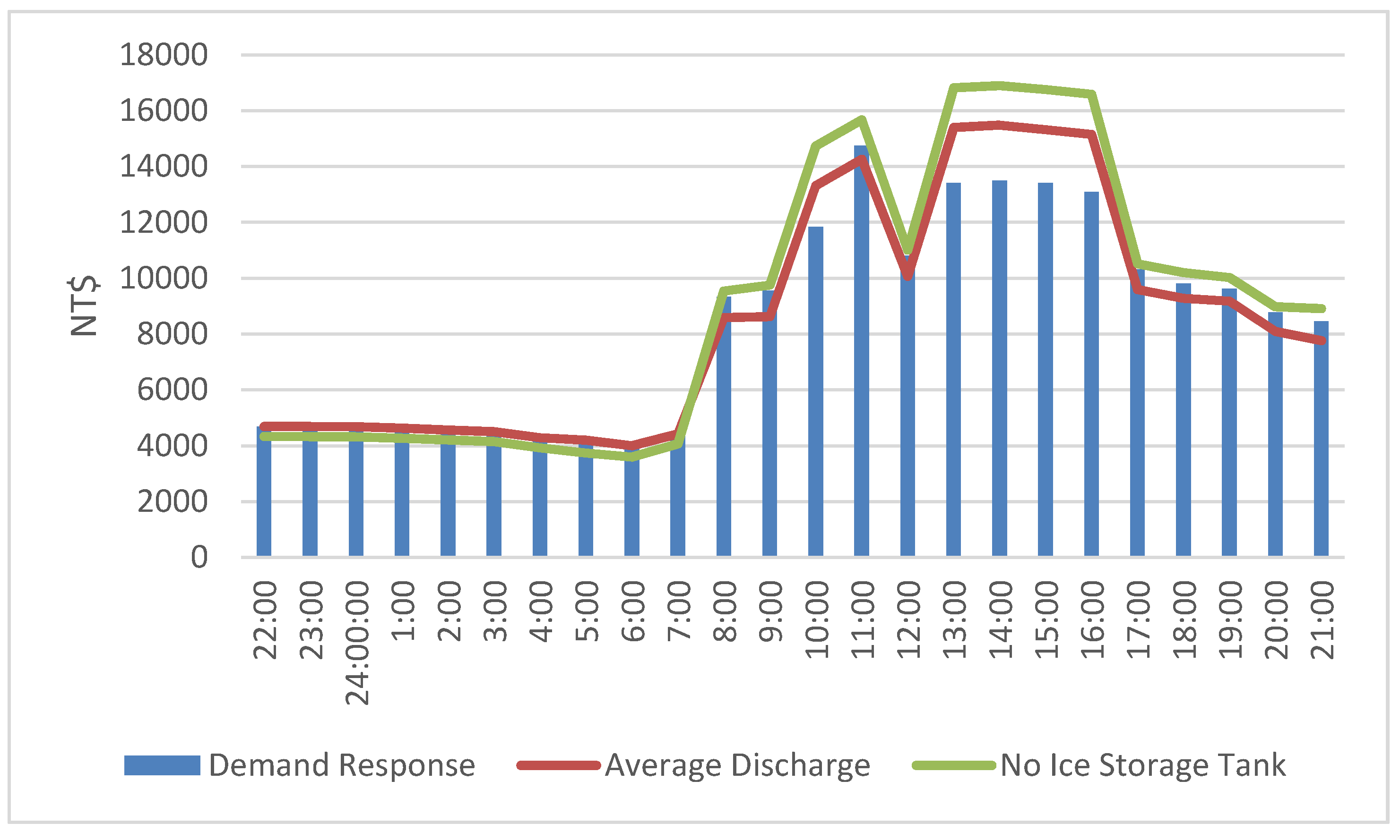
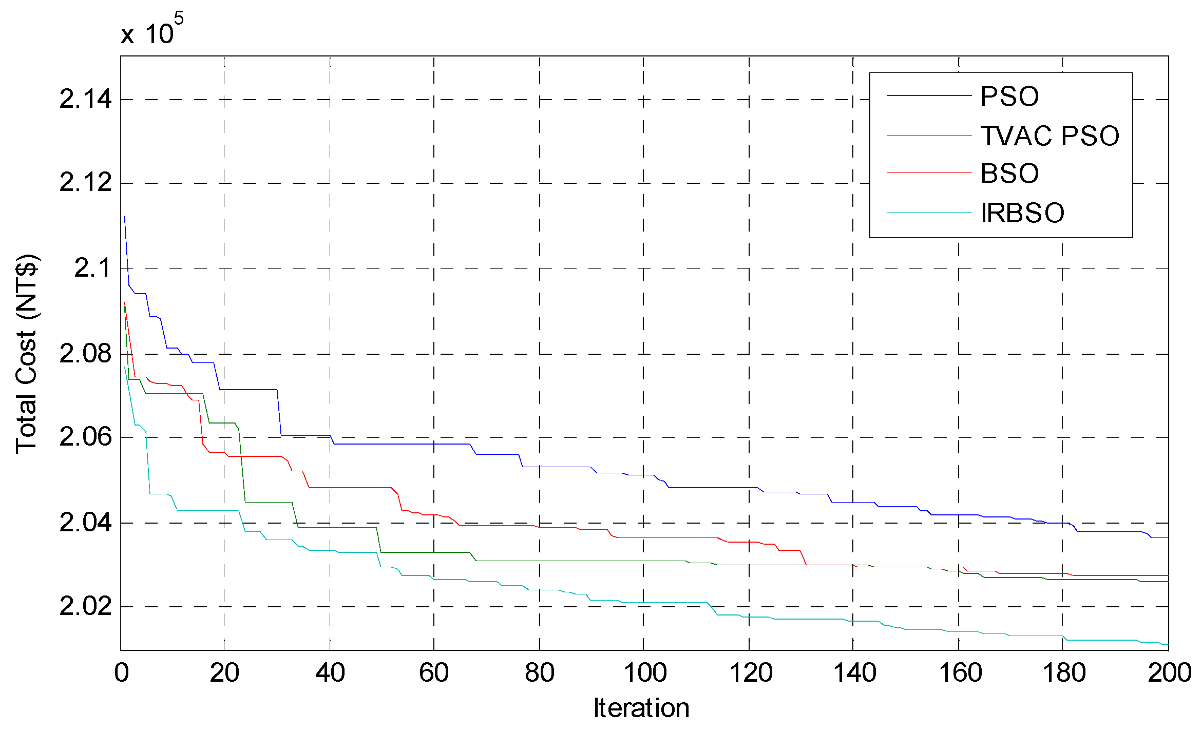
| Modeling Results | Total Cost (NT$) | |||
|---|---|---|---|---|
| PSO [17] | TVAC-PSO [21] | BSO [21] | IRBSO | |
| Demand Response | 203,641 | 202,615 | 202,754 | 201,142 |
| Average Discharge * | 207,341 | 206,072 | 206,162 | 204,741 |
| No Ice storage Tank | 218,648 | 217,861 | 217,874 | 217,298 |
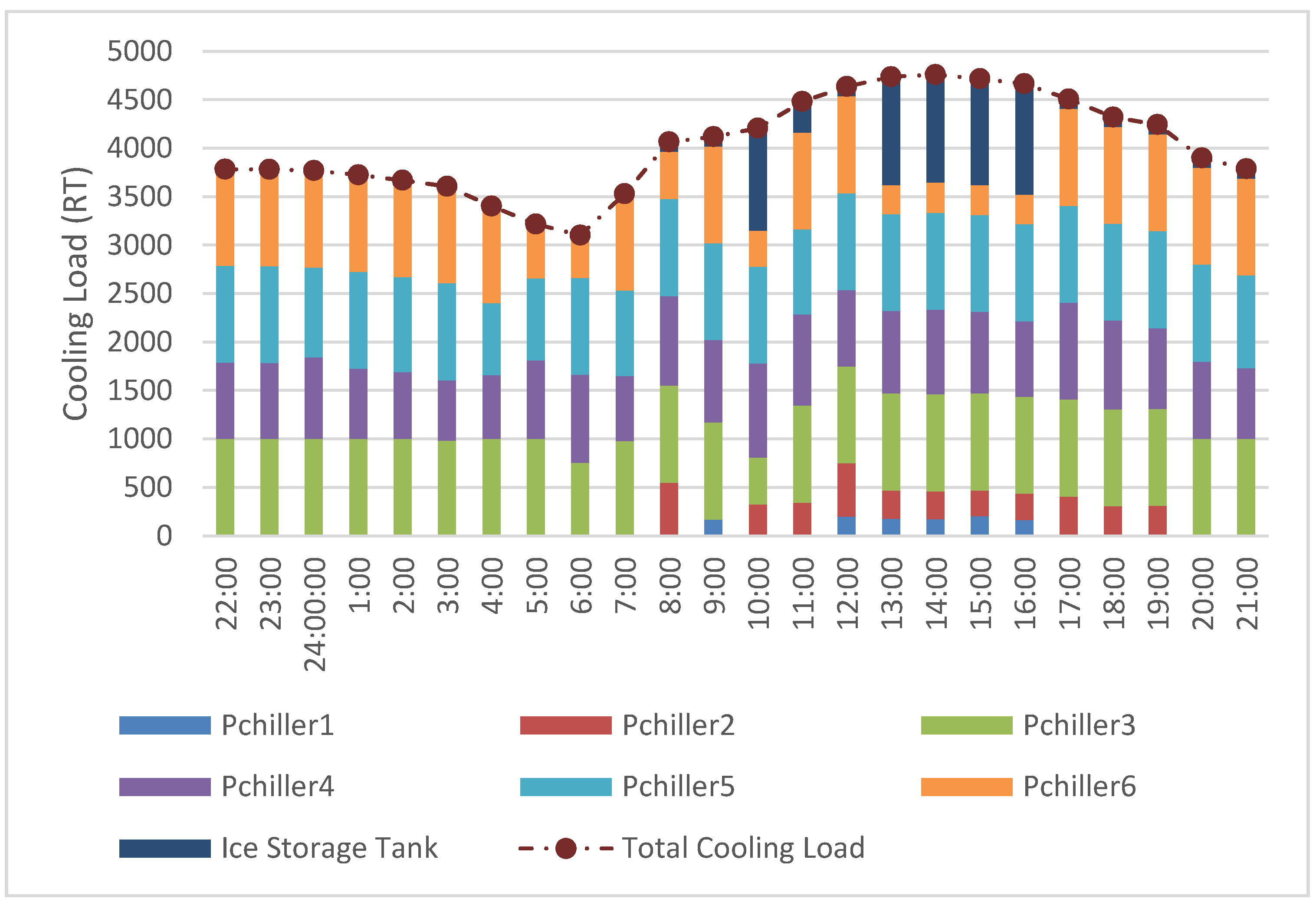
| Hours | Ice Storage Tank Cooling Load (RT) | Cooling Load of Chiller (RT) | Total Cooling Load (RT) | |||||
|---|---|---|---|---|---|---|---|---|
| Discharging | Pchiller,1 | Pchiller,2 | Pchiller,3 | Pchiller,4 | Pchiller,5 | Pchiller,6 | ||
| 22:00 | 0 | 0 | 0 | 1000.00 | 783.00 | 1000.00 | 1000.00 | 3783 |
| 23:00 | 0 | 0 | 0 | 1000.00 | 782.15 | 999.85 | 1000.00 | 3782 |
| 24:00 | 0 | 0 | 0 | 1000.00 | 798.92 | 972.08 | 1000.00 | 3771 |
| 01:00 | 0 | 0 | 0 | 1000.00 | 760.00 | 965.00 | 1000.00 | 3725 |
| 02:00 | 0 | 0 | 0 | 1000.00 | 680.87 | 988.13 | 1000.00 | 3669 |
| 03:00 | 0 | 0 | 0 | 1000.00 | 611.48 | 994.52 | 1000.00 | 3606 |
| 04:00 | 0 | 0 | 0 | 1000.00 | 629.19 | 773.81 | 1000.00 | 3403 |
| 05:00 | 0 | 499.76 | 0 | 440.21 | 921.86 | 1000.00 | 354.17 | 3216 |
| 06:00 | 0 | 0 | 0 | 720.77 | 916.90 | 983.37 | 481.96 | 3103 |
| 07:00 | 0 | 0 | 0 | 1000.00 | 568.55 | 962.45 | 1000.00 | 3531 |
| 08:00 | 475 | 0 | 293.57 | 1000.00 | 955.09 | 1000.00 | 342.34 | 4066 |
| 09:00 | 475 | 0 | 345.57 | 999.38 | 996.32 | 1000.00 | 303.74 | 4120 |
| 10:00 | 475 | 0 | 414.74 | 1000.00 | 994.66 | 1000.00 | 321.60 | 4206 |
| 11:00 | 475 | 0 | 254.31 | 1000.00 | 752.69 | 1000.00 | 1000.00 | 4482 |
| 12:00 | 475 | 267.44 | 460.44 | 1000.00 | 976.62 | 1000.00 | 456.50 | 4636 |
| 13:00 | 475 | 480.75 | 376.12 | 1000.00 | 967.31 | 1000.00 | 437.82 | 4737 |
| 14:00 | 475 | 165.00 | 281.12 | 1000.00 | 838.88 | 1000.00 | 1000.00 | 4760 |
| 15:00 | 475 | 379.96 | 550.00 | 1000.00 | 968.16 | 1000.00 | 344.88 | 4718 |
| 16:00 | 475 | 550.00 | 344.89 | 1000.00 | 983.67 | 1000.00 | 312.43 | 4666 |
| 17:00 | 475 | 0 | 225.44 | 1000.00 | 805.56 | 1000.00 | 1000.00 | 4506 |
| 18:00 | 475 | 193.67 | 0 | 1000.00 | 652.33 | 1000.00 | 1000.00 | 4321 |
| 19:00 | 475 | 0 | 450.70 | 1000.00 | 772.13 | 859.60 | 686.58 | 4244 |
| 20:00 | 475 | 0 | 0 | 1000.00 | 610.64 | 813.36 | 1000.00 | 3899 |
| 21:00 | 475 | 0 | 0 | 1000.00 | 582.00 | 731.00 | 1000.00 | 3788 |
| Total | 6650 | 2536.59 | 3996.90 | 23,160.36 | 19,308.99 | 23,043.15 | 18,042.01 | 96,738 |
| Hours | Cooling Load of Ice Storage Tank (RT) | Cooling Load of Chiller (RT) | Total Cooling Load (RT) | |||||
|---|---|---|---|---|---|---|---|---|
| Discharging | Pchiller,1 | Pchiller,2 | Pchiller,3 | Pchiller,4 | Pchiller,5 | Pchiller,6 | ||
| 22:00 | 0 | 0 | 0 | 1000.00 | 786.36 | 1000.00 | 996.64 | 3783 |
| 23:00 | 0 | 0 | 0 | 1000.00 | 782.00 | 1000.00 | 1000.00 | 3782 |
| 24:00 | 0 | 0 | 0 | 998.26 | 842.82 | 929.93 | 1000.00 | 3771 |
| 01:00 | 0 | 0 | 0 | 1000.00 | 725.00 | 1000.00 | 1000.00 | 3725 |
| 02:00 | 0 | 0 | 0 | 1000.00 | 688.88 | 983.58 | 996.54 | 3669 |
| 03:00 | 0 | 0 | 0 | 983.91 | 622.09 | 1000.00 | 1000.00 | 3606 |
| 04:00 | 0 | 0 | 0 | 1000.00 | 659.58 | 743.42 | 1000.00 | 3403 |
| 05:00 | 0 | 0 | 0 | 1000.00 | 809.21 | 848.97 | 557.82 | 3216 |
| 06:00 | 0 | 0 | 0 | 755.94 | 909.21 | 995.27 | 442.58 | 3103 |
| 07:00 | 0 | 0 | 0 | 978.68 | 669.39 | 882.93 | 1000.00 | 3531 |
| 08:00 | 100 | 0 | 550.00 | 1000.00 | 925.35 | 1000.00 | 490.65 | 4066 |
| 09:00 | 100 | 169.46 | 0 | 1000.00 | 850.54 | 1000.00 | 1000.00 | 4120 |
| 10:00 | 1057.726 | 0 | 325.62 | 482.74 | 968.98 | 1000.00 | 370.93 | 4206 |
| 11:00 | 319.6618 | 0 | 343.19 | 1000.00 | 944.07 | 875.07 | 1000.00 | 4482 |
| 12:00 | 100 | 197.53 | 550.00 | 1000.00 | 788.47 | 1000.00 | 1000.00 | 4636 |
| 13:00 | 1116.346 | 174.34 | 294.55 | 1000.00 | 851.77 | 1000.00 | 300.00 | 4737 |
| 14:00 | 1113.229 | 173.51 | 286.96 | 1000.00 | 874.95 | 1000.00 | 311.34 | 4760 |
| 15:00 | 1096.856 | 201.34 | 267.54 | 1000.00 | 843.24 | 1000.00 | 309.03 | 4718 |
| 16:00 | 1146.381 | 166.58 | 267.72 | 1000.00 | 780.58 | 1000.00 | 304.74 | 4666 |
| 17:00 | 100 | 0 | 406.00 | 1000.00 | 1000.00 | 1000.00 | 1000.00 | 4506 |
| 18:00 | 100 | 0 | 306.47 | 1000.00 | 914.53 | 1000.00 | 1000.00 | 4321 |
| 19:00 | 100 | 0 | 309.28 | 1000.00 | 834.72 | 1000.00 | 1000.00 | 4244 |
| 20:00 | 100 | 0 | 0 | 1000.00 | 799.00 | 1000.00 | 1000.00 | 3899 |
| 21:00 | 100 | 0 | 0 | 1000.00 | 730.04 | 957.96 | 1000.00 | 3788 |
| Total | 6650 | 1082.76 | 3907.34 | 23,199.52 | 19,600.77 | 23,217.13 | 19,080.27 | 96,738 |
| Hours | Process | Ice Storage (kW) | Chiller Capacity (kW) | SU & SD (kW) | Total (kW) | Total Cost (NT$) |
|---|---|---|---|---|---|---|
| 22:00 | Charging | 377.66 | 2757.33 | 0 | 3134.99 | 4684.76 |
| 23:00 | Charging | 377.66 | 2756.03 | 0 | 3133.69 | 4682.72 |
| 24:00 | Charging | 377.66 | 2754.67 | 0 | 3132.33 | 4680.59 |
| 01:00 | Charging | 377.66 | 2716.81 | 0 | 3094.47 | 4621.15 |
| 02:00 | Charging | 377.66 | 2680.94 | 0 | 3058.59 | 4564.82 |
| 03:00 | Charging | 377.66 | 2638.95 | 0 | 3016.60 | 4498.90 |
| 04:00 | Charging | 377.66 | 2502.73 | 0 | 2880.39 | 4285.04 |
| 05:00 | Charging | 377.66 | 2370.06 | 0 | 2747.71 | 4076.74 |
| 06:00 | Charging | 377.66 | 2290.54 | 0 | 2668.20 | 3951.90 |
| 07:00 | Charging | 377.66 | 2593.62 | 0 | 2971.28 | 4427.74 |
| 08:00 | Discharging | 5.32 | 2948.25 | 30 | 2953.57 | 9338.56 |
| 09:00 | Discharging | 5.32 | 2986.76 | 60 | 2992.08 | 9553.02 |
| 10:00 | Discharging | 76.31 | 2366.56 | 60 | 2442.87 | 11838.57 |
| 11:00 | Discharging | 24.38 | 3093.55 | 0 | 3117.93 | 14747.79 |
| 12:00 | Discharging | 5.32 | 3414.46 | 30 | 3419.79 | 10797.83 |
| 13:00 | Discharging | 77.32 | 2759.21 | 0 | 2836.54 | 13416.82 |
| 14:00 | Discharging | 77.29 | 2777.48 | 0 | 2854.77 | 13503.05 |
| 15:00 | Discharging | 77.07 | 2759.79 | 0 | 2836.86 | 13418.34 |
| 16:00 | Discharging | 77.56 | 2689.13 | 0 | 2766.68 | 13086.42 |
| 17:00 | Discharging | 5.32 | 3258.81 | 30 | 3264.13 | 10310.63 |
| 18:00 | Discharging | 5.32 | 3125.70 | 0 | 3131.02 | 9800.10 |
| 19:00 | Discharging | 5.32 | 3071.31 | 0 | 3076.63 | 9629.86 |
| 20:00 | Discharging | 5.32 | 2767.83 | 30 | 2773.16 | 8773.88 |
| 21:00 | Discharging | 5.32 | 2695.15 | 0 | 2700.47 | 8452.48 |
| Total | 4229.05 | 700.00 | 240 | 71,004.73 | 201,141.71 | |
| Modeling Results | Total Power (kW) | |||
|---|---|---|---|---|
| PSO [17] | TVAC-PSO [17] | BSO [18] | IRBSO | |
| Demand Response | 71,298 | 71,276 | 71,281 | 71,245 |
| Average Discharge | 71,403 | 71,382 | 71,393 | 71,182 |
| No Ice storage Tank | 71,618 | 71,609 | 71,613 | 71,549 |
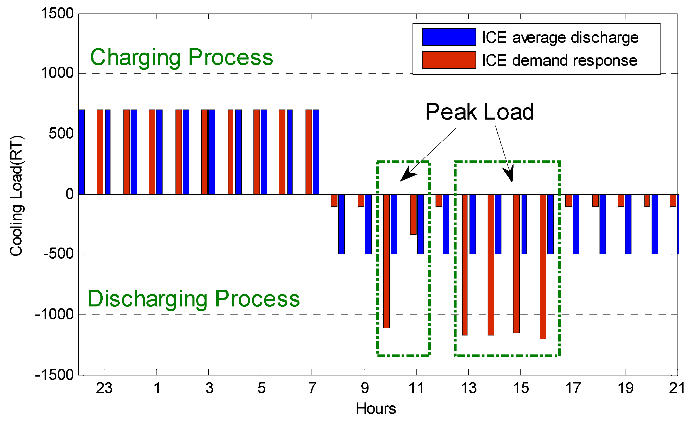
| IRBSO | Modeling Results | Max. Load of Peak (kW) | Average Load of Peak (kW) | Max. Load of Partial-Peak (kW) | Min. Off-Peak load (kW) | Load Range * (kW) |
|---|---|---|---|---|---|---|
| Summer | Demand Response | 3117.93 | 2809.27 | 3449.79 | 2668.20 | 449.73 |
| Average Discharge | 3273.08 | 3133.38 | 3185.26 | 2671.36 | 601.72 | |
| No Ice Storage Tank | 3572.16 | 3434.18 | 3484.64 | 2290.03 | 1282.13 |
© 2016 by the authors; licensee MDPI, Basel, Switzerland. This article is an open access article distributed under the terms and conditions of the Creative Commons by Attribution (CC-BY) license (http://creativecommons.org/licenses/by/4.0/).
Share and Cite
Lo, C.-C.; Tsai, S.-H.; Lin, B.-S. Ice Storage Air-Conditioning System Simulation with Dynamic Electricity Pricing: A Demand Response Study. Energies 2016, 9, 113. https://doi.org/10.3390/en9020113
Lo C-C, Tsai S-H, Lin B-S. Ice Storage Air-Conditioning System Simulation with Dynamic Electricity Pricing: A Demand Response Study. Energies. 2016; 9(2):113. https://doi.org/10.3390/en9020113
Chicago/Turabian StyleLo, Chi-Chun, Shang-Ho Tsai, and Bor-Shyh Lin. 2016. "Ice Storage Air-Conditioning System Simulation with Dynamic Electricity Pricing: A Demand Response Study" Energies 9, no. 2: 113. https://doi.org/10.3390/en9020113
APA StyleLo, C.-C., Tsai, S.-H., & Lin, B.-S. (2016). Ice Storage Air-Conditioning System Simulation with Dynamic Electricity Pricing: A Demand Response Study. Energies, 9(2), 113. https://doi.org/10.3390/en9020113