Article

Estimation of Energy Consumption and Greenhouse Gas Emissions of Transportation in Beef Cattle Production

1
Texas Institute for Applied Environmental Research, Tarleton State University, Stephenville, TX 76402, USA
2
Department of Agriculture and Consumer Sciences, Tarleton State University, Stephenville, TX 76402, USA
*
Author to whom correspondence should be addressed.
Energies 2016, 9(11), 960; https://doi.org/10.3390/en9110960
Submission received: 24 August 2016 / Revised: 7 November 2016 / Accepted: 11 November 2016 / Published: 18 November 2016

Abstract

:
Accounting for transportation is an important part of the life cycle analysis (LCA) of beef cattle production because it is associated with energy consumption and greenhouse gas emissions. This paper describes the development and application of a model that estimates energy consumption and greenhouse gas emissions of transport in beef cattle production. The animal transport model is based on the weight and number of animals in each weight category, type of trailer, vehicle, and fuel used. The energy consumption and greenhouse gas emission estimates of animal feed transportation are based on the weight of a truckload and the number of truckloads of feed transported. Our results indicate that a truckload is travelling approximately 326 km in connection with beef cattle production in the study region. The fuel consumption amounts to 24 L of fossil fuel per 1000 kg of boneless beef. The corresponding greenhouse gas emission is 83 kg. It appears from our results that the majority of energy consumption and greenhouse gas emissions are associated with sending the finished cattle to slaughterhouses and bringing feeder cattle to feedlots. Our results point out appreciable reductions in energy consumption and greenhouse gas emissions by changing from conventional fuel to bio-fuel.

1. Introduction

Beef cattle production is important in the United States from the standpoints of food production, export potential, and economic impact (a $44 billion industry) [1]. Although the production of beef is mainly driven by market forces, most producers wish to make sure beef cattle production is as eco-friendly as possible. In addition, consumers should be aware of the ecological consequences of beef cattle production.
About 50% of the total beef cattle and calf production in the United States occurs in Texas, Nebraska, Kansas, Oklahoma, and California [2,3], of which Texas, Kansas, and Oklahoma are in the Southern Great Plains (SGP). This outlines the importance of the SGP for beef cattle production in the nation. Because of this importance, and the vulnerability of animal production arising from changing climate, a five-year USDA-funded study titled “Resilience and vulnerability of beef cattle production in the Southern Great Plains under changing climate, land use, and markets” was initiated as a multi-institutional and multi-disciplinary collaboration involving four universities and three research centers [4]. The collaborating institutions include the Texas Institute for Applied Environmental Research (TIAER)—Tarleton State University, United States Department of Agriculture (USDA)—Agricultural Research Service (ARS) in El Reno, Oklahoma, USDA—ARS in Bushland, Texas, Kansas State University, Oklahoma State University, University of Oklahoma, and the Samuel R. Noble Foundation in Ardmore, Oklahoma.
The project goal is to safeguard and promote regional beef production while mitigating its environmental footprint. The project is focused on the vulnerability and resilience of beef cattle—forage—rangeland—winter wheat production system in the SGP under changing climate. Conducting a full Life Cycle Analysis (LCA) is one of the major objectives of the study, in addition to field experiments, extension, outreach, and education. Estimation of all inputs and outputs of water, energy, and greenhouse emissions in beef cattle production are parts of the LCA.
Accounting for transportation is an important part of the life cycle analysis of beef cattle production because it is associated with energy consumption and greenhouse gas emissions. Cattle are typically transported for getting fed and slaughtered. Animal feed is transported to feedlots. Given the nature of the beef industry, transporting cattle over long distances is unavoidable [5]. This is because of items such as (a) consistent demand for beef in the market (most of the slaughterhouses kill cattle six days a week and pack beef on all seven days of the week, however, calving occurs in specific seasons of the year); (b) animal feed availability; (c) lack/availability of slaughter facilities; and (d) variations in climate throughout the country.
Almost all beef cattle are transported more than once. For example, feeder calves might be transported from a ranch to a livestock auction market, order-buying station, backgrounding facility, pasture as a stocker, feedlot, and finally to a beef processing facility. Under the above assumptions, the calf could be transported six times during its life. Market cows and bulls are also shipped to numerous locations and often across long distances. They could be transported to a livestock auction market, a cattle-buying station, and finally a beef processing plant. This does not include multiple short-distance transportations between pastures within a single farm or ranch.
Currently, there are some tools available to estimate greenhouse gas emissions from vehicle operations. They are Greenhouse Gases, Regulated Emissions, and Energy Use in Transportation Model (GREET) [6] or Fleet Footprint Calculator [7]. MOVES (MOtor Vehicle Emission Simulator) is the United States Environmental Protection Agency’s (USEPA) current official model for estimating air pollution emissions from cars, trucks, and motorcycles. The National Mobile Inventory Model (NMIM) is another USEPA model developed to estimate current and future emission inventories for on-road vehicles and off-road equipment. Greenhouse Gas Emissions Model (GEM) for medium- and heavy-duty vehicle compliance is another USEPA model that estimates the greenhouse gas (GHG) emissions and fuel efficiency performance of specific aspects of heavy-duty vehicles. However, they do not specifically include scenarios on animal transport or animal feed transport into consideration. In addition, animal transport trailers and vehicle used to transport animals and animal feed vary widely depending on the scale of operation, requirement, frequency of use, and also affordability for the producer. Therefore, it warrants the development of a new tool with a focus on transportation scenarios in beef cattle production.
The new tool developed as a part of this study estimates energy consumption and greenhouse gas emissions based on a well-to-wheel (WTW) analysis [8,9]. There are two stages in WTW: well-to-pump (WTP) and pump-to-wheels (PTW). The WTP stage starts with the fuel feedstock recovery, followed by fuel production, and ends with the fuel available at the pump, while the PTW stage represents the vehicle's operating activities. It is important to examine transportation fuels and technologies on a WTW basis in order to properly compare alternatives, as activities upstream of vehicle operation can use significant amounts of energy and subsequently produce a large amount of emissions.
This manuscript deals with the estimation of energy consumption and greenhouse gas emissions associated with transportation in beef cattle production. The usefulness of the computer model developed for the present study and for other similar studies is demonstrated with data from southwestern Kansas, because of the following reasons: (1) vehicle miles transportation data on animal transport and animal feed transport is available from an extensive transportation logistic study on meat-related industries in southwestern Kansas [10]; (2) some of the counties in southwestern Kansas comes under the study area of “Resilience and vulnerability of beef cattle production in the Southern Great Plains under changing climate, land use, and markets” project; (3) southwestern Kansas has a large number of cattle feeding operations; and (4) Kansas has some large cattle slaughter facilities, with a total annual kill factor of around 35,000 head per day.

2. Materials and Methods

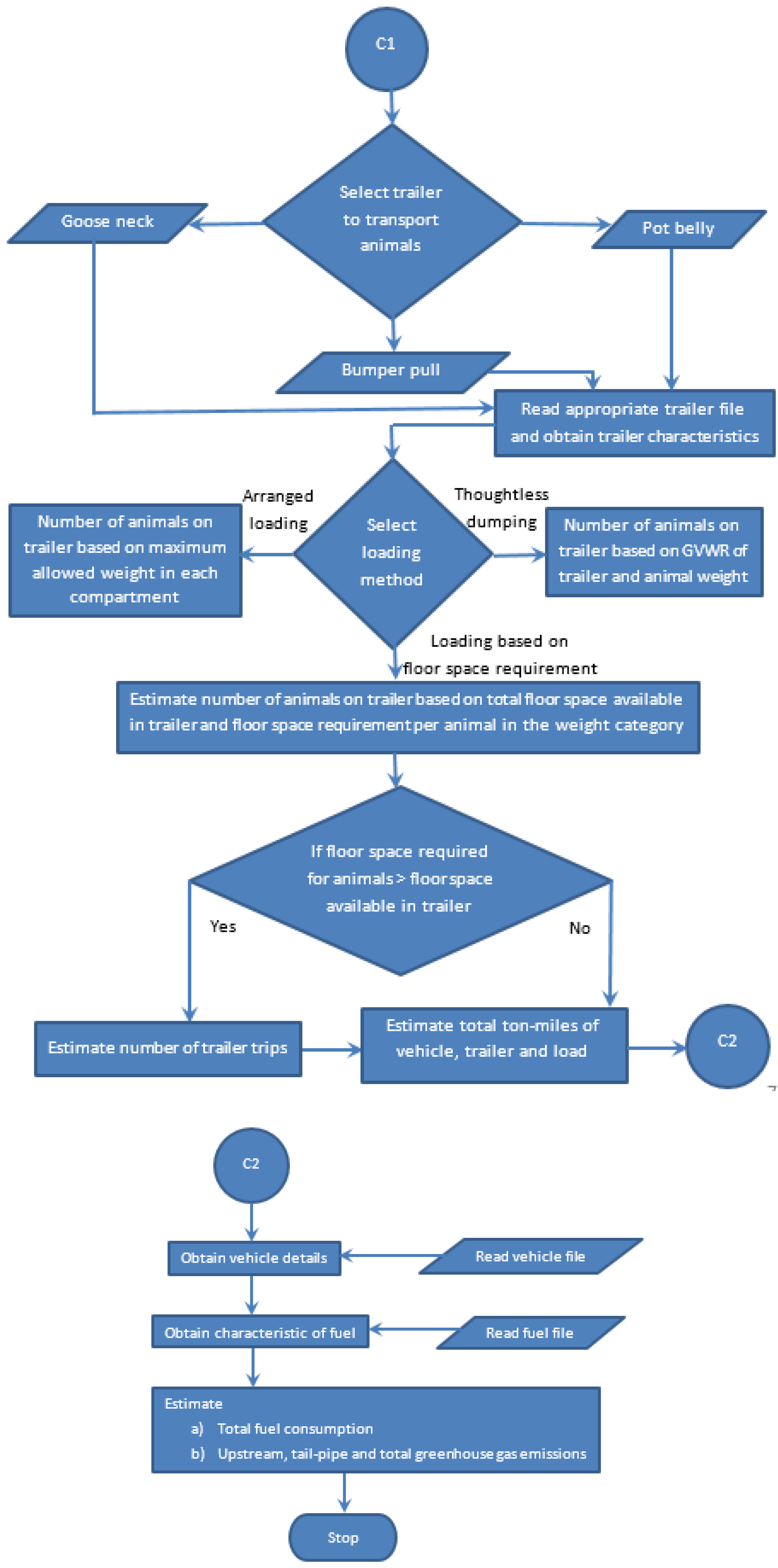
2.1. A Computer Model to Estimate Energy Requirements and Greenhouse Gas Emissions

A computer model is developed in FORTRAN to estimate the energy consumption and greenhouse emissions associated with transportation in beef cattle production. The computer model has one main program, which calls many sub-routines that carry out specific tasks. The model uses simple text files in free format for input. Output can be either printed on screen or sent to a text file. Currently, the model runs from command prompt. In the near future, the model will have a user interface. More details on the model and the sequence of computations are shown in Appendix A and an example calculation is demonstrated in Appendix B.

2.2. Databases Used

2.2.1. Trailer Database

The computer model developed uses a trailer database. The trailer database contains details on length and width of the trailer, Gross Vehicle Weight Rating (GVWR), empty weight, and floor space availability (to load the animals) of the trailer. Also included in the trailer file, are number of decks (if transporting smaller animals in multiple deck trailers, e.g., hogs) and the suggested truck to haul the trailer. The trailers are categorized based on three different hitch types, namely, pot belly (or possum belly), gooseneck, and bumper pull. Multiple trailer options are available within each hitch system. Four, 16, and seven different trailer types are available under pot belly, gooseneck, and bumper pull trailers, respectively. The differences in trailer types are based on differences in floor space to load animals and the weight allowed on the trailers [11,12]. The user selects the trailer based on length, width, and the GVWR. Pot belly trailers, in general, are used to transport many animals together (typically 30–45 finished animals or 50–75 feeder cattle) over long distances, typical to many large-scale commercial beef cattle operations. Bumper pull trailers, or drag along trailers, are the smallest among the animal trailers. Usually, a Sports Utility Vehicle (SUV) or Crossover Utility Vehicle (CUV) can pull them. Gooseneck trailers are smaller than pot belly but larger than bumper pull trailers. They are typically pulled by pickup trucks. Many of the gooseneck trailers qualify to be commercial trailers.

2.2.2. Vehicle Database

The model allows eight categories of truck/tractor, indicated by vehicle class. The vehicle classification system is adopted from Brown et al. [13]. The vehicles included in the database include passenger cars to large combination truck/tractors. Multiple categories are included for pickup trucks, based on the weight they can pull [14]. Two categories are included for large trucks that can haul 22 metric tons (or 50,000 lbs) of payload. The database has parameters on gross vehicle weight (including trailer weight and maximum payload allowed), empty weight of trailer, and maximum payload the vehicle can haul [14]. For each of the vehicle types, mileage and fuel consumption are separately available from Brown et al. [13]. The fuel consumption information is available per ton-mile (a ton-mile means a ton (U.S. short tons) of load hauled for a mile). The vehicle file information is based on Brown et al. [13]. In addition, freight trains are also specified in the model. Parameters similar to trucks are also included for freight trains, per car [15]. The purpose of including freight train information is to estimate the energy consumption and greenhouse gas emissions associated with the transport of animal feed and slaughterhouse waste.

2.2.3. Fuel Database

Many different types of fuels can be included in the model to estimate fuel consumption and greenhouse gas emissions in beef cattle production. They include gasoline, gasoline with ethanol blend, conventional diesel, bio-diesel, natural gas, ethanol, gaseous and liquid hydrogen, and electricity. Variations within a particular fuel (e.g., compressed natural gas, liquefied natural gas, liquefied landfill gas, and compressed landfill gas) are also included. The fuel database has parameters on energy content quantified in terms of low heat value (LHV) and high heat value (HHV) [7,16]. The other parameters include upstream and tailpipe greenhouse gas emissions factors, which are based on the Fleet Footprint Calculator model [7]. The fuel type can be selected by the user based on a unique code which identifies the fuel (e.g., LNG indicates liquefied natural gas).

2.3. Input Requirement from the User

The user needs to enter the number of categories of animals to be transported. Weight and number of animals in each category are needed. Distance transported is another parameter required from the user. The type of trailer used for transporting the animals (should be selected from the trailer database), type of vehicle selected for hauling the trailer (to be selected from the vehicle database), and the fuel used in the vehicle (to be selected from fuel database) are also needed. The model also requires two parameters on animal slaughter, namely, (a) proportion of live animal becoming carcass (dressing percentage) and (b) proportion of carcass becoming boneless beef. These two parameters are needed to quantify the energy consumption and greenhouse gas emissions per unit of beef (say, liter (L) of fuel required per kg of boneless beef). Finally, the user has the option of selecting one of the three possible cattle loading methods. The first method allows the number of animals in the trailer based on trailer GVWR (the maximum number of animals can be loaded using this option). This category is designated as a thoughtless loading option. The second method allows loading the animals in each compartment of the trailer based on a suggested maximum load in that compartment (e.g., the pot belly trailer has specific recommendations on loading for each compartment) [17]. This is indicated in the model as arranged loading. The third method of loading is based on floor space requirements for each category of animals [17,18,19] or the loading pressure equation method [18]. This is probably the most stress-free and convenient way of transporting cattle. The guidelines for transporting cattle and loading of the animals in trailers are adopted from ILAR Transportation Guide [20] and Grandin [11,12].

2.4. Estimation of Energy Requirements and Greenhouse Gas Emissions Associated with Transportation in Beef Cattle Production in the Study Region

2.4.1. Assumptions on Trailer, Truck, Fuel, and Animal Loading

For transporting feeder cattle and finished beef cattle, the pot belly trailer, which is typical to many commercial beef cattle operations in the study region, was chosen [21]. The trailer chosen was 16.5 m (53 ft) in length, 2.6 m (102 inches) in width, and 25 t (55,000 lbs) GVWR, with an empty trailer weight of 6.5 t (14,500 lbs). The vehicle chosen comes under class 8b truck under the standard vehicle classification system [13]. The truck chosen has a gross weight of 36.2 t (80,000 lbs) with a maximum payload of 24.5 t (54,000 lbs) and a fuel consumption of 16.65 L/t-km (6.5 gal/1000 ton-miles). It was assumed that conventional diesel is used in the vehicle hauling the trailer. For this study, some arranged loading option was chosen to load animals in the pot belly trailer. It means loading restrictions on each compartment of the trailer were closely followed in the model.

2.4.2. Transportation of Animal Feed

Corn, grain sorghum, and alfalfa hay were assumed as the main animal feed for the study region [10]. All other items were grouped under supplements for the purpose of this study. The truckloads of animal feed transported and the numbers of animals fed are based on a transportation logistics study for the southwest Kansas region [10]. Because some of the counties of the present study come under the southwest Kansas region, the data from the Bai et al. [10] study is used for estimating energy consumption and greenhouse gas emissions of beef cattle production for the present study.
This section of the model requires the market weight of finished cattle, number of cattle fed in a year (assuming an annual turnover factor of 2 for the feedlots in the region [22]), mortality rate in feedlots (1.5% assumed) [23], and the proportions of animal becoming carcass (67%) and carcass becoming boneless beef (62%) [24,25]. For each of the animal feed types, two important parameters are required. They are: (1) number of truckloads of each animal feed category and (2) weight of each truckload. For alfalfa hay, the quantity can also be provided in terms of bales (along with the weight of each bale). The other parameters required are the type of truck used to haul the animal feed, fuel used in the truck, and the distance transported. For this study, a class 8b truck is assumed, with diesel as fuel. The vehicle miles transported for animal feed is used from Bai et al. [10].

2.4.3. Estimation of Vehicle Miles Transported

The Vehicle Miles Transported (VMT) used in this study has three parts: (1) truck VMT for transporting feeder cattle to feedlots; (2) truck VMT for transporting animal feed to feedlots; and (3) truck VMT for transporting finished cattle to slaughterhouses. The VMT used in this study is based on a study by Bai et al. [10] using literature review, data collected through site visits, interviews, and data collected from websites. The basic requirement to estimate the truck VMT for transporting feeder cattle to feedlots is to have data on the number of feeder cattle in the study region. It was assumed the transport truck accommodates 75 feeder cattle. The average distance to transport the feeder cattle to feedlots was calculated based on the total distance from the point of entry (from highways) to county centroids and from county centroids to the feedlots in each county, and the total number of truckloads to bring the feeder cattle to feedlots. The truck VMT for transporting animal feed is based on total number of feeder cattle fed, typical animal ration, number of days fed (150 days of feeding and a turn-over rate of two per year was assumed), number of truckloads of animal feed used to feed the animals, and distance transported. For getting information on distance transported, an approach similar to that of feeder cattle was used. Truck VMT for transporting finished cattle is based on the number of truckloads of cattle transported to slaughterhouses and the average distance to different slaughterhouses from feedlots. Because there are multiple slaughterhouses and multiple feedlots, the cattle were distributed to the nearest slaughterhouses based on a GIS map analysis [10]. In this case also, distances were computed from feedlots to county centroids and from county centroids to different slaughterhouses. More details on obtaining truck VMT for various categories can be found in Bai et al. [10]. Although cattle transport to auction and from auction are important categories in transportation, the VMT is not available for the study region. It is understandable, given the large variations in size and weight of animals and the distances involved in transportation. However, efforts are underway to estimate this. Therefore, the energy consumption and greenhouse gas emissions were estimated on a per km basis. For this purpose, a gooseneck trailer was used, which is typical for transporting cattle to and from auction [26].

2.4.4. Truckloads of Animals and Animal Feed

A summary of data on the number of truckloads transported is presented in Table 1. From Table 1, it is evident that truckloads of animal feed are the category most transported when compared to the other two. Truckloads of feeder cattle and finished cattle are similar in the order of magnitude, although the feeder cattle truckloads are more when compared to finished cattle. Together, about 23,756 truckloads are transported annually in the study region for moving animal feed, feeder cattle, and finished cattle.

2.4.5. Vehicle Miles Transported

On average, the feeder cattle are transported 150 km (89 miles) to get fed. A similar distance 153 km (92 miles) was noted for transporting the finished cattle from feedlots to slaughterhouses (Table 2). However, the animal feed transport distance appears much less than the feeder cattle and finished cattle transport distance. This is because most of the animal feed will be locally available in nearby places. It should be noted that the range of feeder cattle transport distance varies widely from 21 km (12.8 miles) to 258 km (153.9 miles). However, this wide variation in distance is not seen in finished cattle transport. This is probably because feeder cattle come to the region from many different places and directions, whereas, after finishing, cattle are most likely to be sent to the nearest slaughterhouse. In summary, about 326 km (194 miles transported) are involved in the transportation of animal feed, feeder cattle, and finished cattle together. It should be noted that the VMT used in this study does not include the distance transported by the vehicle returning empty. This is very typical to LCA studies. However, in our opinion, the distance transported by the vehicle returning empty should also be included. Therefore, as a part of this study, energy consumption and greenhouse gas emissions were estimated separately for the vehicle returning empty on a per km basis for different truck–trailer combinations typically used in beef cattle production, and presented in Appendix C.

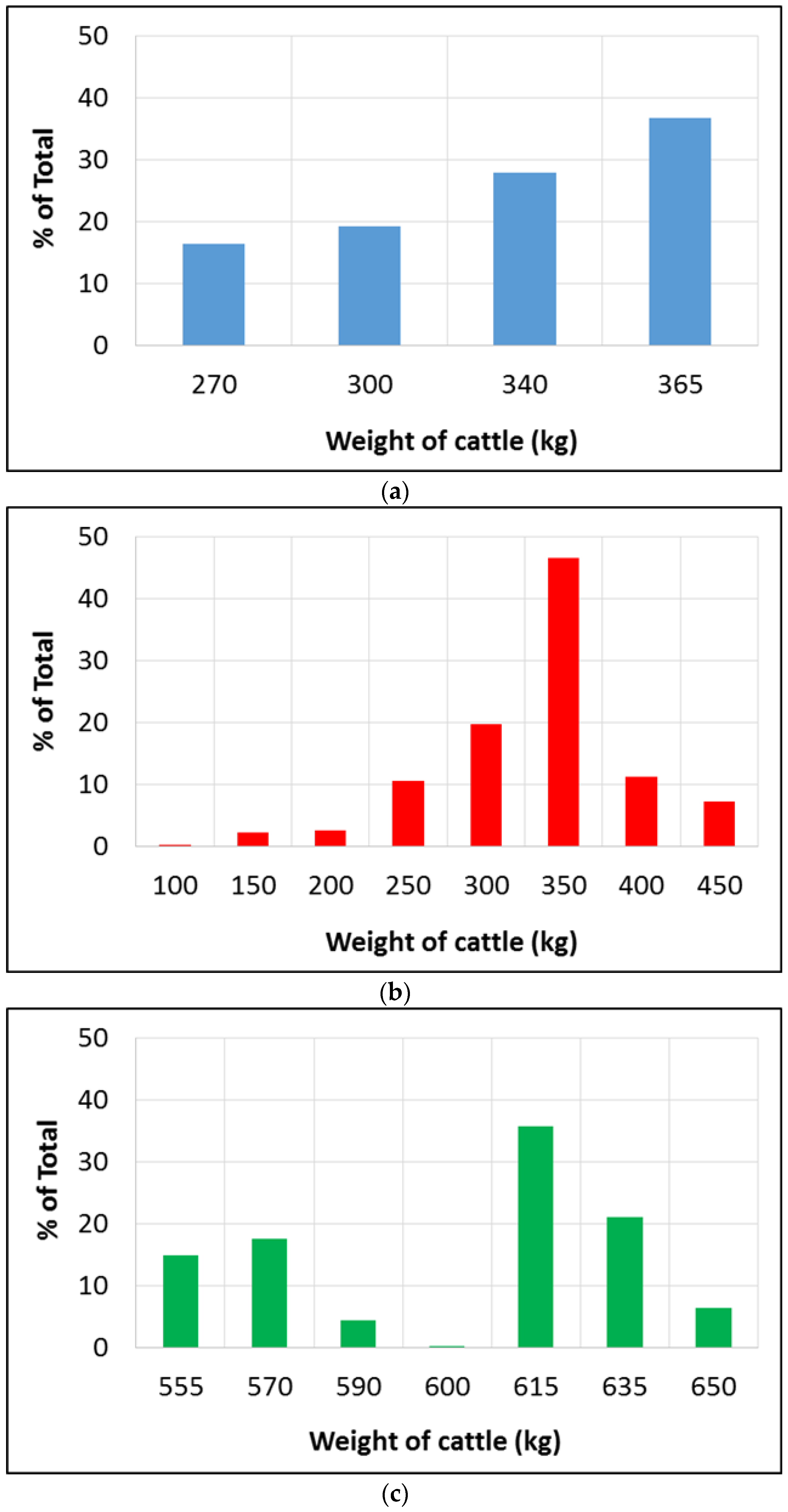
2.4.6. Distribution of Beef Cattle Getting Transported

Distribution for the purpose of this study refers to different weight categories of animals getting transported. For example, when feeder animals are transported to feedlots, they come in different sizes and weights. For meaningful interpretation of data, they can be grouped into a few categories. This will also help the user in entering the data into the computer model. This idea applies to finished cattle going to slaughterhouses and cattle transported to or from auction market. However, in the computer model developed as a part of this study, there is no limit on the number of weight categories of animals that can be entered by the user. The data on distribution of animals used in this study are shown in Figure 1. The distribution of animals (a) coming to feedlots; (b) going to (or) coming from auction; and (c) going to slaughterhouses are shown in Figure 1a–c, respectively. It should be noted that the distribution varies widely for the cattle transported to or from auction. The data is typically available on a weekly basis. It should be noted here that the data is highly variable, depending on time of the year, because of differences in calving season, management practices used for raising the animals, and also the climatic conditions. The data for Figure 1a is based on a typical week of cattle auction in Amarillo, TX. The distribution data on feeder cattle are based on USDA-NASS data [2,27] and the cattle going to slaughter are based on USDA data [25].

2.5. Allocation of Environmental Burden to Beef Byproducts

The beef cattle production LCA comes under a multiple output system (co-product systems). Therefore, as per the ISO 14046-1 standards [28], a three-step hierarchy should be followed on allocation of environmental burdens [29,30].
  • If possible, allocation should be avoided by expanding the system boundary.
  • If it is not possible to avoid allocation, the allocation problem must be solved by using physical relationships among functional units.
  • When physical relationships cannot be established, other relationships, including the economic value of the functional outputs, can be used.
In our beef LCA case, the environmental burden allocation cannot be avoided. The next step of solving the allocation problems comes up. The use of physical properties for establishing relationships include mass, energy content, volume, etc. Establishing physical relationships between beef and byproduct items could be an option to consider. However, it complicates the analysis because of lack of data availability, large difference in economic values of beef and by-products, and multiple industrial uses for many of the by-products. Therefore, the sensible option could be the use of the economic value of beef and the byproducts generated in the slaughterhouse, which was used in our analysis. Price data on live cattle and cattle by-products for the year 2013 are used in our analysis. The average purchase price of live cattle (average for the cattle sent to slaughter) is $2.78/kg (or $126.37 per cwt) [31] and the drop value (price of by-products generated) is $0.31/kg of live weight of animal (or $14.2 per cwt [32]. Considering the economic value, the proportion of environmental burden to be accounted for beef by-products is 0.31 × 100/2.79 = 11.15%.

3. Results

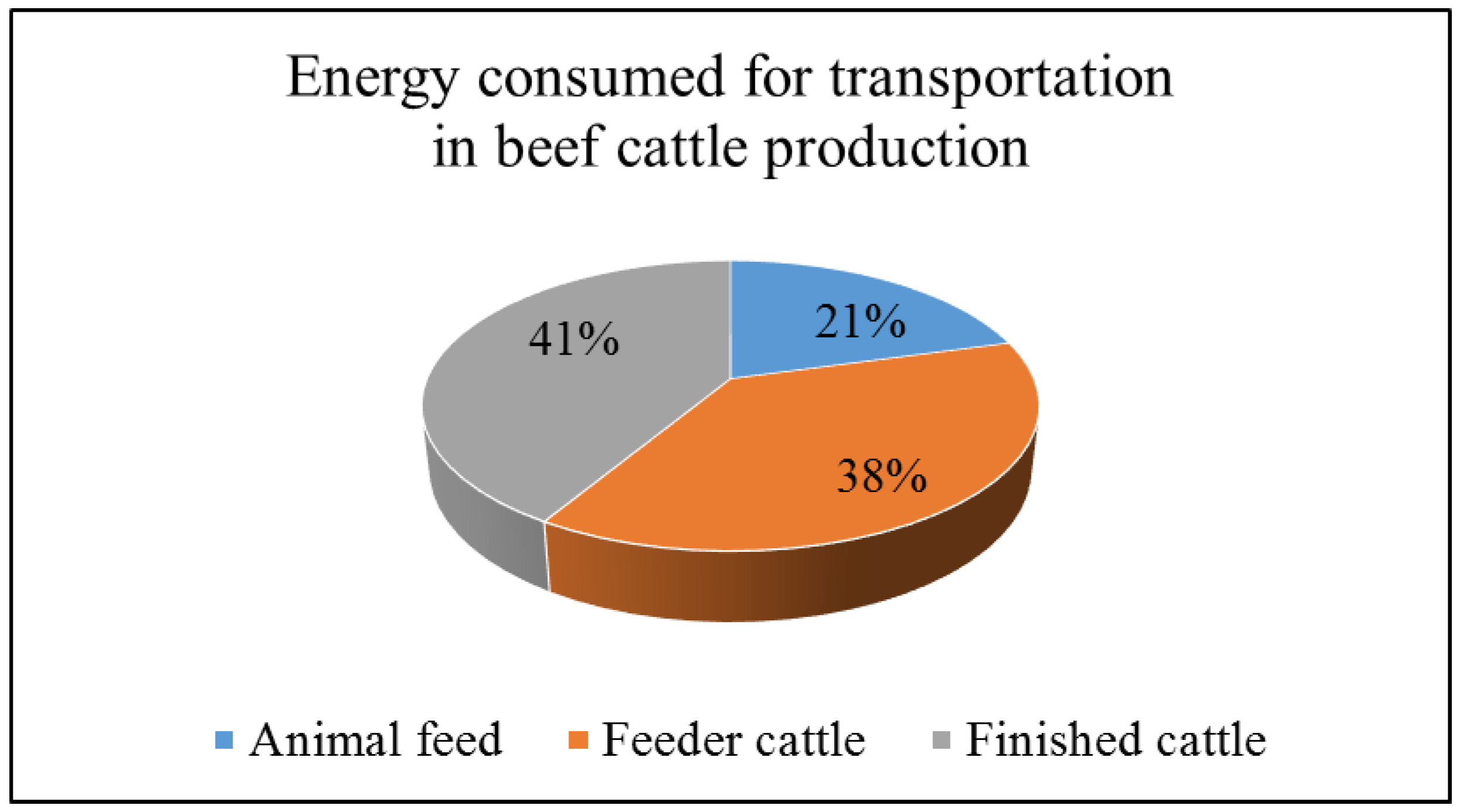
3.1. Energy Consumption of Transportation in Beef Cattle Production

Energy consumption results are presented per 1000 kg of beef and per animal basis. The summary of our analysis suggests that transporting finished cattle to slaughterhouses is the most energy-consuming transportation activity (8.1 L/1000 kg beef) (Table 3; Figure 2) for the study area. Bringing feeder cattle to feedlots shows a similar value (8 L/1000 kg beef) (Table 3). Although animal feed transportation involves many more truckloads, it shows moderate energy consumption rates. The energy consumption of transporting animal feed is about half of that used in transporting feeder cattle or finished cattle. Given a similar vehicle used for transporting animals and animal feed, distance appears to play a major role in deciding the energy consumption rate.

3.2. Greenhouse Gas Emissions for Transportation in Beef Cattle Production

Greenhouse gas emission results are presented per 1000 kg of beef and per animal basis. The summary of our analysis suggests that transporting finished cattle to slaughterhouses produces more greenhouse gases than transporting feeder cattle to feedlots and transporting animal feed (Table 4). The trend is similar to that of energy consumption. It is understandable, because greenhouse gas emissions have a direct relationship with energy consumption. Although animal feed transportation involves many more truckloads, it shows moderate GHG emission rates. The GHG emissions of transporting animal feed are about half that of transporting finished cattle and feeder cattle. This is because the distance of transportation is less in the case of animal feed transport.

3.3. Energy Consumption and Greenhouse Gas Emissions of Transporting Cattle to/from Auction

Energy consumption and greenhouse gas emission results from transporting cattle to and from auction is estimated on a per km basis using a gooseneck trailer and presented in Table 5. By knowing the distance transported in selling/buying cattle, a user can estimate the energy consumed and GHG emissions associated with this transport. Similar to animal transport and animal feed transport, the VMT for cattle going to auction and transported from auction are not available for the study region. Efforts are underway to estimate this. On a per km basis, cattle going to and coming from auction seems to be the least energy-consuming and greenhouse gas-emitting transportation operation (Table C1, Table C2, Table C3 and Table C4). This is probably because of the energy efficiency of the pickup trucks used in hauling the gooseneck trailers compared to other trailer-vehicle combinations.

4. Discussion

4.1. Sensitivity of Energy Consumption and Greenhouse Gas Emissions to Model Input Parameters

Sensitivity of model estimates of energy consumption and greenhouse gas emissions are quantified based on the changes in input parameters. Table 6 outlines those sensitivity results. A 10% change in market weight, or total headcount of cattle, or slaughter dressing proportion brings an 11% change in energy consumption and GHG emissions. The relationship is direct, meaning a 10% reduction in parameter value brings an 11% reduction in energy and GHG emissions. The slight non-linearity in output response is due to the approximation of animal weight to the nearest weight category (nearest 50 lb) and rounding of animal number fractions to the nearest whole number in the model. A 1% increase or decrease in cattle mortality rate results in a similar 1% increase or decrease in energy and GHG emission estimates. However, a 10% change in the weight of a single truckload results in a 5.6% change in energy and GHG emissions estimated by the animal feed transport model. Changes in vehicle type in the same category (e.g., 8a instead of 8b) results in a 34% change in resulting estimates. A change in fuel type does not change the energy consumption estimates. It, however, changes the resulting GHG emissions due to changes in energy content (or heat value) of fuel. A 10% change in distance transported results in a similar 10% change in energy and GHG emission estimates because the relationship between distance transported and the energy and GHG emissions is direct. A change with type of trailer within the same hitch category (e.g., different dimensions of pot belly trailer) results in 4.2% change in energy and GHG emission. On the other hand, if the user selects a totally different trailer, large changes (as much as 92%) are expected. In this case, selection of a smaller trailer increases the energy and GHG emission estimates and vice versa. Changes in energy consumption and GHG emission for changes in trailer sizes and vehicle class are presented to demonstrate the sensitivity of model output to input parameters. It should be noted that the sensitivity could be different for other changes (not described in Table 6) in input parameters. In the animal transport model, selection of one loading method over another does bring some differences in results. However, it is not to the extent of changes in vehicle type or trailer type.

4.2. Opportunities for Reducing Energy Consumption and Greenhouse Gas Emissions

As a part of this study, opportunities for reducing energy consumption and greenhouse gas emissions in transporting animals and animal feed were explored. Our analysis shows that, by simply switching the truck fuel from conventional diesel to a soy-based diesel, as much as 78% of GHG emissions can be reduced. Similar results were reported for soy-based biofuel by Huo et al. [34]. For the algae-based diesel, the reductions can be as much as 42% (Table 7), although the study by Batan et al. [35] points out higher values. The reductions are possible because of negative upstream greenhouse gas emissions. That is, in making biodiesel, plants are raised and oil is derived from plant-based material. It involves some greenhouse gas emissions. The CO2 captured by plants is much higher than the CO2 emissions produced in making the biodiesel [36]. Transporting animals may be unusual, or the present regulations may not permit animals in freight trains. However, a significant proportion of animal feed is transported through freight trains [37,38]. Our analysis shows that transporting animal feed through freight trains reduces energy consumption and greenhouse gas emissions by 53%. This is because of the high efficiency of trains in hauling large quantities of goods.

4.3. Additional Results

As a part of this study, energy consumption and greenhouse gas emissions are estimated on a per km basis for different truck–trailer combinations for fully-loaded trailers and trailers returning empty; this is presented in Appendix C (Table C1, Table C2, Table C3 and Table C4). This will help those involved in similar LCA studies outside our study region to have an estimate of energy consumption and greenhouse gas emissions by knowing the distance transported. In addition, these results can help those involved in transportation business to estimate fuel consumption in other parts of the USA.

5. Conclusions

A computer model was developed to quantify energy consumption and greenhouse gas emissions resulting from animal transport and animal feed transport. The model was applied to estimate data for the Life Cycle Analysis (LCA) of beef cattle production in the Southern Great Plains region. Cattle-related data to run the model was taken from the United States Department of Agriculture (USDA)–National Agricultural Statics Service’s (NASS) annual cattle slaughter data for Kansas and cattle on feed data provided by USDA–NASS for Kansas. In addition, a multi-agency transportation logistic study for meat-related industries in the Kansas region was used to get data on vehicle miles transported. Results were produced at the county level and summarized per animal and per 1000 kg of beef basis.
In the study region, feeder cattle are transported an average of 150 km (90 miles) to reach feedlots and get fed. Finished cattle travel a similar distance to reach slaughterhouses, whereas animal feed is transported for 22 km (13 miles) only, because most of the animal feed is going to be locally available. In terms of the annual number of truckloads, animal feed tops the list, with around 16,000, followed by transporting feeder cattle or finished cattle (around 4000). Our results on transportation in beef cattle production shows a total of 24 L of fossil fuel/1000 kg boneless beef (or 6 L per animal), excluding cattle transported to/from auction. On the other hand, the greenhouse gas emissions amount to 83 kg of CO2 equivalent/1000 kg of boneless beef (or 21 kg of CO2 equivalent per animal).
It appears that the majority of energy consumption and greenhouse gas emissions are associated with sending the finished cattle to slaughterhouses (41%), followed by bringing feeder cattle to feedlots (38%). Although the energy consumption and greenhouse gas emissions appear small on a per animal basis, about 10,000 animals are slaughtered for beef per day in the United States and, therefore, there are opportunities in transportation/beef cattle production to minimize the greenhouse gas emissions. Switching truck fuel from conventional to biodiesel could result in 42%–78% reductions in greenhouse gas emissions. Selection of the appropriate vehicle and trailer for transporting animals and animal feed appears to be critical to minimize energy consumption and greenhouse gas emissions. Definition of the correct vehicle type and trailer used to transport cattle or animal feed is necessary to obtain dependable results on energy consumption and greenhouse gas emissions from the model.

Acknowledgments

Funding provided by USDA to Project No. 2012-02355 through the National Institute for Food and Agriculture’s (NIFA) Agriculture and Food Research Initiative (AFRI), Regional Approaches for Adaptation to and Mitigation of Climate Variability and Change.

Author Contributions

Narayanan Kannan conceived and designed the experiments; Narayanan Kannan performed the experiments; Ali Saleh and Edward Osei analyzed the data; Narayanan Kannan wrote the paper.

Conflicts of Interest

The authors declare no conflict of interest.

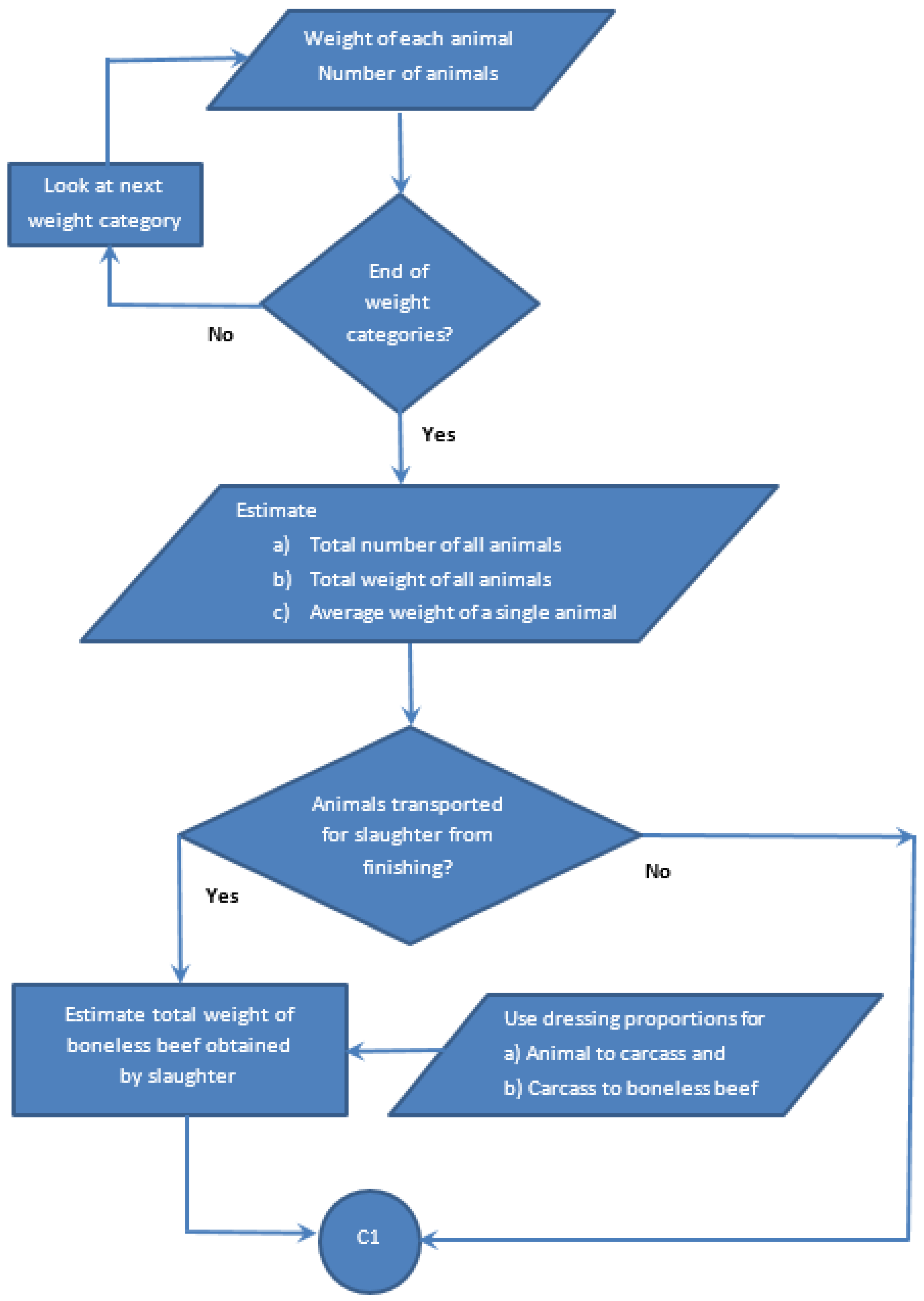
Appendix A. Sequence of Computations Used in the Model

The following is the sequence of computations involved in the animal transport model:
  • Read user-entered input parameters.
  • Estimate the total weight of boneless beef based on weight and number of animals transported in each category and slaughter dressing proportions.
  • Obtain trailer parameters from trailer database.
  • Estimate capacity of the trailer chosen and estimate total number of trips required to transport all the animals.
  • Read vehicle database and get parameters for the vehicle chosen.
  • Estimate total ton-miles using the trailer, vehicle parameters and total number of trips.
  • Estimate total fuel consumption and greenhouse gas emissions.
  • Express fuel consumption and greenhouse gas emissions per animal, and per kg of boneless beef basis.
The following is the sequence of computations involved in the animal feed transport model:
  • Read user-entered input parameters.
  • Estimate the total weight of boneless beef based on weight and number of animals fed and dressing proportions.
  • Read vehicle database and get parameters for the vehicle chosen.
  • Estimate total ton-miles for alfalfa, corn, sorghum, and supplements separately, using weight for each truckload, total number of truckloads, and vehicle parameters.
  • Estimate total fuel consumption and greenhouse gas emissions.
  • Express fuel consumption and greenhouse gas emissions per animal, and per kg of boneless beef basis.
Figure A1. Flow diagram of the animal transport model. GVWR is Gross Vehicle Weight Rating and C1, C2, and C3 are connectors used in the flow diagram.
Energies 09 00960 g003aEnergies 09 00960 g003b

Appendix B. Demonstration of Model Computations with an Example

Table B1. Vehicle database.
Vehicle ClassGVWR 1 (kg)Maximum Payload (kg)Fuel Use L/ton-kmTypical Vehicle 2
1c2719453169.7Cars only
1t2719680144.6Dodge Dakota, Chevrolet Colorado, GMC Canyon
2a3852113394.7Dodge Ram 1500, Chevrolet Silverado 1500, Ford F-150
2b4532167794.7Dodge Ram 2500, Chevrolet Silverado 2500, Ford F-250
36345237981.9Dodge Ram 3500, Ford F-350, GMC 3500
47251328658.5Ford F-450, GMC 4500, Dodge Ram 4500
58837394363.0GMC 5500, Dodge Ram 5500, Ford F-550
611,783521250.2Ford F-650, Chevrolet Kodiak, GMC TopKick
714,956838444.8Tractor-trailer, tow, refrigerated truck
8a36,25622,66021.4Straight truck, tow, dump, etc.
8b36,25624,47316.0Combination truck, tractor-trailer
T81,57654,3845.7Freight train-single car
1 GVWR: gross vehicle weight rating; 2 Typical vehicles include most commonly-used make models of pickup trucks. There are other make models of vehicles available in the market used by many for transporting animals.
Table B2. Trailer database.
TrailerLength (m)Width (m)GVWR (kg)Vehicle SuggestionType of Trailer
PB0116.22.624,9268bPot belly
PB0215.22.623,5668bPot belly
PB0314.62.422,6608aPot belly
PB0413.72.420,8478aPot belly
PB0511.62.115,4098aPot belly
GN0111.02.411,7666Gooseneck
GN029.82.410,2156Gooseneck
GN038.52.095176Gooseneck
GN048.52.095176Gooseneck
GN058.52.488545Gooseneck
GN069.12.173425Gooseneck
GN077.92.472514Gooseneck
GN087.32.472514Gooseneck
GN096.12.370254Gooseneck
GN105.52.167984Gooseneck
GN114.92.167984Gooseneck
GN127.32.167934Gooseneck
GN137.32.063453Gooseneck
GN147.32.063453Gooseneck
GN156.12.063453Gooseneck
GN164.92.054383Gooseneck
BP017.32.071067Bumper pull
BP027.32.070257Bumper pull
BP035.52.061187Bumper pull
BP044.92.045326Bumper pull
BP054.91.831725Bumper pull
BP064.32.047132bBumper pull
BP074.02.037662aBumper pull
Table B3. Distribution of cattle transported after finishing.
Weight of Finished Cattle in kg (lb)Number of Cattle
657 (1450)63
634 (1400)210
612 (1350)359
589 (1300)43
566 (1250)176
544 (1200)148
Table B4. User-defined input parameters to the model.
ParameterValueDetails
Distance transported in km (miles)216.8 (129.4)
Trailer used for moving finished cattlePB01Pot belly trailer
Truck used for hauling the trailer8bSemi-trailer truck
Fuel used in the truckDSLDiesel
Dressing 1: % of live animal wt. to carcass64
Dressing 2: % of carcass to boneless beef62
Boneless   beef = ( c = 1 n Weight   of   animal × Number   of   animals ) × Dressing 1 × Dressing 2
Boneless   beef = ( 657 × 63 ) + ( 634 × 210 ) + ( 612 × 359 ) + ( 589 × 43 ) + ( 566 × 176 ) + ( 544 × 148 ) × 64 × 62 100 × 100
Boneless   beef = 237 , 959   kg
Table B5. Estimated capacity of trailer under each weight category of animals (Calculated in advance and the model reads the information).
Animal Weight (kg)Proportion of Total Animals (%)Number of Animals in the Trailer
6576.336
63421.038
61235.938
5894.341
56617.642
54414.844
Average   capacity   of   trailer = c = 1 n Proportion × trailer   capacity   for   that   category
where n is number of categories of animals (different weight groups)
Average   capacity   of   trailer =   ( 6.3 × 36 ) + ( 21.0 × 38 ) + ( 35.9 × 38 ) + ( 4.3 × 41 ) + ( 17.6 × 42 ) + ( 14.8 × 44 ) 100 × 100 × 100 × 100 × 100 × 100
Average   capacity   of   trailer = 39.6   animals
Number   of   trips   needed = Total   number   of   animals   to   be   transported Average   capacity   of   trailer
Number   of   trips   needed = 999 39.6
Number   of   trips   needed = 25.2
Total   t k m = total   weight   ( truck + trailer + animals ) × number   of   trips × distance   transported
Weights of truck and trailer are taken from vehicle and trailer databases, respectively
total   weight   ( truck + trailer + animals ) = ( 8909 + 6500 + ( 39.6 × 600.3 ) )
total   weight   ( truck + trailer + animals ) = 39 , 181   kg
Total   t k m = 39 , 181 × 25.2 × 216.8 1000
Total   t k m = 214 , 363
Fuel   consumption   for   every   1000   t k m   is   16   L   ( from   vehicle   file )
Total   fuel   consumption = Total   t k m × Fuel   consumption   for   every   1000   t k m 1000
Total   fuel   consumption = 214 , 363 × 16.0 1000
Total   fuel   consumption = 3427.3   L   of   diesel
Energy   content   ( Low   Heat   Value   ( LHV ) ) of   diesel = 34 , 555.1 B T U L   ( taken   from   fuel   database )
Upstream   greenhouse   gas   emission   factor   for   diesel = 0.022   g   of   CO 2   equivalent / B T U   ( taken   from   the   fuel   database )
Tailpipe   greenhouse   gas   emission   factor   for   diesel = 0.08   g   of   CO 2   equivalent / B T U   ( taken   from   the   fuel   database )
Upstream / tailpipe   greenhouse   gas   emissions = Upstream / tailpipe   greenhouse   gas   emission   factor   for   the   fuel × Energy   content   of   the   fuel × Total   fuel   consumption
Total   greenhouse   gas   emissions = Upstream   greenhouse   gas   emissions + tailpipe   greenhouse   gas   emissions
Upstream   greenhouse   gas   emissions = 0.022 × 34 , 555.1 × 3427.3   grams   of   CO 2   equivalent
Upstream   greenhouse   gas   emissions = 2.6   tonnes   of   CO 2   equivalent
Upstream / tailpipe   greenhouse   gas   emissions   per   animal = Total   upstream / tailpipe   greenhouse   gas   emissions Total   number   of   animals
Upstream   greenhouse   gas   emissions = 2.6 × 1000 999   kg / animal
Upstream   greenhouse   gas   emissions = 2.6   kg / animal
Upstream / tailpipe   greenhouse   gas   emissions   per   kg   of   boneless   beef = Total   upstream / tailpipe   greenhouse   gas   emissions Total   boneless   beef   from   all   the   animals
Upstream   greenhouse   gas   emissions = 2.6 × 1000 × 1000 237 , 959 grams kg   boneless   beef
Upstream   greenhouse   emissions = 10.9   grams kg   of   boneless   beef
Tailpipe   greenhouse   gas   emissions = 0.08 × 34 , 555.1 × 3427.3   grams   of   CO 2   equivalent
Tailpipe   greenhouse   gas   emissions = 9.4   tonnes   of   CO 2   equivalent
Tailpipe   greenhouse   gas   emissions = 9.4 × 1000 999   kg / animal
Tailpipe   greenhouse   gas   emissions = 9.4   kg / animal
Tailpipe   greenhouse   gas   emissions = 9.4 × 1000 × 1000 237 , 959 grams kg   boneless   beef
Tailpipe   greenhouse   emissions = 39.6   grams kg   of   boneless   beef
Total   greenhouse   gas   emissions   per   animal   = 2.6 + 9.4 = 12   kg / animal
Total   greenhouse   gas   emissions   per   kg   of   beef = 10.9 + 39.6 = 50.5   grams   of   CO 2   equivalent   per   kg   of   boneless   beef
Table B6. Weight and number of truckloads of animal feed transported.
Animal FeedNumber of TruckloadsWeight of a Single Truckload (t)
Corn10,97521.8
Grain sorghum745020.9
Alfalfa474411.8
Supplements58022.7
Table B7. User-defined input to the animal feed transport model.
ParameterValueDetails
Market weight of cattle in kg (lb)604.1 (1333)Average finished weight in feedlot
Total number of animals fed67,800Real data for example computation
Mortality rate in feedlot (%)1.5Dead animals not included in calculations
Dressing 1 (%) 64Dressing of live animal to carcass
Dressing 2 (%)62Dressing of carcass to boneless beef
Distance transported (km)24.8One-way distance from origin to feedlot
Vehicle used for transport8bMore details in vehicle database
Fuel used in vehicleDSLFuel used in the vehicle is diesel
Number   of   animals   dead = Mortality   rate   ( % ) × Total   number   of   animals   fed 100
Number   of   animals   dead = 1.5 × 67 , 800 100 = 1017
Number   of   animals   living = Total   number   of   animals   fed total   number   of   animals   dead
Number   of   animals   living = 67 , 800 1017 = 66 , 783
Boneless   beef = Number   of   animals   living × weight   of   each   animal × dressing   1 × dressing   2 100 × 100
Boneless   beef = 66 , 783 × 604.1 × 64 × 62 100 × 100
Boneless   beef = 16 , 008 , 345   kg
Total   t k m = Weight   of   a   sin gle   truckload × total   number   of   truckloads   transported × distance   transported
Example calculations for transporting grain sorghum to feeder cattle
For   Sorghum ,   Total   t k m = 20.9 × 7450 × 24.8 = 3 , 861 , 484
Total   fuel   consumption = 3 , 861 , 484 × 16 1000 = 61 ,   784   L   of   diesel
Total   fuel   consumption = 61 , 784 66 , 783 = 0.92   L / animal
Total   fuel   consumption = 61 , 694 × 1000 16 , 008 , 345 = 3.85 mL kg   of   boneless   beef
Price   of   one   beef   animal   is   $ 2.78   per   kg   of   live   weight   ( USDA AMS )
Price of byproducts obtained from one beef animal is $0.31 per kg of live weight [32]
Proportion   of   environmental   burden   to   beef   by - products = Price   of   beef   by products Price   of   live   animal × 100 = 0.31 2.78 × 100
Proportion   of   environmental   burden   to   beef   by products = 11.15 %

Appendix C. Additional Results on Energy Consumption and Greenhouse Gas Emissions for Various Truck-Trailer Combinations on a per km Basis

Table C1. Energy consumption and greenhouse gas emissions for cattle feed transport.
Animal feedFuel Consumption (L/km)Greenhouse Gas Emissions (kg of CO2 Equivalent/km)
Fully-LoadedEmptyFully-LoadedEmpty
Alfalfa0.650.362.271.29
Corn0.890.363.11.29
Grain sorghum0.860.363.031.29
Supplements0.910.363.181.29
Average0.830.362.891.29
Min–Max0.65–0.91 2.27–3.18
Table C2. Energy consumption and greenhouse gas emissions for cattle transport to auction.
Trailer TypeCompatible VehicleFuel Consumption (L/km)Greenhouse Gas Emissions (kg of CO2 Equivalent/km)
Fully-LoadedEmptyFully-LoadedEmpty
GN01–GN0460.60–0.680.291.72–2.000.85
GN05–GN0650.55–0.630.281.61–1.850.80
GN07–GN1240.44–0.500.201.26–1.450.60
GN13–GN1630.56–0.600.281.64–1.740.84
Average 0.550.261.620.75
95% CI 0.52–0.590.24–0.281.51–1.720.69–0.80
Min–Max 0.44–0.680.20–0.291.26–2.000.60–0.85
Table C3. Energy consumption and greenhouse gas emissions for cattle transport to feedlot.
Trailer TypeCompatible VehicleFuel Consumption (L/km)Greenhouse Gas Emissions (kg of CO2 Equivalent/km)
Fully-LoadedEmptyFully-LoadedEmpty
PB01–PB028b0.53–0.560.221.87–1.970.76
PB03–PB058a0.720.292.511.02
Average 0.650.262.280.92
95% CI 0.57–0.730.23–0.301.99–2.560.80–1.04
Min–Max 0.53–0.720.22–0.291.87–2.510.76–1.02
Table C4. Energy consumption and greenhouse gas emissions for cattle transport from feedlot to slaughterhouse.
Trailer TypeCompatible VehicleFuel Consumption (L/km)Greenhouse Gas Emissions (kg of CO2 Equivalent/km)
Fully-LoadedEmptyFully-LoadedEmpty
PB01–PB028b0.52–0.560.221.83–1.950.76
PB03–PB058a0.700.292.461.02
Average 0.640.262.230.92
95% CI 0.56–0.720.23–0.301.95–2.510.80–1.04
Min–Max 0.52–0.700.22–0.291.83–2.460.76–1.02

References

  1. USDA (United States Department of Agriculture)-NASS (National Agricultural Statistics Service). Field Crops Usual Planting and Harvesting Dates; Agricultural Handbook Number 628; USDA-NASS: Washington, DC, USA, 2010.
  2. USDA (United States Department of Agriculture)-NASS (National Agricultural Statistics Service). Cattle Inventory Report; Agricultural Statistics Board: Washington, DC, USA, 2014.
  3. McBride, W.D.; Mathews, K., Jr. The Diverse Structure and Organization of U.S. Beef Cow-Calf Farms; EIB-73; U.S. Department of Agriculture, Economic Research Service-United States Department of Agriculture: Washington, DC, USA, 2011.
  4. Great Plains Grazing. Available online: http://www.greatplainsgrazing.org/ (accessed on 24 August 2016).
  5. Klopfenstein, T. North American Beef Industry. In Proceedings of the Beef Methane Conference, Lincoln, NE, USA, 11–12 May 2016.
  6. Argonne National Laboratory. 2012 GREET Website. Available online: http://greet.es.anl.gov (accessed on 23 August 2016).
  7. GREET Publications of the GREET Model Development and Applications. Available online: https://greet.es.anl.gov/fleet_footprint_calculator (accessed on 24 August 2016).
  8. Elgowainy, A.; Han, J.; Poch, L.; Wang, M.; Vyas, A.; Mahalik, M.; Rousseau, A. Well-to-Wheels Analysis of Energy Use and Greenhouse Gas Emissions of Plug-In Hybrid Electric Vehicles; U.S. Department of Energy, Argonne National Lab: Chicago, IL, USA, 2010.
  9. Tiax LLC. Full Fuel Cycle Assessment: Well-to-Wheels Energy Inputs, Emissions, and Water Impacts; Report Prepared for California Energy Commission, CEC-600-2007-004-F; Tiax LLC.: Lexington, MA, USA, 2007. [Google Scholar]
  10. Bai, Y.; Oslund, P.; Mulinazzi, T.; Tamara, S.; Liu, C.; Barnaby, M.M.; Atkins, C.E. Transportation Logistics and Economics of the Processed Meat and Related Industries in Southwest Kansas; Final Report from a co-Operative Transportation Research Program with Kansas State University; KU-06-3; University of Kansas and Kansas Department of Transportation: Lawrence, KS, USA, 2007. [Google Scholar]
  11. Grandin, T. Livestock Trucking Guide; Livestock Conservation Institute: Bowling Green, KY, USA, 1981. [Google Scholar]
  12. Grandin, T. Recommended Animal Handling Guidelines & Audit Guide: A Systematic Approach to Animal Welfare; American Meat Institute Foundation: Washington, DC, USA, 2010. [Google Scholar]
  13. Brown, A.; Nae, D.A.; Bezdek, R.; Clark, N.; Corsi, T.M.; Foster, D.; Fruechte, R.D.; Hu, G.; Johnson, J.H.; Kodjak, D.; et al. Technologies and Approaches to Reducing the Fuel Consumption of Medium and Heavy Duty Vehicles; National Research Council of the National Academies, National Academic Press: Washington, DC, USA, 2010. [Google Scholar]
  14. Ford. RV and Trailer Towing Guide, RV-VER9480–0914. 2015. Available online: http://www.fleet.ford.com/resources/ford/general/pdf/towingguides/Ford_Linc_16RVTTgde_r3_Nov12.pdf (accessed on 23 August 2016).
  15. Fuel Efficient Freight Trains? Available online: http://www.factcheck.org/2008/07/fuel-efficient-freight-trains/ (accessed on 6 July 2016).
  16. Alternative Fuels and Advanced Vehicles. Available online: http://www.afdc.energy.gov/fuels/index.html (accessed on 6 July 2016).
  17. National Cattlemen’s Beef Association. Master Cattle Transporter Guide. Beef Quality Assurance Program; National Cattlemen’s Beef Association: Centennial, CO, USA, 2007. [Google Scholar]
  18. Whiting, T.L. Comparison of minimum space allowance standards for transportation of cattle by road from 8 authorities. Can. Vet. J. 2000, 41, 855–860. [Google Scholar] [PubMed]
  19. National Cattlemen’s Beef Association. Stock Trailer Transportation of Cattle. Beef Quality Assurance Program; National Cattlemen’s Beef Association: Centennial, CO, USA, 2007. [Google Scholar]
  20. ILAR Transportation Guide. Guidelines for the Humane Transportation of Research Animals; National Academies Press: Washington, DC, USA, 2006. [Google Scholar]
  21. Schwartzkopf-Genswein, F.L.; Dadgar, S.; Shand, P.; Gonzalez, L.A.; Crowe, T.G. Road transport of cattle, swine and poultry in North America and its impact on animal welfare, carcass and meat quality: A review. Meat Sci. 2012, 92, 227–243. [Google Scholar] [CrossRef] [PubMed]
  22. Cole, N.A.; Brown, M.S.; Varel, V.H. Beef Cattle: Manure Management in Encyclopedia of Animal Science, 2nd ed.; Ullrey, D.E., Baer, C.K., Pond, W.G., Eds.; CRC Press: Boca Raton, FL, USA, 2011. [Google Scholar]
  23. Kelly, A.P.; Janzen, E.D. A review of morbidity and mortality rates and disease occurrence in North American feedlots. Can. Vet. J. 1986, 27, 496–500. [Google Scholar] [PubMed]
  24. Beckett, J.L.; Oltjen, J.W. Estimation of the water requirement for beef production in the United States. J. Anim. Sci. 1993, 71, 818–826. [Google Scholar] [PubMed]
  25. USDA. Kansas Yearly Weighted Average Cattle Report (2015); USDA Livestock, Poultry & Grain Market News Division: St. Joseph, MO, USA. Available online: www.ams.usda.gov/market-news/livestock-poultry-grain (accessed on 21 July 2016).
  26. Cole, A.; (Conservation and Production Research Laboratory, United States Department of Agriculture-Agricultural Research Service, Bushland, TX, USA). Personal communication, 2016.
  27. USDA (United States Department of Agriculture)-NASS (National Agricultural Statistics Service). Cattle on Feed (2015); Collection of Monthly Cattle on Feed Report for the Year 2015; USDA-NASS: Washington, DC, USA, 2015.
  28. ISO 14061-1:2006. Greenhouse Gases Part 1: Specification with Guidance at the Organization Level for Quantification and Reporting of Greenhouse Gas Emission and Removals; International Organization for Standardization: Geneva, Switzerland, 2006. [Google Scholar]
  29. Azapagic, A.; Clift, R. Allocation of environmental burdens in co-product systems: Product-related burdens (Part 1). Int. J. Life Cycle Assess. 1999, 4, 357–369. [Google Scholar] [CrossRef]
  30. Azapagic, A.; Clift, R. Allocation of environmental burdens in co-product systems: Process and product-related burdens (Part 2). Int. J. Life Cycle Assess. 1999, 5, 31–36. [Google Scholar] [CrossRef]
  31. LM_CT170. Available online: https://www.ams.usda.gov/mnreports/lm_ct170.txt (accessed on 24 August 2016).
  32. United States Department of Agriculture (USDA). 2013 Annual Meat Trade Review; United States Department of Agriculture-Agricultural Marketing Service, Livestock and Grain Market News Service: Des Moines, IA, USA, 2013.
  33. Vehicle Weight Classes & Categories. Available online: http://www.afdc.energy.gov/data/10380 (accessed on 24 August 2016).
  34. Huo, H.; Wang, M.; Bloyd, C.; Putsche, V. Life-cycle assessment of energy use and greenhouse gas emissions of soybean-derived biodiesel and renewable fuels. Environ. Sci. Technol. 2009, 43, 750–756. [Google Scholar] [CrossRef] [PubMed]
  35. Batan, L.; Quinn, J.; Willson, B.; Bradley, T. Net energy and greenhouse gas emission evaluation of biodiesel derived from microalgae. Environ. Sci. Technol. 2010, 44, 7979–7980. [Google Scholar] [CrossRef] [PubMed]
  36. Biodiesel Vehicle Emissions. Available online: http://www.afdc.energy.gov/vehicles/diesels_emissions.html (accessed on 23 August 2016).
  37. Sparger, A.; Nick, M. Transportation of U.S. Grains: A Modal Share Analysis; USDA Agricultural Marketing Service. June 2015. Available online: https://www.ams.usda.gov/services/transportation-analysis/modal (accessed on 21 July 2016). [Google Scholar]
  38. Denicoff, M.R.; Prater, M.E.; Bahizi, P. Wheat Transportation Profile; USDA Agricultural Marketing Service. November 2014. Available online: https://www.ams.usda.gov/sites/default/files/media/Wheat%20Transportation%20Profile.pdf (accessed on 23 August 2016). [Google Scholar]
Figure 1. Distribution of animals transported: (a) Feeder cattle; (b) Cattle auction; and (c) Finished cattle.
Energies 09 00960 g001
Figure 2. Energy (diesel) consumed for transportation in beef cattle production.
Energies 09 00960 g002
Table 1. Annual average truckloads of animal feed, feeder cattle, and finished animals transported [10].
CategoryAnnual Average Truckloads
Number of Truckloads95% Confidence LimitsRange (Minimum to Maximum)
Feeder cattle to feed-yards42753358–519221–7936
Animal feed to feed-yards15,8869239–22,534157–58,445
Finished cattle to slaughter35952091–510036–13,228
Total truckloads23,75612,584–30,693214–79,609
Table 2. Annual average vehicle miles per truck load transported for animal feed, feeder cattle, and finished animals to slaughter.
CategoryVehicle Miles Transported (VMT)
km95% Confidence LimitsRange (Minimum to Maximum)
Feeder cattle to feed-yards149.7128.0–171.121.4–257.9
Animal feed to feed-yards22.320.8–23.815.6–30.7
Finished cattle to slaughter153.7138.3–169.183.1–230.3
Total vehicle miles325.6304.4–352.0240.5–461.7
Table 3. Energy consumption in beef cattle production: transporting animal feed, feeder cattle, and finished animals to slaughter.
CategoryDiesel Used in Transportation
L/1000 kg Beef95% Confidence LimitsL/Animal95% Confidence Limits
Feeder cattle to feed-yards8.07.0–9.02.01.7–2.2
Animal feed to feed-yards4.13.7–4.61.00.9–1.1
Finished cattle to slaughter8.17.0–9.22.01.7–2.3
Total20.218.8–21.75.04.7–5.4
Table 4. Greenhouse gas emissions in beef cattle production: transporting animal feed, feeder cattle, and finished animals to slaughter.
CategoryGreenhouse Gas Emissions: CO2 Equivalent
kg/1000 kg Beef95% Confidence Limitskg/Animal95% Confidence Limits
Feeder cattle to feed-yards28.124.8–31.57.06.2–7.8
Animal feed to feed-yards15.314.3–16.33.83.6–4.1
Finished cattle to slaughter29.025.0–32.97.26.2–8.2
Total72.465.8–76.118.016.4–19.0
Table 5. Energy consumption and greenhouse gas emissions for cattle transport to/from auction.
Trailer TypesCompatible Vehicle Class (GVWR kg)Energy Consumption (L/km)Greenhouse Gas Emission (kg of CO2 Equivalent/km)
GN01–GN046 (11,783)0.60–0.681.72–2.00
GN05–GN065 (8837)0.55–0.631.61–1.85
GN07–GN124 (7251)0.44–0.501.26–1.45
GN13–GN163 (6345)0.56–0.601.64–1.74
Average 0.551.62
95% confidence 0.52–0.591.51–1.72
Min–max 0.44–0.681.26–2.00
Note: GN is a gooseneck trailer. All the above listed vehicle classes come under medium-duty truck under U.S. Federal Highway Administration classification system [33].
Table 6. Sensitivity of model estimates of energy consumption and greenhouse gas emissions from the animal feed and animal transport models for different changes in input parameters.
Input ParameterChange% Change in
EnergyGHG Emission
Market weight/Number of cattle, dressing10%11.111.1
Mortality rate in feedlot±1%1.01.0
Quantity/Weight of single truckload of animal feed10%5.65.6
Vehicle selected for transporting8a for 8b33.833.9
Fuel type used in the vehicle (default diesel)Gasoline0.017.0
Distance transported10%10.010.1
Trailer used for transporting animalsPB03 for PB014.24.2
Trailer used for transporting animalsGN01 1 for PB0191.891.8
Changing loading method (default arranged loading)Thoughtless dumping−1.8−1.8
Changing loading method (default arranged loading)Loading pressure equation7.47.4
1 GN01 is a different category trailer and much smaller than PB01.
Table 7. Opportunities for reducing energy and greenhouse gas emissions.
Input ParameterDecrease (%) in
EnergyGHG Emission
Soy-based diesel as fuel instead of conventional diesel0.078.1
Algae-based diesel as fuel instead of conventional diesel0.042.5
Transporting using freight train instead of truck52.752.6

