Mapping the Geothermal System Using AMT and MT in the Mapamyum (QP) Field, Lake Manasarovar, Southwestern Tibet

Abstract

Southwestern Tibet plays a crucial role in the protection of the ecological environment and biodiversity of Southern Asia but lacks energy in terms of both power and fuel. The widely distributed geothermal resources in this region could be considered as potential alternative sources of power and heat. However, most of the known geothermal fields in Southwestern Tibet are poorly prospected and currently almost no geothermal energy is exploited. Here we present a case study mapping the Mapamyum (QP) geothermal field of Southwestern Tibet using audio magnetotellurics (AMT) and magnetotellurics (MT) methods. AMT in the frequency range 11.5–11,500 Hz was used to map the upper part of this geothermal reservoir to a depth of 1000 m, and MT in the frequency range 0.001–320 Hz was used to map the heat source, thermal fluid path, and lower part of the geothermal reservoir to a depth greater than 1000 m. Data from 1300 MT and 680 AMT stations were acquired around the geothermal field. Bostick conversion with electromagnetic array profiling (EMAP) filtering and nonlinear conjugate gradient inversion (NLCGI) was used for data inversion. The AMT and MT results presented here elucidate the geoelectric structure of the QP geothermal field, and provide a background for understanding the reservoir, the thermal fluid path, and the heat source of the geothermal system. We identified a low resistivity anomaly characterized by resistivity in the range of 1–8 Ω∙m at a depth greater than 7 km. This feature was interpreted as a potential reflection of the partially melted magma in the upper crust, which might correlate to mantle upwelling along the Karakorum fault. It is likely that the magma is the heat source of the QP geothermal system, and potentially provides new geophysical evidence to understand the occurrence of the partially melted magmas in the upper crust in Southwestern Tibet.

1. Introduction

Renewable energy is attracting attention globally as the overuse of fossil fuels challenges our abilities to limit cumulative carbon emissions in the future [1]. Geothermal energy, a source of renewable energy naturally present inside the Earth’s crust, could be extracted, potentially, at costs competitive to other forms of energy at some point in the future [2,3], and the utilization of geothermal energy has rapidly increased over the last three decades [4]. Southwestern Tibet, one of the most environmentally pristine places in the world, plays a crucial role in the protection of ecology and biodiversity in South Asia and globally. However, although this region has been considered as a source for renewable, clean energy, the development of solar and wind power is not feasible because of interrupted supply. Geothermal regions are widely distributed in Southwestern Tibet but, because they have been poorly prospected, their utilization remains uncommon. In order to map the geothermal system, a comprehensive geophysical prospecting has been conducted in the QP geothermal field in Southwestern Tibet.

Geothermal energy has, so far, been utilized in more than 100 countries or regions, and uptake has increased by around 12 percent each year as deep buried geothermal reservoirs (with a depth of 1000–5000 m) have become targets for prospecting [5]. It has become more and more challenging to use traditional geological methods to identify deeply buried geothermal reservoirs as these rely on the availability of point measurements, including hot spots, and water sample analysis [6]. Geophysical detection and monitoring of reservoirs with several kilometers in depth is key to exploration of geothermal energy [7]. Electromagnetic (EM) methods have been widely applied in geothermal exploration as resistivity is very sensitive to the presence of brine [7], and the electrical conductivity of the subsurface is known to be a crucial parameter for the characterization of geothermal settings [8]. Geothermal systems generally have higher conductivity than their host rocks, because of alterations to clay minerals due to hydrothermal processes, and the fact that faults where the system occurs and geothermal fluids all act as electrical conductors. This makes geothermal systems ideal targets for the application of EM methods [8], with two such approaches based on natural sources, audio magnetotellurics (AMT) and magnetotellurics (MT), widely applied in volcanic areas for structural investigations, geothermal evaluation, and the determination of hydrothermal circulation [9]. The MT and AMT methods use the natural EM field around the Earth as a source and provides useful information about lateral and vertical resistivity variations in the subsurface. MT has a depth of exploration ranging from tens of meters to more than 10 km [10]. In contrast, because AMT has a frequency range of 11.5–11,500 Hz, it has a relative shallow exploration depth and is commonly applied for evaluating shallow geothermal reservoirs with a depth less than 1000 m.

The QP geothermal field, also known as the Mapamyum geothermal field, is located on the Himalayan-Tibetan orogen. The Himalayas are a classic example of an orogenic system caused by a continent-continent collision, while their relatively young age and spectacular exposure make this region ideal for studying the diverse geological processes related to mountain-building that can then be applied to other areas that were formed in a similar way [11]. In addition, neotectonic activity in Southwestern Tibet, mostly related to the northerly movement of the Indian Plate towards the Eurasian Plate, means that all kinds of geothermal features (including geysers, boiling springs, hot springs, and mud springs) occur in this region. However, most geothermal sites in Southwestern Tibet remain poorly understood, we present AMT and MT exploration results for the QP geothermal system and discuss their implications.

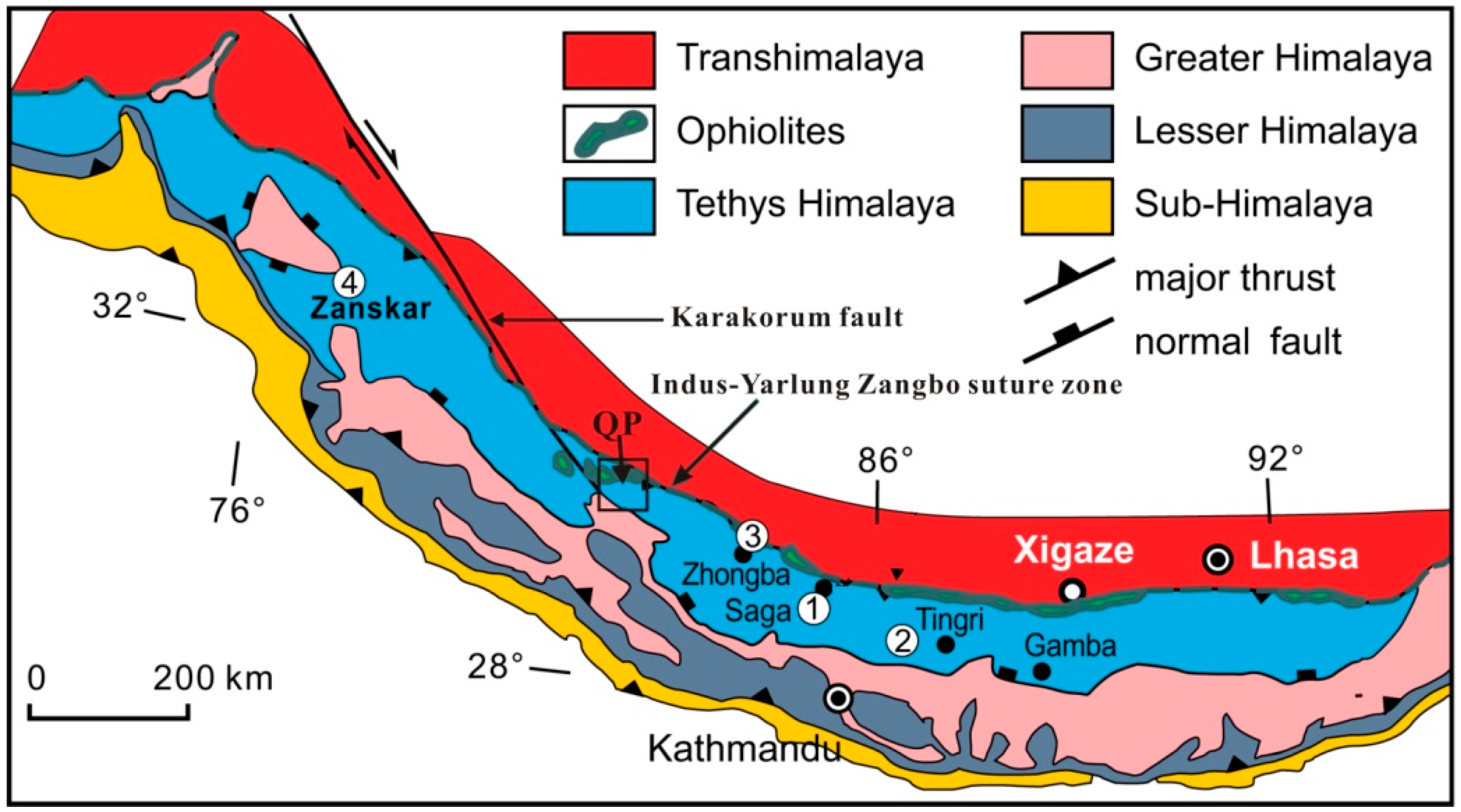
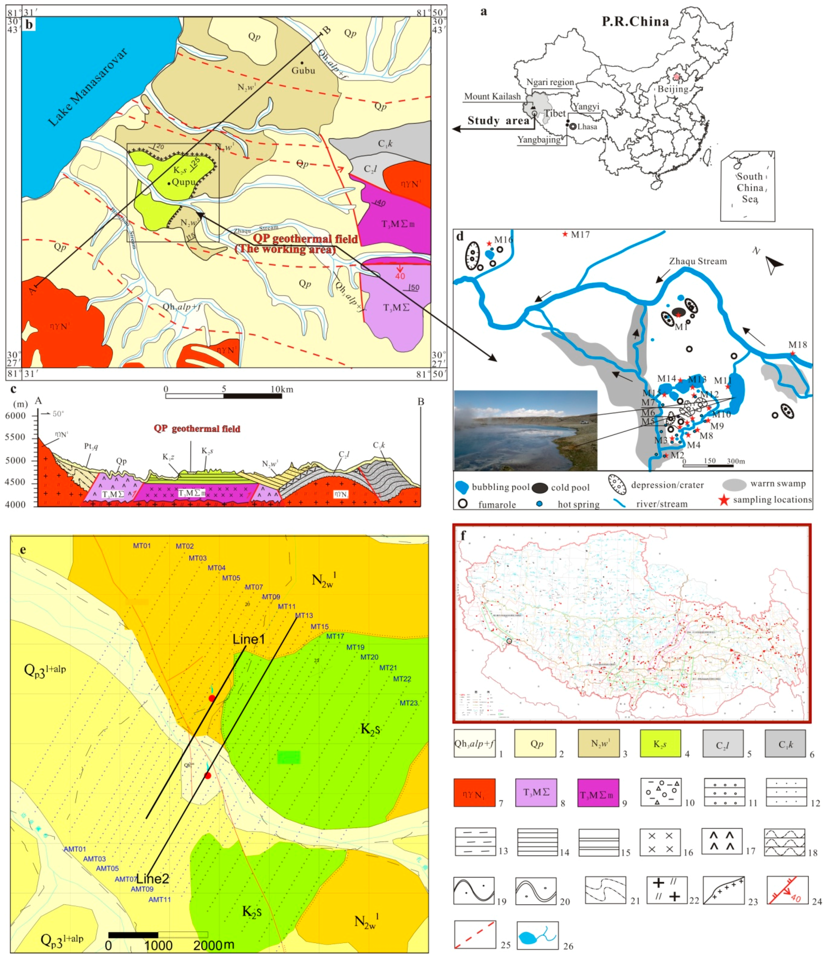
2. Background and Geological Setting

The QP geothermal field is located on the complex structural unit between the eastern portion of the Karakorum fault and the western portion of the Indus-Yarlung Zangbo suture zone (Figure 1). The Karakorum fault, which has a trend line of more than 1000 km, is one of the most morphologically prominent structures in the western region of the Himalayan-Tibetan orogen [12]. The Indus-Yarlung Zangbo suture zone, which has a trend line of more than 2000 km from west to east, separates Eurasia to the north from the Indian continent to the south [13,14]. Continent-continent collision between the Eurasian and Indian plates and interactions within Himalayan-Tibetan orogen were initiated 59 ± 1 Ma ago [15] and continue to the present day. As a result, abundant geothermal resources are distributed in Tibet, considered the eastern region of the Mediterranean-Himalayan geothermal zone. For example, more than 600 hot springs have been identified in Tibet (Figure 2f), more than 100 of which have a temperature higher than 100 °C; the QP geothermal field is one such example located in the western region of the Himalayan geothermal zone [16].

Most of the study area for this research is covered by lake sediments and Quaternary hot spring deposits (Figure 2). Strata that outcrop in this area include the Sangdanling Group of upper Cretaceous rocks (K₂s) and the Woma Formation, part of the Neogene Kailas Group (N₂w). The Upper Cretaceous (K₂s) units comprise interbedded sandstones, shales, and mudstones, with gravel-bearing sandstones at their base. Major components of these gravels are igneous rocks, while the Woma Formation (N₂w) comprises of grey gravels, yellow sandstones, and yellowish-gray mudstones in increasing abundance. Major components of these gravels are, again, igneous rocks, but quartz conglomerates are also found, rarely; the average particle size is 0.3–3 cm, but the largest clasts can reach up to 6 cm. The QP geothermal field is one of the most famous hot spots in Southwestern Tibet, one of more than five developed in an area of about 100 km². The geothermal characteristics of the QP field include geothermal explosions, mud pots, boiling, hot, and thermal springs. The most recent geothermal explosion in the QP field was an eruption in 1977, when a geothermal lake was formed. Calcareous deposits associated with hydrothermal springs cover more than 2 km², and the largest sinter cone in this region has height of more than 50 m. Wang et al. [17] provided the results of a detailed geochemical investigation on the hydrothermal waters of this field and discussed the ion origin and phase equilibria of minerals, the mixing of thermal and cold waters, the geothermal reservoir temperature, and the origin of carrier CO₂ in the hydrothermal water. The hydrothermal water in the QP geothermal field is a Na-HCO₃ type, containing a large amount of CO₂-rich gases of magmatic and metamorphic sources; the temperature of this geothermal reservoir is approximately 220 °C [17].

3. Methods, Data Acquisition, and Processing

AMT and MT are natural or passive source electromagnetic methods that utilize natural magnetotelluric fields in the audio (for AMT, 10 Hz–10 kHz) or normal frequency bands (for MT, 0.001–1000 Hz) to investigate the electrical conductivity structure of the Earth [18]. The MT method was first formulated by Tikhonov [19] and Cagniard [20,21]. Natural AMT and MT fields above about 1 Hz are generated by thunderstorms, as energy discharged by lightning emits EM fields that can propagate great distances. At frequencies below 1 Hz, the bulk of an EM signal is due to current systems in the magnetosphere created by solar activity [18,22]. AMT and MT fields at the surface of the Earth behave like plane waves, while basic theory, field operation, and data processing are almost the same for both methods with the exception of the frequency band and data acquisition duration. Specifically, AMT and MT methods measure orthogonal electric (E) and magnetic (H or B) fields and generate frequency-based impedance results in response to the distribution of electrical conductivity in the subsurface. From these data, amplitude of apparent resistivity, phase of impedance, and the directional relationships between electric and magnetic fields at the surface can be generated by the commercial package of SSMT2000 and MTEDITOR from Phoenix Geophysics (Toronto, ON, Canada) [18,22].

We carried out an EM survey over a 60 km² area around the QP geothermal field (Figure 2). Over the whole working area, 1300 MT stations were used comprising two kinds of grids. Of these, the first type had a line separation of 1000 m and a station separation of 200 m (1000 m × 200 m) arranged around the outer rim, while the other type were arrayed in a 200 m × 100 m configuration in the central region of the study area. Similarly, 680 AMT stations with a grid spacing of 200 m × 100 m were also arrayed in the central portion (Figure 2). The complete survey took three months, from May to July, 2013. More than 20 sets of PMT-1 (a kind of AMT receiver designed and produced by Champion Geophysics, Changsha, China) multi-channel AMT receivers and 40 sets of PMT-2 (Champion Geophysics) multi-channel MT receivers were used for AMT and MT data acquisition. Data from two orthogonal magnetic fields and two orthogonal electric fields were recorded by the receivers, while four lead-lead chloride (Pbcl-Pb) electrodes (for electric fields in two orthogonal directions, Ex and Ey) and a pair of coils (for magnetic fields in two orthogonal directions, Hx and Hy) were used to measure the orthogonal components of the electromagnetic field at each station (See [23] for a detailed description of the AMT field layout). AMT acquisition frequencies were in the range of 11.2–10,040 Hz, the data acquisition duration was greater than 30 min, while frequencies for MT were in the range of 0.001–320 Hz with a duration of more than 8 h. AMT acquired data only during the daytime, while MT works day and night. There are very few artificial noises in the working area, allowing high quality data of both AMT and MT features. Eighty-nine percent of MT data and 92 percent of AMT data were characterized by quality of “first grade” according to the Industry Standard of the China Geological Survey. The electrode lengths for electric field recordings is 20 to 40 m for AMT and 50 to 100 m for MT. Some data were acquired using single-station mode, more than half of the stations had a remote magnetic reference. The field-recorded electric and magnetic field time-series were first transformed into the frequency-domain using a Fourier transform [23]. Then the data were corrected for the response of the data acquisition units and the magnetic coils using the calibration data which were acquired at the beginning of the field survey. Finally, impedance results, including resistivity and phase in the frequency range, were calculated. An electromagnetic array profiling (EMAP) filter, which uses a low-pass filter to diminish or remove the topographic and static shift effects in the spatial or wave-number domains [24], was used for both topographic and static shift effect correction for data along the survey line direction (XY), which crossed the target geo-structure, as a post-processing step before inversion or conversion by using code made by the staff of the Institute of Geology and Geophysics, Chinese Academy of Sciences (IGGCAS). The filter constant c controlling the width expansion factor for the Hanning window in the filter adaptation process to control the roll-off characteristics is 0.01 to 1. Two inversion methods, Bostick conversion [25] and two dimension (2D) nonlinear conjugate gradient inversion (NLCGI, [26]), were used for data interpretation. Data of the XY (SW-NE) component along each survey line was converted (or inverted) before the three dimensional model was obtained. Most data are converted directly by Bostick conversion. Data from some sections are inverted by NLCGI as well as the Bostick conversion. Figure 3 shows a comparison of the Bostick conversion result of XY and YX (NW-SE) components, and the inversion result of the 2D NLGGI. The Bostick result of XY and YX components shows similar geo-electrical features of the section, for the resistivity and phase curves of the two directions are similarly shaped at most stations. Results of Bostick and NLGGI both provide results with generally similar geo-electrical structures. There are some differences in detail: the inversion resistivity of the 2D NLCGI is higher than that of the Bostick conversion. Results of NLGGI contain more detailed information, but potentially yields false anomalies. In many cases, we used the results of the two methods and it is hard to justify which one is more reasonable. The root mean square (RMS) of NLCGI is 3.38%. The three-dimensional imaging is performed by commercial 3D scientific visualization software using the 2D-converted data from each section.

4. Results

A total of 21 MT and 11 AMT survey lines were conducted across the whole survey area. Of these, AMT results were mainly used for detailed exploration around known hot spots and for revealing details of the shallow portion (<1000 m) of the geothermal reservoir at relatively high resolution. MT results, in contrast, were mainly used to map the geothermal system, including the heat source, the path of geothermal migration, and the deeper (>1000 m) regions of the reservoir at a relatively lower resolution. The result sample of AMT inversion is shown in Figure 3a; a conducting layer with a thickness of 200–1000 m and resistivity of lower than 20 Ω∙m has been mapped onto this figure. Results of the inversion section using AMT and MT are shown in Figure 4; this figure shows the geo-electrical features of the section to a depth of 14 km. Results show that, from shallow to deep, resistivity generally alternates low-high-low, conforming to a relatively shallow conducting layer, a resistant middle layer, and a deeply buried conductive layer. In addition, a conductivity ’column’ is present in the middle of the section, while the lower portion of the column has a resistivity less than 10 Ω∙m. The shallow portion of the column has a resistivity in the range 10–30 Ω∙m; this result confirms the presence of a conductivity layer in the corresponding AMT section, reflecting the shallow reservoir. The middle portion of the column has higher resistivity than the shallow and deep portions, generally lower than the surrounding host rocks.

Resistivity contour maps for elevations of 2000 m and 3500 m above sea level (ASL) are shown in Figure 5. At an elevation of 3500 m, a lower resistivity zone (red on the map) is widely distributed in the western and middle portions of the survey area, coinciding with areas that contain geothermal features, including hot springs, fumaroles, and mud pools. The favorite hydrothermal area at this elevation is characterized by both the lowest and relative low resistivity across the survey area. At an elevation of 2000 m, just a few low-resistivity zones are distributed in the central and northwest portions of the survey area, coinciding with the middle portion of the conductivity column, as revealed by the MT section. Thus, results show that the geothermal path of the key hydrothermal area occurs at elevations greater than 3000 m. A 3D resistivity image for the whole geothermal system is shown in Figure 6; we imaged the 3D data volume with a value lower than 15 Ω∙m as shown in Figure 6a. The result indicates there are two separate low-resistivity anomalies in the shallow portion (with a depth lower than 1500 m) and deep portion (greater than 5000 m) of the working area. Data of resistivity lower than 22 Ω∙m is visualized on Figure 6b, the entire system is characterized by low resistivity, while the upper portion, reflecting the geothermal reservoir, has a mushroom shape extending from the surface to an elevation of 3000 m. The basal portion of the hydrothermal system is shaped like a conical horn, considered to reflect the heat source.

5. Discussion

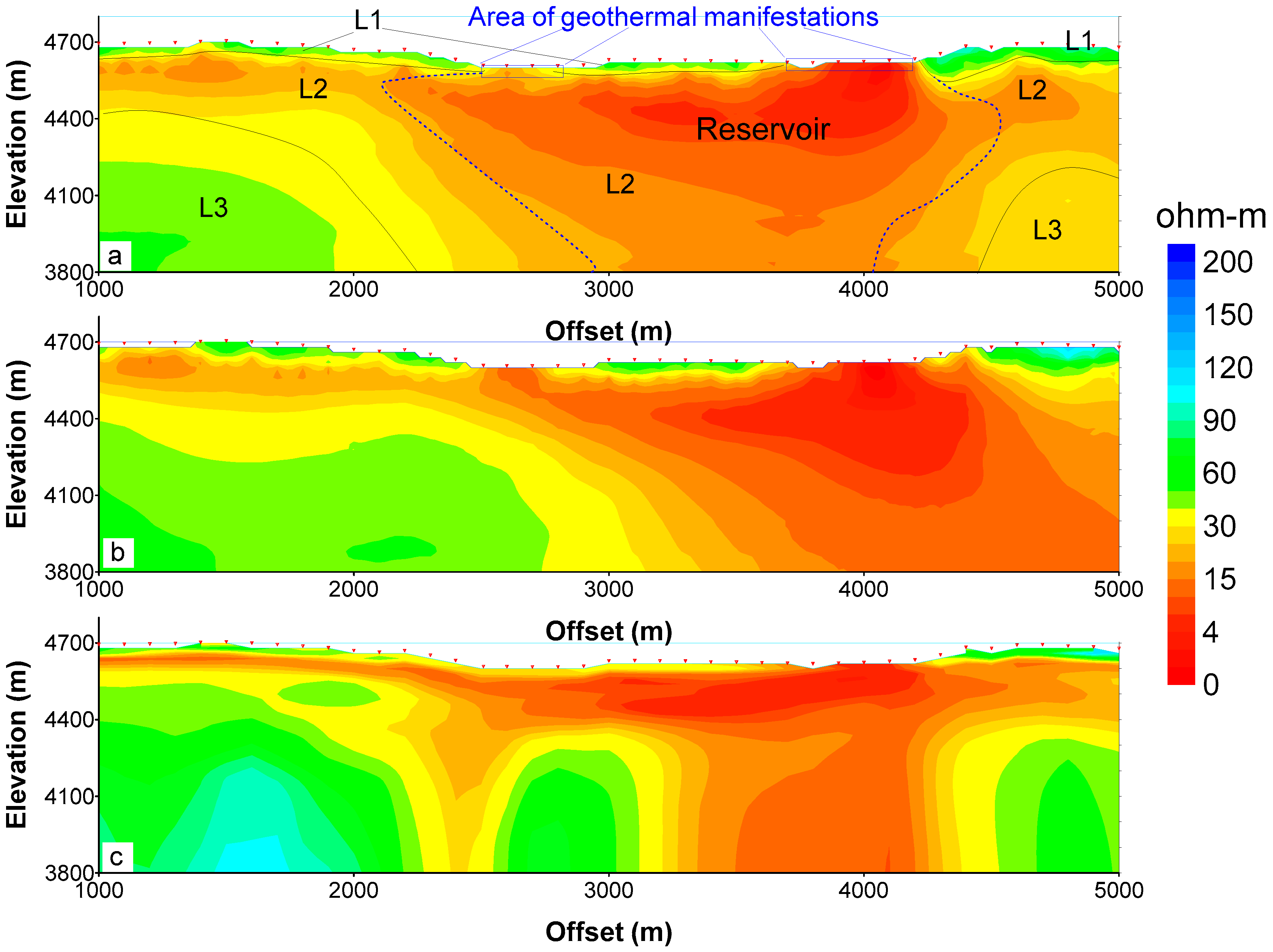
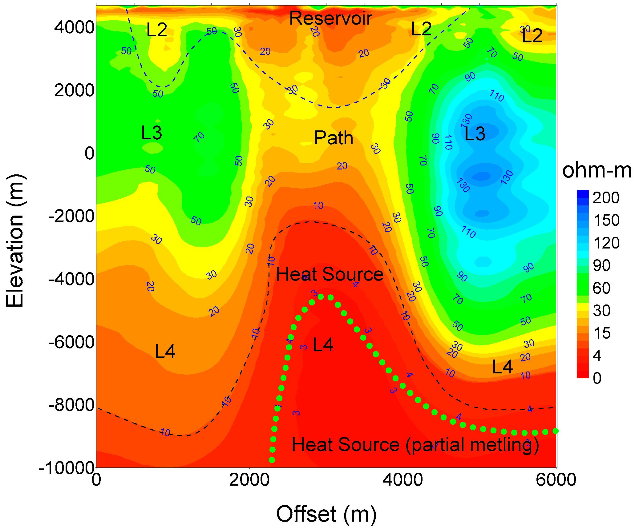
5.1. Geoelectric Structure of the Geothermal System

Southwestern Tibet is very active tectonically because of the ongoing collision between the Indian and Asian continental plates [27]. Thus, the geo-electric (resistivity) structure of the geothermal field in this region is controlled mainly by tectonic structure and distribution of thermal water. In areas where geothermal circulation and related alteration take place at depths less than 1.5 km, the investigation depth provided by the AMT method is inadequate. In these situations, the MT method provides the most suitable survey approach for mapping the geo-electric structure of deeper geothermal reservoirs [28]. Our 2D AMT and MT inversion (or conversion) results identified four distinct resistivity layers in the QP geothermal field (Figure 3 and Figure 4). These include a surface resistive layer (L1, with the exception of some surface geothermal spots), a conductive second layer (L2), a deep resistive layer (L3), and an even deeper conductive layer (L4). Of these, the thin surface resistive layer (L1) reflects the Quaternary sedimentary system in the area, and reveals lateral variations from clay to detritus deposits. The conductive second layer (L2) reflects the reservoir containing hydrothermal water and brine, as well as the formation of sandstones, shales, mudstones, and gravel-bearing sandstones. The deep resistive layer (L3) mainly reflects dry igneous rocks, while the deepest conductive layer (L4) may possibly reflect wet or partially-melting igneous rock (note that there is no direct proof of this supposition). Although the QP geothermal field can be characterized as a non-volcanic geothermal region [29], with the exception of its very resistive surface layer, this field has a similar geoelectric structure to Newberry volcano in Oregon, USA [28], and to the Theistareykir geothermal area in Iceland [30], apart from the very resistive surface layer. These sites are also characterized by the presence of a very resistive surface layer (1); a conductive layer (2); a thick resistive layer (3); and a lower-crustal conductive layer (4) [31]. Comparison of the example MT curve between Newberry volcano in Oregon and QP in Tibet is shown in Figure 7. The results indicate a similar structure, but the resistive layer of Newberry volcano develops in the frequency range of 0.01 to 0.3 Hz, while those of QP are 0.03 to 1 Hz.

5.2. The Geothermal Reservoir

On the basis of the geo-electric structure and comparisons with the geo-electric characteristics of known geothermal features, the low resistivity (conductive) layer can be interpreted as the geothermal reservoir. The distribution and resistivity features of the QP field geothermal reservoir along the survey line are shown in Figure 3a and Figure 4; results show that the reservoir along this survey line has a width of around 2200 m and a resistivity in the range 1–10 Ω∙m. The buried depth and thickness of this geothermal system are shown in Figure 3, Figure 4 and Figure 6; in general, the base of the upper thermal layer (the reservoir) is situated in the depth range 200–2200 m and is formed from sandstone, the deposition of silicides, and a clay cap formed from the alteration of rocks by hydrothermal fluids and thermal water. Results also show that the two surface geothermal features in this area derive from the same geothermal reservoir (Figure 4, Figure 5 and Figure 6). Based on inversion results and our interpretation of MT data, massive areas of remarkably high conductivity are seen within the survey area at depths in the range 0.2–2 km (Figure 4). As this high conductivity anomaly extends to the northwest beyond our last MT survey line (Figure 5a), this represents an area for future work and the potential of an additional geothermal reservoir.

Evaluating the reservoir temperature is a key issue when mapping the geothermal system. Many references in the literature are concerned with the relationship between resistivity and rock temperature [7,28,30,32,33]. To map a temperature distribution based on MT and AMT results is problematic because too many factors can influence the electrical properties of rocks [30]. Wilt and Alumbaughe [34] tested electrical resistivity as a function of temperature, porosity, and water saturation in water-flooded sandstone cores, and showed that it is highly sensitive to variations in reservoir conditions. The resistivity decreases with increasing porosity, brine saturation, and temperature, it is possible to relate these variations to geothermal reservoir temperature if a practical calibration is available on the basis of a log, modelling, or observational data. Kahwa [33] reported a temperature-resistivity model for the Theistareykir high-temperature geothermal area in Northeastern Iceland and showed that at depths less than 2000 m, a reservoir temperature of 200 °C is characterized by resistivity of less than 10 Ω∙m, while a temperature in the range 200–300 °C is characterized by a resistivity of less than the range 10–30 Ω∙m. In the QP geothermal field, resistivity of the reservoir is in the range of 2–20 Ω∙m (Figure 4, Figure 5 and Figure 6). The geological data indicate that the temperature of this geothermal reservoir is approximately 220 °C [17]. DorJi and Zhao [35] reported temperatures as high as 329 °C below a depth of 1850 m in the Yangbajing geothermal field, Tibet, an area that has a similar geothermal background to the QP field. Based on our resistivity model, the geochemical thermometer, and results from a similar geothermal field, we estimate the temperature of the QP reservoir to be in the range 200–300 °C at depths less than 3000 m.

5.3. Heat Source of the Geothermal System

The QP geothermal field is situated in the western portion of the Himalayan geothermal belt (HGB), which extends about 2000 km across Southern Tibet along the Inida-Yaluzanbo suture [36]. Magmatic activity in this area has been quite extensive since the Middle Paleocene as the Indian continental plate has moved northwards leading to closure of the Tethys Ocean by the Eurasian continental plate [35]. This subduction produced huge volumes of anatectic magma and a high background heat flow, resulting in melting of the lower crust [35,36,37]. Our MT results for the QP geothermal field revealed a deeply buried anomaly of low resistivity in the range 1–8 Ω∙m at a depth of greater than 7000 m (Figure 3 and Figure 6). The resistivity of this body is lower than that of the surrounding host rocks (40–150 Ω∙m), inferred thermal path (16–25 Ω∙m), and even the geothermal reservoir (Figure 4). Reflecting the partial melting is the most reasonable interpretation to the low-resistivity anomaly. It has a resistivity even lower than the hot brine water in the reservoir. At a depth of lower than 7 km, a cold magma or rock mass is difficult to account for the very low resistivity and very hot heat source. Additionally, a fault model is hard to explain the relative high resistivity in the path of the geothermal system. As there is no direct evidence to verify the identity of this low resistivity body, we refer to previous research in this area.

Firstly, it is generally accepted that granitic magma from the lower crust serves as the geothermal heat source for HGB, although debates continue regarding its depth and age. Geophysical data indicate the existence of a potential magmatic heat source, a 20 km thick unit of molten granite that retains water in the depth range 15–25 km at Yangbajing [38,39,40]. Duoji and Zhao [35] noted that this magma should be present in the depth range 4–5 km in the Yangbajing geothermal field, while another MT survey reflected a partially molten water-retaining granite in the depth range 9–15 km at Yangyi that has a resistivity of 3–10 Ω∙m [38]. Wang et al. [41] also reported new petrological and geochemical data from magmas that erupted 4.7–0.3 Ma in Central and Northern Tibet to demonstrate that low-velocity–high-conductivity zones can be sources of partial melting in the depth range 15–50 km. Li et al. [42] provided evidence from active hydrothermal fluids to characterize the partial melting layer in the upper crust in southern Tibet, and discussed the use of helium isotope compositions of hot spring gases and the geochemical features of spring water as approaches to model the temperature field of a geothermal reservoir. Li et al. [42] have also indicated that almost all geothermal fields with a surface temperature greater than 60 °C and geothermal features with temperatures greater than 80 °C can be used to delineate the distribution of deeply-buried magma. Thus, as the QP geothermal field is characterized by water temperatures up to 95 °C and is a typical geothermal field with hydrothermal explosions, it must have a powerful heat source, such as shallow buried high-temperature magma. Such a source would be required to heat the hydrothermal fluid and trigger flash evaporation to cause explosions.

Secondly, the presence of CO₂ in hydrothermal waters across the QP geothermal field implies a magmatic or metamorphic origin [17]. This conclusion is supported by the fact that ³He/⁴He ratios in geothermal springs along a 500 km segment of the Karakorum fault, running through the QP geothermal field, occur at 3–100 times the normal ratios found continental crust, unequivocal evidence that a component of this hydrologic system is derived from the tectonically-active mantle [43]. Indeed, Karakorum fault provides a path for upwelling of this magma. We consider that the deeply-buried low-resistivity anomaly recovered by our results at a depth greater than 7 km reflect partially melting magma, the heat source of the QP geothermal field in Southwestern Tibet. In addition, the existence of this low resistivity anomaly provides new evidence in support of the occurrence of partially melted magma in the upper crust in Southwestern Tibet.

6. Conclusions

We report the results of an exploration survey using AMT and MT methods to explore the QP geothermal field in Southwestern Tibet. Our results provide a resistivity model in the form of profile sections, contour maps at different elevations above sea level, and 3D images that enable a clearer understanding of the reservoir, the thermal path, and the heat source of the QP geothermal system. Comparison of data inversions suggests that Bostick conversion with an EMAP filter could yield reasonable frequency-to-depth conversion for the AMT and MT data. The QP geothermal system comprises four geoelectric layers extending from the surface to depths of more than 10 km, sharing similar geoelectric structural features with volcanoes in the USA and Iceland. Data demonstrate that the reservoir of the QP geothermal field extends to a depth of more than 2 km and a resistivity of 5–20 Ω∙m. A low resistivity anomaly, at a depth of more than 7 km and with a resistivity of 1–8 Ω∙m, is interpreted as the reflection of the potentially partially melted magma in the upper crust. This magma serves as the heat source for this geothermal system and is likely related to the mantle by the Karakorum Fault which passes through the middle of the QP field. Results of this AMT and MT survey provide potential geophysical evidence that help to understand the occurrence of partially melted magma in the upper crust in Southwestern Tibet.

References

1. McGlade, C.; Ekins, P. The geographical distribution of fossil fuels unused when limiting global warming to 2 °C. Nature 2015, 517, 187–190. [Google Scholar] [CrossRef] [PubMed]
2. Barbier, E. Geothermal energy technology and current status: An overview. Renew. Sustain. Energy Rev. 2002, 6, 3–65. [Google Scholar] [CrossRef]
3. Ganguly, S.; Kumar, M.M. Geothermal reservoirs—A brief review. J. Geol. Soc. India 2012, 79, 589–602. [Google Scholar] [CrossRef]
4. Fridleifsson, I.B. Geothermal energy for the benefit of the people. Renew. Sustain. Energy Rev. 2001, 5, 299–312. [Google Scholar] [CrossRef]
5. Bertani, R. Geothermal power generation in the world 2005–2010 update report. Geothermics 2012, 41, 1–29. [Google Scholar] [CrossRef]
6. Binley, A.; Cassiani, G.; Deiana, R. Hydrogeophysics: Opportunities and challenges. Boll. Geofis. Teor. Appl. 2010, 51, 267–284. [Google Scholar]
7. Spichak, V.; Manzella, A. Electromagnetic sounding of geothermal zones. J. Appl. Geophys. 2009, 68, 459–478. [Google Scholar] [CrossRef]
8. Munoz, G. Exploring for geothermal resources with electromagnetic methods. Surv. Geophys. 2014, 35, 101–122. [Google Scholar] [CrossRef]
9. Pina-Varas, P.; Ledo, J.; Queralt, P.; Marcuello, A.; Bellmunt, F.; Hidalgo, R.; Messeiller, M. 3-D Magnetotelluric exploration of Tenerife geothermal system (Canary Islands, Spain). Surv. Geophys. 2014, 35, 1045–1064. [Google Scholar] [CrossRef]
10. Wu, G.J.; Hu, X.Y.; Huo, G.P.; Zhou, X.C. Geophysical exploration for geothermal resources: An application of MT and CSAMT in Jiangxia, Wuhan, China. J. Earth Sci. 2012, 23, 757–767. [Google Scholar] [CrossRef]
11. Yin, A. Cenozoic tectonic evolution of the Himalayan orogen as onstrained by along-strike variation of structural geometry, exhumation history, and foreland sedimentation. Earth Sci. Rev. 2006, 76, 1–131. [Google Scholar] [CrossRef]
12. Kapp, P.; Murphy, M.A.; Yin, A.; Harrison, T.M.; Ding, L.; Guo, J.H. Mesozoic and Cenozoic tectonic evolution of the Shiquanhe area of western Tibet. Tectonics 2003, 22. [Google Scholar] [CrossRef]
13. Hou, Z.Q.; Zheng, Y.C.; Zeng, L.S. Eocene-Oligocene granitoids in southern Tibet: Constraints on crustal anatexis and tectonic evolution of the Himalayan orogeny. Earth Planet. Sci. Lett. 2012, 349–350, 38–52. [Google Scholar] [CrossRef]
14. Zhou, M.F.; Robinson, P.T.; Malpas, J.; Edwards, S.J.; Qi, L. REE and PGE geochemical constraints on the formation of dunites in the Luobusa ophiolite, Southern Tibet. J. Petrol. 2005, 46, 615–639. [Google Scholar] [CrossRef]
15. Hu, X.M.; Garzanti, E.; Moore, T.; Raffi, I. Direct stratigraphic dating of India-Asia collision onset at the Selandian (middle Paleocene, 59 ± 1 Ma). Geology 2015, 43, 859–862. [Google Scholar] [CrossRef]
16. DorJi. Geothermal resources and utilization in Tibet and the Himalayas; Presented at the Workshop for Decision Makers on Direct Heating Use of Geothermal Rrsources in Asia, UNU-GTP-SC-06-04, Tianjin, China, 11–18 May 2008.
17. Wang, P.; Chen, X.H.; Shen, L.C.; Wu, K.Y.; Huang, M.Z.; Xiao, Q. Geochemical features of the geothermal fluids from the Mapamyum non-volcanic geothermal system (Western Tibet, China). J. Volcanol. Geotherm. Res. 2016, 320, 29–39. [Google Scholar] [CrossRef]
18. Vozoff, K. The magnetotelluric method. In Electromagnetic Methods in Applied Geophysics; Investigations in Geophysics, 3, v. 2 Applications Part B; Nabighian, M.N., Ed.; Society of Exploration Geophysicists: Tulsa Oklahoma, OK, USA, 1991; pp. 641–711. [Google Scholar]
19. Tikhonov, A.N. On determining electrical characteristics of the deep layers of the Earth’s crust. Doklady Akademii Nauk SSSR 1950, 73, 295–297. [Google Scholar]
20. Cagniard, L. Basic theory of the magnetotelluric method of geophysical prospecting. Geophysics 1953, 18, 605–635. [Google Scholar] [CrossRef]
21. Peacock, J.R.; Thiel, S.; Heinson, G.S.; Reid, P. Time-lapse magnetotelluric monitoring of an enhanced geothermal system. Geophysics 2013, 78, B121–B130. [Google Scholar] [CrossRef]
22. U.S. Geological Survey. The Audio-Magnetotelluric Method (AMT). Available online: http://pubs.usgs.gov/of/2003/of03-056/html/AMTMdesc.htm (accessed on 20 July 2016).
23. He, L.F.; Feng, M.H.; He, Z.X.; Wang, X.B. Application of EM methods for the investigation of Qiyueshan Tunnel, China. J. Environ. Eng. Geophys. 2006, 11, 151–156. [Google Scholar] [CrossRef]
24. Torres-Verdin, C.; Bostick, F.X. Principles of spatial surface electric field filtering in magnetotellurics: Electromagnetic array profiling (EMAP). Geophysics 1992, 57, 603–622. [Google Scholar] [CrossRef]
25. Bostick, F.X. A Simple Almost Exact Method of MT Analysis: Presented at the Workshop on Electrical Methods in Geothermal Exploration; Contract 14-08-001-6-359; U.S. Geological Survey: Snowbird, UT, USA, 1977.
26. Rodi, W.; Mackie, R.L. Nonlinear conjugate gradients algorithm for 2-D magnetotelluric inversion. Geophysics 2001, 66, 174–187. [Google Scholar] [CrossRef]
27. Bai, D.; Unsworth, M.J.; Meju, M.A.; Ma, X.; Teng, J.; Kong, X.; Zhao, C. Crustal deformation of the eastern Tibetan plateau revealed by magnetotelluric imaging. Nat. Geosci. 2010, 3, 358–362. [Google Scholar] [CrossRef]
28. Oskooi, B.; Laust, B.P.; Smirnov, M. Electromagnetic induction in the Earth: The deep geothermal structure of the Mid-Atlantic Ridge deduced from MT data in SW Iceland. Phys. Earth Planet. Inter. 2005, 150, 183–195. [Google Scholar] [CrossRef]
29. Xiao, Q.; Wang, P.; Shen, L.C.; Xue, M. Soil CO2 degassing process and flux from the Mapamyum non-volcanic geothermal region. Geol. China 2015, 42, 2019–2028. (In Chinese) [Google Scholar]
30. Yu, G.; Gunnarsson, Á.; He, Z.X.; Tulinius, H. Characterizing a geothermal reservoir using a broadband 2-D MT survey in Theistareykir, Iceland. In Proceedings of the World Geothermal Congress, Bali, Indonesia, 25–29 April 2010.
31. Fitterman, D.V.; Stanley, W.D.; Bisdorf, R.J. Electrical structure of Newberry Volcano, Oregon. J. Geophys. Res. 1988, 93, 10119–10134. [Google Scholar] [CrossRef]
32. Bibby, H.M.; Risk, G.F.; Caldwell, T.G.; Heise, W. Investigations of deep resistivity structures at the Wairakei geothermal field. Geothermics 2009, 38, 98–107. [Google Scholar] [CrossRef]
33. Kahwa, E. Geophysical exploration of high temperature geothermal areas using resistivity methods. Case study: Theistareykir Area, NE Iceland. In Proceedings of the World Geothermal Congress, Melbourne, Australia, 19–25 April 2015.
34. Wilt, M.; Alumbaugh, D. Electromagnetic methods for development and production: State of the art. Lead. Edge 1998, 17, 487. [Google Scholar] [CrossRef]
35. Ji, D.; Zhao, P. Characteristics and genesis of the Yangbajing geothermal field, Tibet. In Proceedings of the World Geothermal Congress, Kyushu-Tohoku, Japan, 28 May–10 June 2000.
36. Liao, Z.J. Setting of the geothermal activities of Xizang (Tibet) and a discussion of the associated heat source problem. Acta Sci. Nat. Univ. Pekin. 1982, 18, 70–78. (In Chinese) [Google Scholar]
37. Tong, W.; Zhang, Z.F.; Liao, Z.J.; Zhu, M.X.; Zhang, M.T. Hydrothermal activities occurring on the Xizang (Tibetan) Plateau and preliminary discussion about the thermal regime within its upper crust. Chin. J. Geophys. Chin. Ed. 1982, 25, 34–40. [Google Scholar]
38. Guo, Q.H. Hydrogeochemistry of high-temperature geothermal systems in China: A review. Appl. Geochem. 2012, 27, 1887–1898. [Google Scholar] [CrossRef]
39. Makovsky, Y.; Klemperer, S.L.; Ratschbacher, L.; Brown, L.D.; Li, M.; Zhao, W.; Meng, F. INDEPTH wide-angle reflection observation of P-wave-to-S-wave conversion from crustal bright spots in Tibet. Science 1996, 274, 1690–1691. [Google Scholar] [CrossRef] [PubMed]
40. Zhao, W.J.; Zhao, X.; Shi, D.N.; Liu, K.; Jiang, W.; Wu, Z.H.; Xiaong, J.Y.; Zheng, Y.K. Progress in the study of deep profiles (INDEPTH) in the Himalayas and Qinghai-Tibet Plateau. Geol. Bull. China 2002, 21, 691–700. (In Chinese) [Google Scholar]
41. Wang, Q.; Hawkesworth, C.J.; Wyman, D.; Chung, S.L.; Wu, F.Y.; Li, X.H.; Dan, W. Pliocene-Quaternary crustal melting in central and northern Tibet and insights into crustal flow. Nat. Commun. 2016, 7. [Google Scholar] [CrossRef] [PubMed]
42. Li, Z.Q.; Hou, Z.Q.; Nie, F.J.; Meng, X.J. Characteristic and Distribution of the Partial Mel ting Layers in the Upper Crust: Evidence from Active Hydrothermal Fluid in the South Tibet. Acta Geol. Sin. 2005, 79, 68–77. [Google Scholar]
43. Klemperer, S.L.; Kennedy, B.M.; Sastry, S.R.; Makovsky, Y.; Harinarayana, T.; Leech, M.L. Mantle fluids in the Karakorum fault: Helium isotope evidence. Earth Planet. Sci. Lett. 2013, 366, 59–70. [Google Scholar] [CrossRef]
Figure 1. Simplified geologic map of the Himalayas to show the locations of the study area, the QP geothermal field, the Karakorum fault, and the Indus-Yarlung Zangbo suture zone (modified from Hu et al. [15]).
Energies 09 00855 g001
Figure 2. Location of the QP geothermal field and field layout of AMT and MT survey. (a) Location of the QP geothermal field; (b) its geological setting; (c) cross section; (d) locations of geothermal features; (e) the local geological map showing field layout; and (f) the location of the hot springs in Tibet (modified from Wang et al. [17], with permission from the authors). Line1 and Line2 show the location of the section of Figure 3 and Figure 4. Numerals: (1) Late Holocene alluvial-proluvial fan; (2) Pleistocene deposits; (3) Lower Member of the Neocene Woma Group; (4) Upper Cretaceous Sangdanlin Formation; (5) Upper Carboniferous Lasha Formation; (6) Lower Carboniferous Kangtuo Formation; (7) Neocene monzogranite granite; (8) Upper Triassic mafic rocks; (9) Upper Triassic complex; (10) Quaternary sediment; (11) conglomerate; (12) sandstone; (13) mudstone; (14) shale; (15) siliceous rock; (16) complex rock; (17) mafic rock; (18) phyllite; (19) meta-sandstone; (20) metamorphic conglomerate; (21) mylonite; (22) monzogranite; (23) boundary of an unconformity; (24) reverse fault; (25) buried fault; and (26) stream or lake.
Energies 09 00855 g002
Figure 3. Comparison between Bostick conversion of (a) the XY direction, (b) the YX direction, and (c) nonlinear conjugate gradient inversion (NLCGI) results for an AMT section ((Line1 as shown in Figure 2 and Figure 5). The black solid line outlines the geo-electric layers (L1 to L3). The blue dashed line shows the geothermal reservoir interpreted from the AMT results.
Energies 09 00855 g003
Figure 4. Conversion results from a MT section (Line2 as shown in Figure 2 and Figure 5) illustrate the typical geo-electric structure of the QP geothermal field. L2 to L4 show the geo-electric layer, L2 is a low-resistivity layer mainly reflecting the reservoir (marked with the blue dashed line) which contains the brine thermal fluids (water); L3 is a resistive layer that reflects the host rock and path (has lower resistivity than the host rocks); L4 is a low resistivity layer, which the major portion reflects the heat source (marked with the black dashed line). The lower portion of L4 (marked with the green dashed line) is interpreted as partial melting.
Energies 09 00855 g004
Figure 5. Resistivity contour maps at elevations of (a) 3500 m and (b) 2000 m ASL. The reservoir and the thermal path of the geothermal system are outlined with the blue dashed line. Line1 and Line2 show the location of the section of Figure 3 and Figure 4. The red rectangle shows the portion where three-dimensional imaging is conducted and shows in Figure 6.
Energies 09 00855 g005
Figure 6. 3D resistivity imaging shows the resistivity volume with a value lower than (a) 15 and (b) 22 Ω∙m for the eastern portion of the QP geothermal field. A low-reisitivity volume with a value lower than 15 Ω∙m (a) reflects the heat source and upper portion of geothermal reservoir, another data volume of lower than 22 Ω∙m reflects the whole geothermal system, including the heat source, path, and the reservoir. The path has a higher resistivity of 15–22 Ω∙m than the heat source and the reservoir.
Energies 09 00855 g006
Figure 7. Comparison of example MT sounding curves from QP, Tibet, and the Newberry volcano, Oregon, USA. The foot figure shows the curve from Newberry volcano, the black triangles are resistivity and phase of MT XY direction, and the square are resistivity and phase of MT YX direction [28]. The blue dot and red brick show the resistivity and phase of the MT XY direction of one station in QP.
Energies 09 00855 g007