Article

A Novel Data Hierarchical Fusion Method for Gas Turbine Engine Performance Fault Diagnosis

1
Jiangsu Province Key Laboratory of Aerospace Power Systems, College of Energy & Power Engineering, Nanjing University of Aeronautics and Astronautics, Nanjing 210016, Jiangsu, China
2
Department of Mechanical and Industrial Engineering, University of Toronto, Toronto, ON M5S 3G8, Canada
3
Aviation Motor Control System Institute, Aviation Industry Corporation of China, Wuxi 214063, Jiangsu, China
*
Author to whom correspondence should be addressed.
Energies 2016, 9(10), 828; https://doi.org/10.3390/en9100828
Submission received: 27 July 2016 / Revised: 27 September 2016 / Accepted: 11 October 2016 / Published: 15 October 2016

Abstract

:
Gas path fault diagnosis involves the effective utilization of condition-based sensor signals along engine gas path to accurately identify engine performance failure. The rapid development of information processing technology has led to the use of multiple-source information fusion for fault diagnostics. Numerous efforts have been paid to develop data-based fusion methods, such as neural networks fusion, while little research has focused on fusion architecture or the fusion of different method kinds. In this paper, a data hierarchical fusion using improved weighted Dempster–Shaffer evidence theory (WDS) is proposed, and the integration of data-based and model-based methods is presented for engine gas-path fault diagnosis. For the purpose of simplifying learning machine typology, a recursive reduced kernel based extreme learning machine (RR-KELM) is developed to produce the fault probability, which is considered as the data-based evidence. Meanwhile, the model-based evidence is achieved using particle filter-fuzzy logic algorithm (PF-FL) by engine health estimation and component fault location in feature level. The outputs of two evidences are integrated using WDS evidence theory in decision level to reach a final recognition decision of gas-path fault pattern. The characteristics and advantages of two evidences are analyzed and used as guidelines for data hierarchical fusion framework. Our goal is that the proposed methodology provides much better performance of gas-path fault diagnosis compared to solely relying on data-based or model-based method. The hierarchical fusion framework is evaluated in terms to fault diagnosis accuracy and robustness through a case study involving fault mode dataset of a turbofan engine that is generated by the general gas turbine simulation. These applications confirm the effectiveness and usefulness of the proposed approach.

1. Introduction

Gas turbine engine provides power for airplane, and its reliable operation plays an important role in flight safety. Due to the complexity of structure and terrible work condition, gas turbine engine has more opportunity to break down [1]. Engine failures is generally divided into gas-path performance fault, vibration structure fault and auxiliary system fault, among which the performance fault causes more maintenance costs and off-wing time [2]. Engine performance fault diagnosis is one of the key technologies to support advanced condition-based maintenance strategies and has received a wide interest, with great potential to reduce engine maintenance costs and improve availability [3,4]. It is important to develop methodologies to improve the confidence of performance fault diagnosis for gas turbine engine using various kinds of available sensors.
Numerous approaches have been developed for engine health monitoring and gas-path fault diagnosis, such as the model-based methods (nonlinear least square, and Kalman filter) [5,6,7,8,9,10,11], data-based methods (artificial neural networks, fuzzy logic, rough sets and decision tree, and expert systems) [12,13,14,15,16]. The model-based method has been employed for engine gas-path fault diagnosis since 1970s, and the unmeasured component performance shifts are estimated from the residuals between the engine model outputs and sensed signals. Urban proposed a linearized model-based method using nonlinear least square for gas-path analysis (GPA) [17], and it is the first time to produce the estimates of fault feature parameter from observable measurements. In order to improve estimation accuracy, the state estimator based methods such as various Kalman filter (KF) and Particle filter (PF), are then introduced to engine health estimation. In the past twenty years, varieties of KF have been widely used for engine performance estimation and gas path fault diagnosis [7,8], and it is illustrated in Figure 1. In order to address engine nonlinearity in the health estimation, nonlinear model-based methods are developed using extended Kalman filter, unscented Kalman filter and PF [9,18,19]. These model-based methods performs well in some conditions, whereas their performance closely relies on the engine model precision [20,21]. It is difficult to obtain an accurate engine model to describe the dynamic and steady behavior at various operating conditions in whole flight envelope, and the modeling mismatch will bring false diagnosis.
The data-driven method is another significant way to complete engine gas-path fault diagnosis. Neural network (NN) is a well-known learning machine, and it is also an important data-based method applied to detect and isolate engine component and sensor faults [13]. Variants of the NNs are fulfilled with the goal of the smallest empirical risk, and the dimension disaster or over-fitting might occur due to a large number of samples required [22,23]. Support vector machine (SVM) is proposed on the basis of the minimum structural risk in the last twenty years, and this statistical learning approach has strictly mathematical deduction [24,25]. The SVM is employed to monitor gas turbine performance degradation, and it is proved to be superior to the basic NN with classification capability and generalization performance regards [26]. Kernel extreme learning machine (KELM) is recently developed from the NNs and SVM with kernel transformation, and it has less coefficients need to be calculated in the training process simple topology [27]. The KELM is used to feature extraction, pattern recognition and fault diagnosis.
However, the original KELM is lack of sparseness, which makes its topological structure complexity grow with sample size. It affects the real-time capability of the KELM. Thus choosing suitable samples to realize sparseness of KELM plays a key role in training KELM in the cases of large-scale datasets. At the aim of simplified KELM topology, some studies on pruning techniques have been done [28,29], but these variations focus on structure sparseness not data sparseness. Since there is a one-to-one correspondence between a hidden node and a sample In KELM, it is possible to achieve sparsity in terms of training data. A sparse ELM (S-ELM) algorithm is proposed to greatly reduce the storage space and forecasting time, and it replacing the equality constraints by inequality constraints [30]. Then a fast sparse approximation scheme of extreme learning machine (FSA-ELM) is proposed [31], and it has the features of low complexity and sparse solution. FSA-ELM defines one basis function for each sample in the training set and iteratively builds the decision function by adding one basis function from the kernel-based dictionary. However, the constraints brought by samples that are not selected to the decision function are not considered, and the problem of weight between the topology sophistication and prediction accuracy rises up. For the purposes of simplifying KELM topology with less reduction of accuracy, the RR-KELM is proposed on the basis of the FSA-ELM using a reduced technique in this paper.
When the in-flight performance fault diagnosis for gas turbine engine is concerned, the confidence requirements of fault pattern recognition increases. The sensor fusion technologies using learning machine are developed, such as the integration of multiple types NNs, or combination of NN and fuzzy logic [32,33]. The essence of these fusion approaches are the data-based ones, and aero-thermodynamic characteristics of gas turbine engine is not taken into account [34]. These data-based sensor fusion methods would be still failed to new fault modes due to the lack of very training samples. In this paper, the combination of model-based and data-driven using weighted Dempster–Shaffer evidence theory (WDS) with different feature information in data hierarchical fusion framework is developed. Our main objective in this work is to develop a data hierarchical fusion framework to improve the performance of in-flight gas-path fault diagnosis. One model-based evidence is brought by the PF-FL algorithm in feature level, and the other data-based evidence one produced by the RR-KELM. A final decision of performance fault pattern for airplane engine is achieved from two evidences using information fusion scheme in decision level. To confirm the effectiveness of the proposed methodology, turbofan engine data from a general gas turbine simulation are applied to carry out experiments. From these reports, it is easily got that the data hierarchical fusion method has satisfactory confidence of performance fault diagnosis.
The paper is organized as follows. The problem formulation is given, and the RR-KELM is proposed to produce one data-based evidence of gas-path fault diagnosis in feature level in Section 2. The model-based method using PF-FL is then discussed to produce another evidence, and the WDS and data hierarchical fusion mechanism for gas-path fault diagnosis are developed in Section 3. Section 4 shows the simulation and analysis, and it indicates the performance of the data hierarchical fusion framework using the WDS is improved in respects of fault diagnosis accuracy and robustness. Section 5 draws a conclusion and discussed future research directions.

2. Data-Based Fault Diagnosis Using the RR-KELM

Gas turbine engine is a complex mechanical system, and in this paper a two-spool mixing-exhaust turbofan engine is studied. The engine mainly includes the following components: Inlet, Fan, Compressor, Combustor, High-Pressure Turbine (HPT), Low-Pressure Turbine (LPT), Bypass, Mixing Chamber and Nozzle [35,36]. Figure 2 gives the schematic representation of the examined gas turbine engine. The airflow is driven into the fan after through an inlet. It is then separated into two streams before the compressor: one stream passes through the annular bypass duct and the other through the engine core. Fuel is sprayed into the combustor, mixed with the air from the compressor and burned to produce hot gas to drive the turbines. There are two spools, through which the high pressure turbine (HPT) drives compressor, and the low pressure turbine (LPT) drives fan. The gas leaves the LPT and mixed the air from the bypass in the mixing chamber. The mixed gas is guided into the nozzle at last, and it has a variable throttle area.
Engine gas-path fault results from fouling, leakage, erosion, corrosion, seal damage, foreign and domestic objective damage, and hot end components damage, and it becomes serious with the increase of usage cycle number. The deviation of health parameter is called fault feature parameter, which is used to quantitatively represent engine gas-path fault modes. The fault feature parameters include the deviations of fan efficiency SE1, compressor efficiency SE2, HPT efficiency SE3 and LPT efficiency SE4, which cannot be directly measured. As we know, gas-path fault causes the sensed parameters change, then the measurement deviation could be used to calculate fault feature parameter. The engine measurements include low-pressure spool speed NL, high-pressure spool speed NH, fan outlet temperature T22, fan outlet pressure P22, compressor outlet temperature T3, compressor outlet pressure P3, LPT inlet temperature T43, and LPT outlet temperature T6. The elements of control vector are fuel flow Wf and nozzle area A8, which determine the engine operating conditions. In this section, the RR-KELM algorithm is proposed and employed to achieve the classification of gas-path fault modes, and the fault mode identification result is served as data-based evidence.

2.1. KELM

The KELM is developed from the ELM with the kernel transformation method, and it brings better generalization than the ELM in the most applications due to the kernel transformation to the feature space [27,37]. Assume the training set of KELM = { ( x i , y i ) | x i R n , y i R , i = 1 , 2 , , N } . The learning problem of KELM is to search an optimal function F: xiyi, and it is presented by F ( x i ) y i . Once an activation function gi() and hidden neuron number L is given, the function F() is expressed
y = F ( x ) = i = 1 L β i g i ( x ) =   G ( x ) T   β  
where β = [β1, β2, …, βL]T is output weights from the hidden neurons to output nodes, and G(x) = [g1(x), g2(x), …, gL(x)]T is output vector of the hidden neurons corresponding to input x. For the general ELM optimization theory, it is to search the optimal output weights to produce the minimum of empirical risk and structural risk, and the risk function is R = β + C G T β y . Thus the learning problem of ELM is converted
min β 1 2 β 2 2 + C 2 i = 1 N ε i 2 s . t . G T ( x i ) β = y i ε i , i = 1 , 2 , , N
where the penalty factor C is a trade-off between output weights norm and fitting error, and the slack variable ε i implies the differences between predicted and actual value. Given the output vector is y = [y1, y2, …, yN]T, the optimal output weight of ELM in Equation (2) is written
β = G ( 1 C I N + G T G ) 1 y
Comparing to the basic ELM, a regularization term 1 C I N is added to the KELM. Besides, the kernel transformation k ( x i , x j ) , namely a mapping from input space to feature space, replaces an explicit activation function in the hidden layer of the ELM
Κ i , j = G T ( x i ) G ( x j ) = k ( x i , x j ) k ( x i , x j ) = exp ( γ x i x j 2 )
where the kernel parameter γ is the kernel distribution width. The KELM function in Equation (1) can be calculated as follows
F ( x ) = G T ( x ) β = G T G ( 1 C I N + G T G ) 1 y = k ( x ) α α = ( 1 C I N + Κ ) 1 y
where α is the output weight of the KELM. It is noted that the number of hidden nodes in KELM equals to the training sample count. When it comes to the large-scale datasets, especially in the cases of performance fault diagnosis at various operating conditions in whole flight envelope, the topological structure of KELM might be redundant. Then the sparsity of KELM is emerged, and it affects not only real-time calculation but also the generalization performance for gas-path fault diagnosis.
A fast sparse approximation (FSA) scheme is developed to the problem that the model scale grows hazard as sample size increase [31]. Provided a kernel function k ( x , x i ) is one basis function for each sample xi in the training set, a set of basis functions D = { k ( x , x i ) | i = 1 , , N } is called a kernel-based dictionary. FSA-ELM is a greedy algorithm which iteratively builds the decision function by adding one basis function from the kernel-based dictionary at one time. The key of FSA-ELM is to select the basis function. The FSA-ELM starts from an empty index set P = and a full index set Q = { 1 , 2 , , N } , and selects a new basis function k ( x , x s ) from the set { k ( x , x i ) | i Q } . It provides insights into simplifying the topological structure of KELM.

2.2. RR-KELM

Given a random small-scale subset X s = { x i } i = 1 s is selected from the original N data points X = { x i } i = 1 N with s N using this reduced technique, and the learning problem Equation (2) is regulated for the reduced dataset as follows
min α { L s = 1 2 α T K S S α + C 2 i = 1 N [ y i j S α j k ( x j , x i ) ] 2 }
where K S S ( i , j ) = k ( x i , x j ) , i , j S . Since the number of training sample is s less than that of basic KELM, the hidden neuron count is s and the topology of learning machine is simplified compared to the original KELM topology. The optimization target keeps the N constraints of the whole dataset, and it helps to enhance the generalization performance.
Let L s α = 0 in Equation (6), we have
( K S S / C + K S N K S N T ) α = K S N y
where K S N ( i , j ) = k ( x i , x j ) , i S , j = 1 , 2 , , N . Note that this reduced technique might produce lower testing accuracy than basic K-ELM due to randomly selecting the subset of training data.
On the other hand, FSA-ELM presented a strategy of selecting the optimal kernel functions. Nevertheless, the defect of FSA-ELM is that the contribution of the rest non-selected data is not considered to the output weights. Therefore, the RR-KELM is proposed from the FSA-ELM using the reduced technique. The reduced training samples technique that includes the whole N constraints information is discussed, and the iterative calculation strategy is combined in RR-KELM.

2.2.1. Strategy of Selecting the Reduced Subset

When the kernel function of a new basis k(x, xi) is determined at the (n + 1)-th iteration, the optimization target function Equation (6) can be reformulated as
min α s { L s = 1 2 α T ( K S S / C + U S S ) α α T K S N y } min α s { L s = 1 2 [ α n T α i ] ( [ K S S / C k ¯ i k ¯ i T k ( x i , x i ) / C ] + [ U s s u i u T i U i i ] ) [ α n α i ] [ α n T α i ] [ K S N K i N ] y }
where U S S = K S N K S N T , and the output weights vector α n = [ α 1 , α 2 , , α n ] T at the n-th iteration. The expressions follow k ¯ i = [ k ( x s 1 , x i ) , k ( x s 2 , x i ) , , k ( x s n , x i ) ] T / C , s 1 , s 2 , , s n S , K i N = [ k ( x 1 , x i ) ​  , k ( x 2 , x i ) , , k ( x N , x i ) ] T , u i = K S N K i N T , U i i = K i N K i N T . The candidates of basis function have little effects on the selected training samples, and the output weights in α n are fixed and Equation (8) is further simplified
min α i { L s = ( k ( x i , x i ) / C + U i i ) 2 α i 2 + r i α i }
r i = { y ^ i , n = 0 ( k ¯ i T + u T i ) α n y ^ i , n > 0
where y ^ i = K i N y . Thus, we select the index s from Q into S based on the following criterion
s = arg min i Q ( ( r i ) 2 2 ( k ( x i , x i ) / C + k ¯ i T k ¯ i ) )
The stopping condition of iteration is
max ( | r Q | ) < δ  or  n > M
where δ is a small positive constant, n is total number of selected basis functions, and M is the maximum subset.

2.2.2. Iterative Computation of the Kernel Matrix Inversion

Let R = ( K S S / C + U S S ) 1 , the solution of Equation (11) is
α s n = R K S N y
A new sample xi is picked up at the (n + 1)-th iteration, and the expression is as follows
R n + 1 = [ [ K s s / C k ¯ i T k ¯ i k ( x i , x i ) / C ] + [ U s s u T i u i U i i ] ] 1
Theorem 1.
Given an arbitrary invertible matrix A and matrices D, V, U, the following expression holds
[ A U V D ] 1 = [ A 1 + A 1 U ( D V A 1 U ) 1 V A 1 - A 1 U ( D V A 1 U ) 1 - ( D V A 1 U ) 1 V A 1 ( D V A 1 U ) 1 ]
Let β = R n ( k ¯ i + u i ) , λ = ( k ( x i , x i ) / C + U i i ( k ¯ i T + u i T ) β ) , and then Equation (13) is rewritten using Theorem 1
R n + 1 = [ R n 0 0 0 ] + λ [ β 1 ] [ β T 1 ]
Combining the iterative computation of the kernel matrix inversion with the strategy of selecting reduced subset, the proposed RR-KELM is described in the following.
Algorithm RR-KELM
(1)Initialization: inputs includes kernel function k(xi, xj), regularization parameter C, training set { ( x i , y i ) , i = 1 , 2 , , N } ; Output contains the output weights α computed after the last iteration.
(2)Let S = , Q = { 1 , 2 , , N } , n = 0, and define a small positive constant δ and a positive integer M.
(3)If Q = or max ( | r Q n | ) < δ or n > M stop the iteration.
(4) s = arg min i Q ( ( r i ) 2 2 ( k i i / C + k ¯ i T k ¯ i ) ) .
(5)Compute R n + 1 and α s n + 1 separately from Equations (15) and (12).
(6) Q = Q { s } , S = S + { s } .
(7) r Q ( i ) = ( k ¯ i T + u T i ) α s y ^ i , i Q .
(8)n = n + 1, go to Step 3.
As far as engine gas-path fault diagnosis, the RR-KELM input for is a 9-element vector including the engine parameters Wf, NL, NH, T22, P22, T3, P3, T43 and T6. The RR-KELM’s output is a 10-element vector of fault probability, and each element related to one engine gas-path fault pattern given in Table 1. The i-th fault mode is identified as the i-th element of fault probability vector is the maximum and more than 0.5, and the fault probability vector is used as the decision of data-based evidence.

3. Data Hierarchical Fusion for Engine Gas-Path Fault Diagnosis

Generally speaking, there are three kinds of data fusion structure, namely data-level fusion, feature-level fusion and decision-level fusion. Data-level fusion is the lowest layer information, which directly integrates multiple sensor data. A data-level fusion scheme is applied to degradation modeling and prognostic analysis for turbofan engine [32]. The original measurements are treated by extracting fault feature information, and then the information is integrated called feature-level fusion for fault diagnosis [33]. A fuzzy-based method in feature-level fusion is presented for gas turbine fault detection and identification [38]. The intermediate decision of each module combined for final decision in the topmost layer is denoted by decision-level fusion. The Dempster–Shaffer evidence theory (DS) is one of the most common fusion methods since it is simple and easy for implement. The DS has been applied for engine anomaly detection and vibration fault diagnosis [39]. The WDS in the data hierarchical fusion mechanism and the integration of two different kinds of evidences are discussed for engine gas-path fault diagnosis in this section. The fault mode index by the method-based evidence and fault mode probability by the data-based evidence are combined in the decision layer in the fusion framework.

3.1. Model-Based Fault Diagnosis Using PF-FL Method in Feature Layer

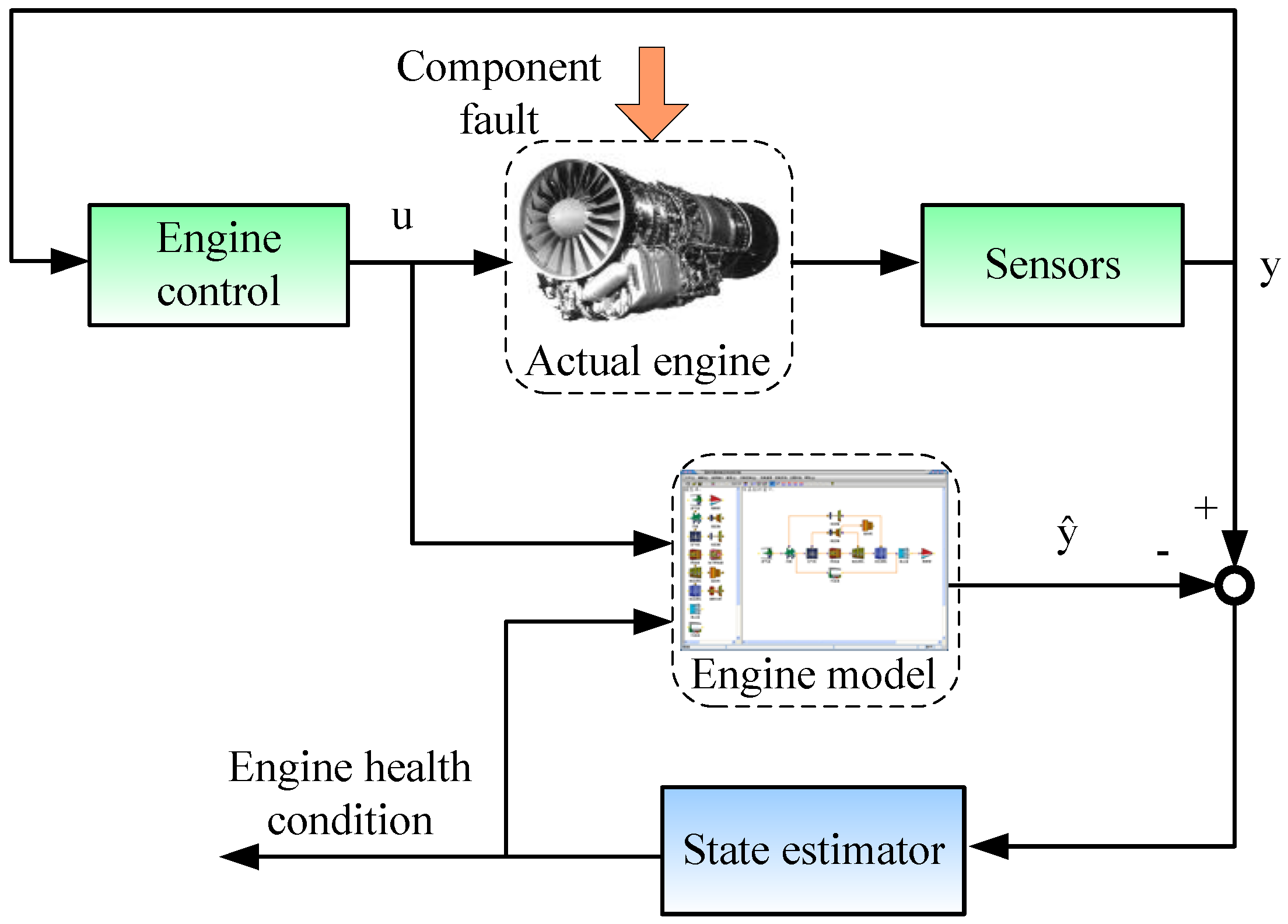
The nonlinear model-based method using PF-FL for engine gas-path fault diagnosis completes by two steps: fault feature parameter estimation and fault identification. The PF algorithm is served as a state estimator to calculate the component performance deviations from their normal values. The deviations of fault feature parameters are then fed to the fuzzy logic system for fault mode recognition. The fault mode index is computed by the PF-FL and used as the model-based evidence.
Considering air flow mass, power and momentum conservation laws, a general gas turbine engine simulation is designed [35]. The characteristic maps of engine rotating components describe aero-thermodynamic relationships of component inputs and outputs in the engine simulation [36]. The data of engine design operation and component maps are loaded to the general simulation for obtaining a turbofan engine component level model (CLM) [40]. The nonlinear mathematical model of the engine is given by
x k + 1 = f ( x k , u k ) + w k y k = g ( x k , u k ) + v k
where k is the time index, y is the 8-element measured output, x is the 6-element augmented state variable, and u is the 2-element control input. The noise terms w and v represent process uncertainty and measurement uncertainty in the model. Since the PF is based on sequential Monte Carlo sampling theory and aimed to state estimation of nonlinear and non-Gauss system [41], it is especially suitable to gas turbine engine. Hence, the PF algorithm is employed to the estimation of engine fault feature parameters.
Let x 0 : k = { x 0 , , x k } denote the series of the augmented state vector [
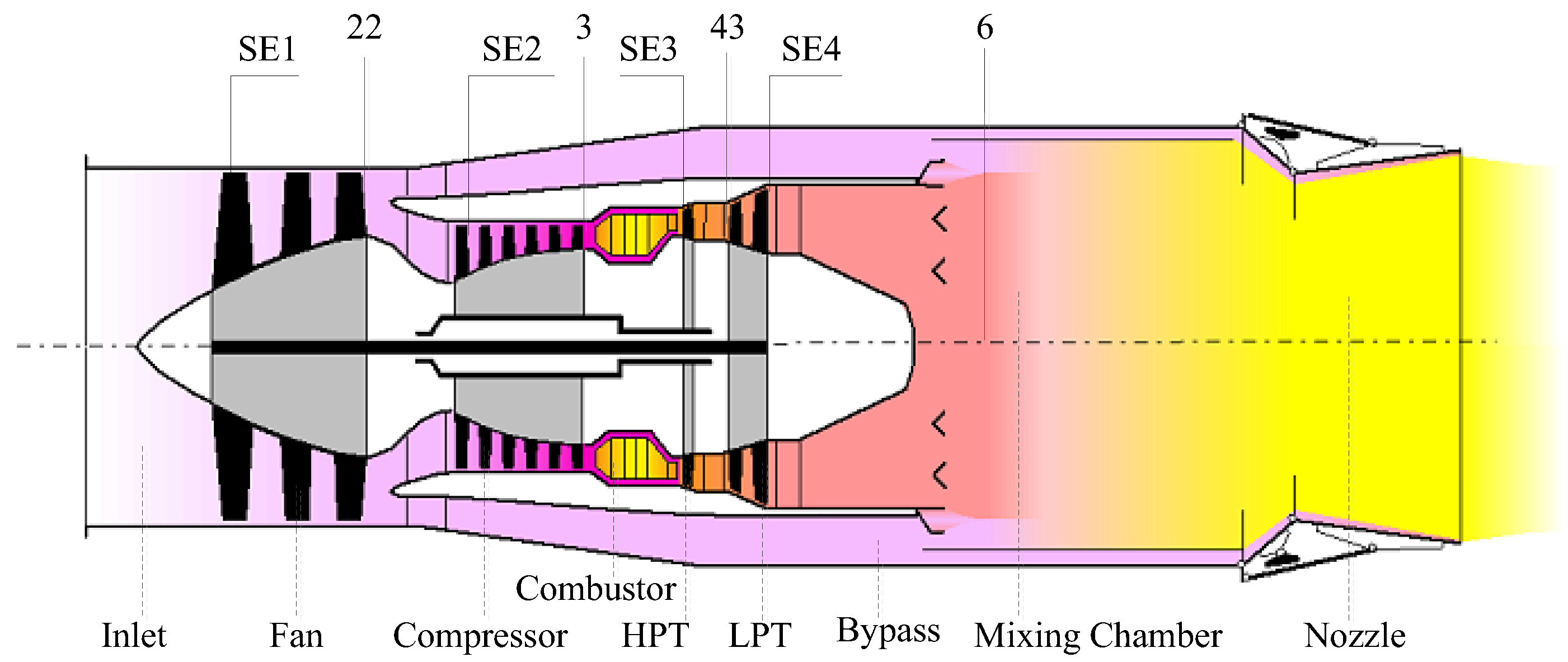
NL, NH, SE1, SE2, SE3, SE4]T, and y 1 : k = { y 1 , , y k } denote the series of measurement vector [NL, NH, T22, P22, T3, P3, T43, T6]T. Give the probability density function (PDF) of the prior condition is p(x0), and the posterior PDF p(x0:k|y1:k) is characterized by a set of weighted random samples { x 0 : k i , w k i } i = 1 N , wherein N is particle number. The particle set { x 0 : k i ; i = 0 , , N } is related to the weight { w k i ; i = 0 , , N } , and the PDF at time k is approximated by
p ( x 0 : k | y 1 : k ) 1 N w k i δ ( x 0 : k x 0 : k i ) 1 N w k i = 1
The case for Monte Carlo sampling is to generate particles from the posterior PDF p(x0:k|y1:k), but it is unavailable directly. Then the importance sampling distribution function q(x0:k|y1:k) is expressed before sampling
q ( x k | x 0 : k 1 , z 1 : k ) = q ( x k | x k 1 , z k ) q ( x k i | x k 1 i , z k ) = p ( x k i | x k 1 i )
The i-th particle weight w k i can be approximated by
w k i p ( x 0 : k | y 1 : k ) q ( x 0 : k | y 1 : k ) p ( y k | x k i ) p ( x k i | x k 1 i ) p ( x 0 : k 1 i | y 1 : k 1 ) q ( x k i | x 0 : k 1 i , y 1 : k ) q ( x 0 : k 1 i | y 1 : k 1 ) = w k 1 i p ( y k | x k i ) p ( x k i | x k 1 i ) q ( x k i | x 0 : k 1 i , y 1 : k )
The importance weights is normalized
w k i = w k i / i = 1 N w k i
There is a problem of basic PF algorithm that more particles have negligible weights after several iterations, and it indicates that particle generation degeneracy emerges and a large computational effort for updating particle becomes meaningless [18]. Then, importance re-sampling is added and each particle is assigned by the weight w k i = 1 / N whenever the effective particles number N e f f is less than a threshold value N t h
N e f f = 1 i = 1 N ( w k i ) 2 < N t h
All particles have almost the same significance if Neff is close to the threshold Nth. The estimates of fault feature parameters (SE1, SE2, SE3, and SE4) are obtained by the PF, which are then used for fault location in the feature level. The fault feature estimates by the PF are quantitative representation, and it cannot directly lead to a fault mode decision and utilized for model-based evidence. Fuzzy logic is an approach based on “degrees of truth” rather than the usual “true or false” [33], and it is applied to recognize engine gas-path fault pattern with continuous fault mode membership. The estimates of fault feature parameter are assigned to fuzzy logic system to acquire the fault mode index that represents performance fault type.
The fuzzy logic rules of fault mode classification give the mapping of fault feature parameters to fault mode index, and are shown in Table 1. There are four key rotating components (fan, compressor, HPT and LPT), and each component relates to two linguistic variables (Low and High) [42]. The linguistic variable of engine operating state is Low as fault feature parameter bias less than 1%, and High as it falls into (1%, 5%). The number of fault pattern studied is totally ten, wherein the number of single component failure is four, and double component failure number is six.
As seen in Table 1, fan fault mode in the fuzzy rule is defined that SE1 is high, and SE2, SE3, and SE4 are low. The membership function of fuzzy logic is Gauss function. The fuzzy inputs are the estimates of fault feature parameters, and the outputs are fault mode index. Gravity model is used in the defuzzifier process, and the fault mode index is calculated as follows
o * = o o B ( o ) d y o B ( o ) d y
where o* is the exact value of fault mode membership, B( ) is membership function, and o is one element in the fuzzy set.
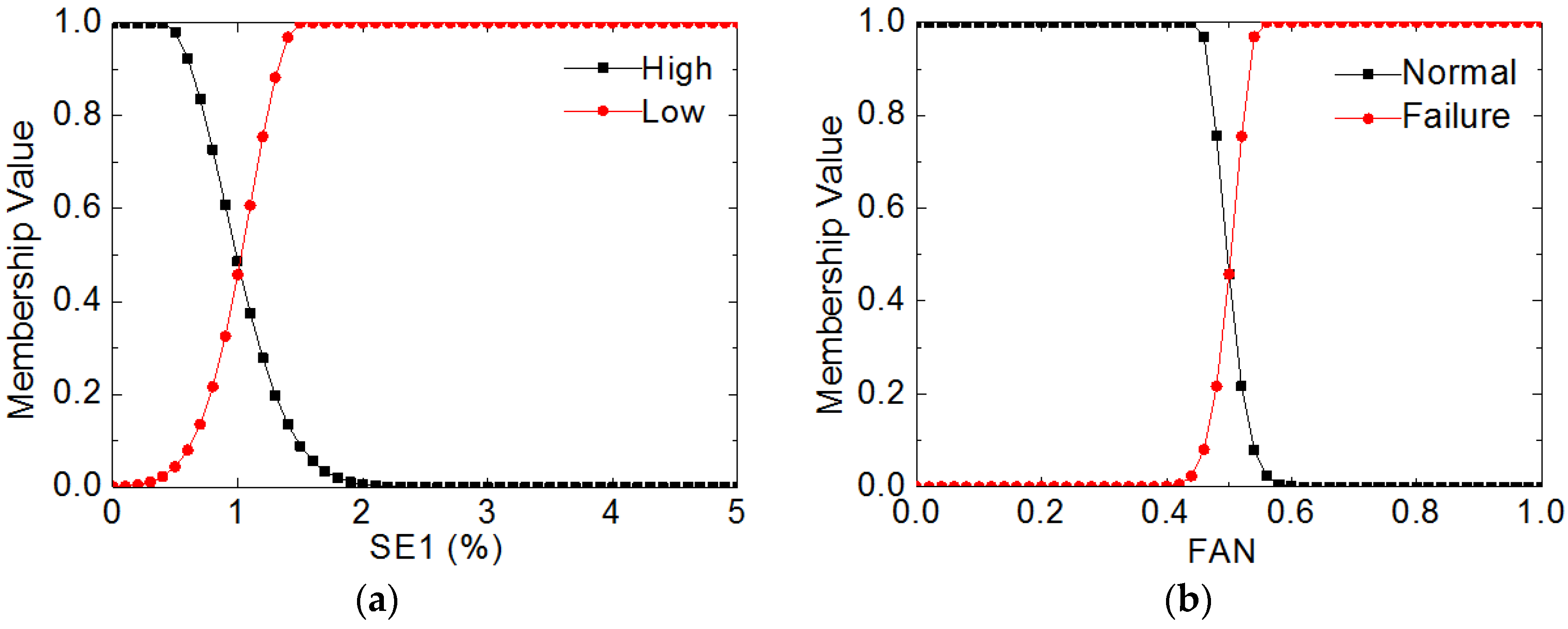
Take fuzzy logic on fan as an example, the membership functions of fault feature parameter SE1 and Fan fault mode are shown in Figure 3a,b, respectively. The membership functions for the rest fault feature parameters SE2, SE3, and SE4 and their fault modes are formulated in a similar way.
Engine performance fault classification using fuzzy logic is conducted as follows: the estimates of fault feature parameter are converted to the linguistic variables in the fuzzy subset using the Gauss membership. The linguistic variables corresponding to the outputs are obtained by the fuzzy logic rules. Fuzzy distribution is calculated in the inference machine, and the fault mode index is exactly calculated by defuzzifing. The decision of engine gas-path fault pattern is recognized using fault mode index in the feature layer, and this index is also used as the model-based evidence results for further fault diagnosis in the decision level.

3.2. Data Hierarchical Fusion Diagnosis Using Improved Weighted DS Evidence Theory

The information reasoning and fusion can be done by DS evidence theory, whereas this method might fail in some cases of information incomplete or uncertainty [43,44]. In order to improve the confidence of DS evidence theory, the WDS is developed and applied to integrate the model-based evidence E1 and data-based evidence E2 to reach a final decision of gas-path fault diagnosis. Let ϴ be an elements set of discernment frame, and it means all performance fault modes, namely, ϴ = {F1, F2, F3, F4, F5, F6, F7, F8, F9, F10}. The set map m: 2ϴ -> [0,1] is a basic probability assignment function (BPAF) in the frame ϴ, and it follows
m ( ) = 0 ; A Θ m ( A ) = 1
where the proposition A, A1, and A2 are the subsets of ϴ, is empty set, and the basic confidence m(A) is the confidence level of the proposition A. When two evidences E1 and E2 are concerned in the frame ϴ, their BPAFs are m1 and m2, respectively. The propositions A1 and A2 are corresponding to the evidences E1 and E2, and the propositions A relates to the combination of the former evidences in the frame ϴ. The BPAF of the fusion based on two evidences is expressed as follows
m ( A ) = { A 1 A 2 = A m 1 ( A 1 ) m 2 ( A 2 ) 1 K A i 0 A i =
where the parameter K = A 1 A 2 = m 1 ( A 1 ) m 2 ( A 2 ) represents the conflicts between two evidences. The inconsistence level of two evidences increases as the larger K. It has more opportunity to reach a false conclusion once the evidence conflict becomes seriously. The fault feature and fault diagnostic mechanism by the data-based and model-based evidences are different for engine gas-path system, and the WDS fusion method relies on adaptive fused BPAF of two evidences. The confusion matrix in the WDS is used to compute the confidence of each evidence, and the evidence weight in the fused BPAF is tuned to the evidence confidence.
The confusion matrices corresponding to the model-based and data-based evidences are separately expressed V1 and V2
V t = [ v 1 , 1 v 1 , 2 v 1 , 10 v 2 , 1 v 2 , 2 v 2 , 10 v 10 , 1 v 10 , 2 v 10 , 10 ] ( t = 1 , 2 ) v i , j = n i , j / n i
where ni,j is the sample number of the fault mode i misdiagnosis to fault mode j, and ni is the total sample number in fault mode i. The element vi,j is the false diagnosis percentage that the fault mode i is mis-recognized as the mode j by one evidence. The diagonal elements of the confusion matrix indicate the correct identification rate of every fault mode. In order to increase the effect of evidence that produces less incorrect recognition, the weighted coefficient is introduced
W ( A ) = k R 3 ( A ) A Θ R 3 ( A )
R ( F j ) = v j , j i = 1 10 v i , j
where the coefficient R(Fj) depicts the reliability of one evidence for fault diagnostics in the fault mode j. rank is the descending sort number of basic probability assignment in each fault mode, and smaller series number rank implies larger confidence of the evidence. k is 2 as the series number rank equals 1, 2 or 3, otherwise k is 1. The adaptive fused BPAF m*(A) is presented as follows
m * ( A ) = { A 1 A 2 = A W m 1 ( A 1 ) W m 2 ( A 2 ) 1 K A i 0 A i =
W m i ( A ) = W ( A ) m i ( A ) A Θ W ( A ) m i ( A )
where Wmi() is the weighted BPAF of the Ei, and K = A 1 A 2 = W m 1 ( A 1 ) W m 2 ( A 2 ) .
The WDS for fault diagnosis is presented in detail as follows
Step 1: Initiate the confusion matrices V1 and V2, which are calculated from training samples using Equation (25).
Step 2: Load the confusion matrices V1 and V2 to calculate the reliability parameters for two evidences using Equation (26b).
Step 3: Calculate the weighted BPAF of two evidences.
If two evidences E1 and E2 are conflicted
Calculate weighted coefficients for E1 and E2 using Equation (26a)
Calculate the weighted BPAF for E1 and E2 using Equation (27b)
Else
Wm1(A1) = m1(A1) and Wm2(A2) = m1(A2)
Step 4: Combine two evidences to reach adaptive fused BPAF using Equation (27a).
Step 5: Obtain turbofan engine gas-path fault pattern which is corresponded to the largest m*(F).
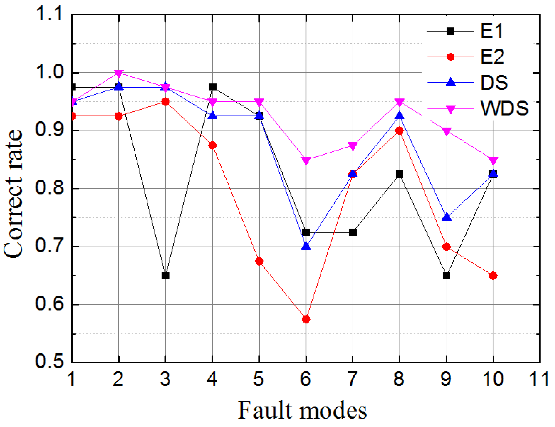
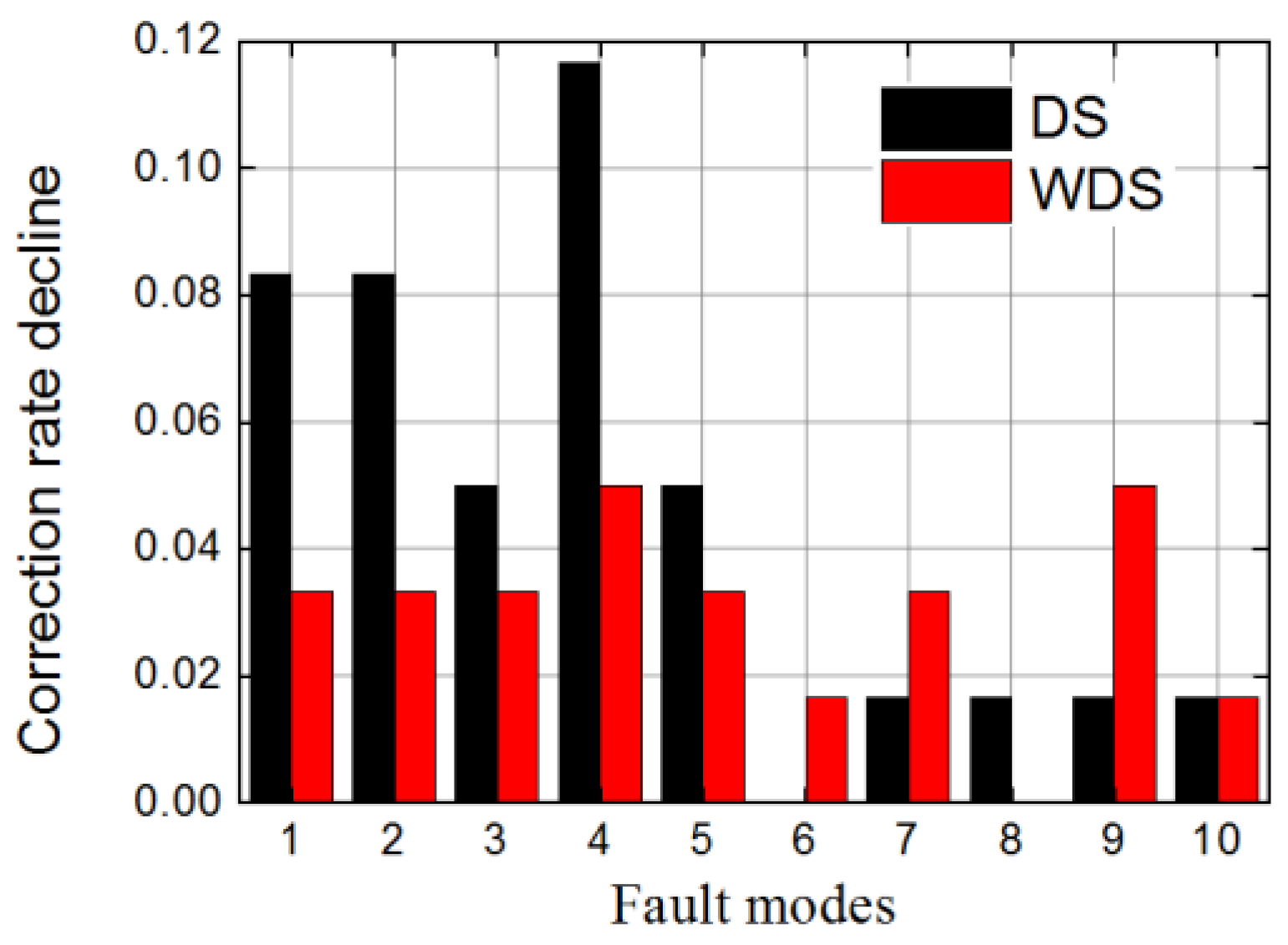
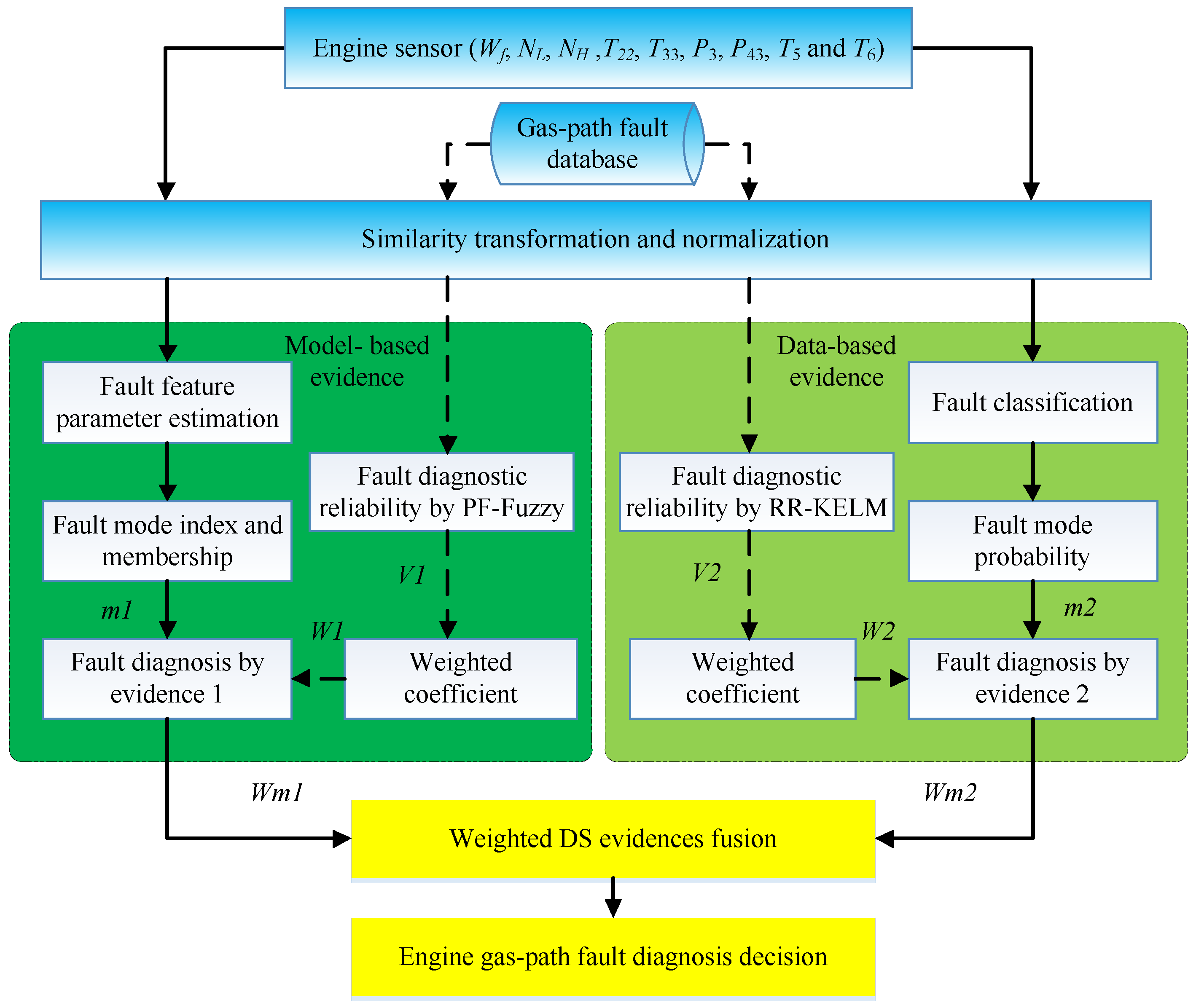
A data hierarchical fusion framework using the WDS is designed to increase the confidence of gas-path fault diagnostics for turbofan engine, and it is shown in Figure 4. The PF-FL is utilized to reach the model-based evidence for gas-path fault diagnosis, and it runs parallel with the RR-KELM in the hierarchical fusion framework. The sensed data along the engine gas path used for fault diagnosis, like speeds, temperatures, pressures, vary with the power condition and ambient conditions. In order to extend the designed approach to the whole flight envelope and decrease the negative effects of various physical parameters magnitude difference, the aero-thermodynamic parameters are corrected and normalized before the fault diagnosis applications. Details of correction and normalization can be found in Reference [36].
The engine health parameter deviations are estimated and used as fault feature parameters by fuzzy logic to produce fault mode index. Meanwhile, the RR-KELM is implemented to produce fault mode probability from the engine measurements. The confusion matrices and weighted coefficients are the prior information calculated from engine gas-path fault database. With the help of this prior information, the decisions of evidences about fault mode are obtained using the model-based and data-based methods, and then are combined to reach an engine fault pattern recognition decision by the WDS in the data hierarchical fusion framework.

4. Simulation and Analysis

The proposed gas-path fault diagnosis method is evaluated on the general gas turbine engine simulation using MATLAB software. The developed CLM of turbofan engine takes the place of an actual engine, and the sampling rate of CLM equals to 50 Hz [40,45]. The hardware of computer used for simulation is configured CPU i5-5200U @ 2.20 GHz and RAM 4 GB. The involved engine component fault patterns have been shown in Table 1, and sensor and actuator faults are not considered. Eight measurements are employed for gas-path fault diagnosis, and their standard deviations and CLM modeling errors are shown in Table 2. Gaussian noise v with standard deviations given in Table 2 is added to the measured parameters, and the independent system noise and measured noise follow w~N(0,Q) and v~N(0,R), wherein Q = 0.16 × 10⁴I6.
The training data of RR-KELM are generated by the general gas turbine simulation. The model-based method using PF-FL and data-based method using RR-KELM are separately serving as the evidence 1 (E1) and evidence 2 (E2). The comparisons of E1, E2, DS and WDS with regards to gas-path fault diagnosis confidence and robustness are carried out at typical operating points in the flight envelope.

4.1. RR-KELM Performance Test

To evaluate the classification performance of RR-KELM, benchmark datasets from UCI Machine Learning Repository are used. The attribute number (#Attribute), the number of classes (#Classes), training sample number (#Train) and testing sample number (#Test) of each dataset are listed in Table 3. The learning machine parameters for each dataset are presented in the first column in Table 4, and the best performance indices of the involved algorithms in every dataset are bolded.
All the input data are normalized into the closed span [−1, 1] and integers 1, 2, 3… are target value of different classes. The index Ac is defined by the correct classification number in the total test number, and Figure 5 shows Ac by three involved algorithms in the dataset Vehicle (Figure 5a) and dataset Satimage (Figure 5b).
As shown in Figure 5, the indices Ac by FSA-ELM and RR-KELM increases with the number of hidden nodes (#node). The dotted line can be viewed as the benchmark line generated by basic KELM. The proposed RR-KELM needs less number of hidden nodes when the testing accuracy of RR-KELM approaches to that of basic KELM. It implies the feasibility of RR-KELM to decrease the hidden nodes in benchmark datasets Vehicle and Satimage. The detailed performance comparison of the involved algorithms on classification datasets is presented in Table 4. We can find that the hidden nodes of FSA-ELM and RR-KELM reduce significantly compared to basic KELM with some loss of testing accuracy. In the most cases of benchmark datasets, especially those large scale datasets, RR-KELM performs better parsimoniousness since the constrains generated by the whole dataset are considered. That is to say, the proposed RR-KELM is superior to the rest two algorithms with regards to classification accuracy and topological structure. Therefore, the RR-KELM is used to produce the data-based evidence of performance fault diagnosis in the following tests.

4.2. Performance Comparisons at Design Operating Point on the Ground

The tests on performance of proposed data hierarchical fusion based on DS for fault diagnosis is firstly evaluated at design operation on the ground (H = 0 m, Ma = 0, Wf = 2.48 kg/s). This operating condition is denoted by Case 1. The fault mode indices calculated by PF-FL and fault probabilities by RR-KELM are used for the evidences’ BPAFs, which are integrated to produce a fused BPAF by the DS in the data hierarchical fusion architecture. The fault type is just related to the maximum element of BPAF vector. The engine health parameter changes from 0.25% to 5% with 0.25% interval to depict the magnitude of gas-path failure, and there are 20 shift amplitudes of health parameters for each fault mode. When ten fault modes plus one nominal condition are concerned, the counter of shift magnitude is 201 (10 × 20 + 1). In order to describe various engine operating points, the engine operating data related to control input from idle 0.48 kg/s to maximum power 2.48 kg/s with 0.1 kg/s interval are discussed. Consequently, there are totally 4221 (201 × 21) training samples for the RR-KELM. After 30 trials achieved with each algorithm, the best kernel parameter and particle number are selected from the empirical candidates, i.e., γ = 10, and N = 30. The BPAFs in the case of HPT fault mode (F3) by the three methods such as the E1, E2 and DS are shown in Table 5.
The largest elements of BPAFs calculated by three methods are separately 0.1784, 0.2830 and 0.3584 from Table 5, which sequentially correspond to the fault mode F10, F3 and F3. In the data hierarchical fusion framework, it means that the fault mode F10 (HPT and LPT) is identified by the E1, while F3 (HPT) by both of the E2 and DS. The correct results of fault pattern recognition are achieved by the E2 and DS, and misdiagnosis brought by the E1. It is noted that the decisions of two evidences are contradictory in this case, the final decision of fault pattern accurately brought by the DS.
The confidence to the fault mode HPT by the DS is 0.3584 and the decision of fault identification is right, but it is not large enough in the F10. To locate the gas-path fault mode more definitely, the proposed WDS is then introduced to the comparisons. As was mentioned earlier, the confusion matrix of each evidence is a key to WDS, and it is calculated at the design operating point on the ground. The samples for confusion matrices are randomly generated from fault database, and the number of samples for each fault modes is 100. Confusion matrices of model-based evidence and data-based evidence denoted by V1 and V2 are worked out using Equation (25) as follows
V 1 = [ 84 1 0 2 1 0 12 0 0 0 1 80 0 3 0 0 0 1 15 0 0 0 69 5 0 0 0 0 0 26 2 1 4 89 0 0 0 0 1 3 7 9 0 1 80 0 1 0 2 0 10 0 2 4 0 78 6 0 0 0 20 0 0 6 0 0 74 0 0 0 0 5 1 1 0 0 0 87 5 1 0 15 0 3 0 0 0 3 79 0 1 0 14 6 0 1 0 0 0 78 ] , V 2 = [ 74 2 0 7 2 2 13 0 0 0 0 65 5 1 10 2 0 8 8 1 0 4 77 0 0 6 0 8 0 5 3 2 0 81 0 0 13 0 0 1 2 3 0 0 79 9 0 0 7 0 0 3 2 0 1 87 1 0 6 0 5 0 0 11 0 2 81 0 1 0 0 9 6 0 0 1 0 83 0 1 0 8 0 0 5 1 1 0 79 6 0 0 4 0 0 6 0 1 9 80 ] .
The diagonal elements of confusion matrices V1 and V2 imply the correct number of fault diagnosis in 100 random samples for every fault mode. It is difficult to achieve fault pattern recognition without false alarm by single method PF-FL or RR-KELM for all fault patterns, and the most correct pattern recognition count from 100 samples could be completed in the fault mode F4 by the E1 and fault mode F6 by the E2. The reliability coefficients of two evidences in each fault mode then can be computed, which are presented in Table 6. These reliability coefficients varied with fault mode, and the E1 produces better fault diagnosis accuracy than the E2 in some fault modes but worse in the rest modes. For example, the R(F5) is 0.988 by the E1 while 0.814 by the E2, and R(F1) is 0.672 by the E1 less than that 0.881 by the E2. That is to say, the performance of fault diagnosis using PF-FL method is better than that using the RR-KELM method in the case F5, but it is opposite in the case F1.
In order to assess the confidence of fault diagnosis by the WDS, two engine fault modes such as HPT failure (F3) and Fan and Compressor (F5) are simulated. The fault diagnostic results by two evidences are inconsistent in the F3 as seen from Table 5, and then the weighted coefficients of evidences are computed using Equation (27b) in the data hierarchical fusion framework. The adaptive fused BPAF of the WDS is integrated based on the weighted coefficients, and Figure 6a gives the comparisons of BPAF by the basic DS and WDS approaches in the fault mode F3. We can make a more certain decision of the fault mode F3 occurrence using the WDS since the BPAF by the WDS is 0.4464 larger than that 0.3584 by the DS. The HPT failure is correctly recognized by both of the DS and WDS, but it is hard to have the satisfactory results in all cases, and the BPAFs by the DS and WDS in the fault mode F5 is shown in Figure 6b. The largest element by the WDS is m(F5) equaled to 0.336, while the maximum by the DS is m(F1) = 0.284. Hence, the faulty component by the WDS is identified as the Fan and Compressor (F5), and that by the DS is as Fan (F1). The result identified by the WDS is consistent with the real condition, but the DS provides a wrong decision.

4.3. Performance Comparisons at Typical Operating Conditions on the Ground

As was mentioned earlier, gas turbine engine operating condition is mainly defined by fuel flow, and simulations in three typical operations on the ground Case 1 (Wf = 2.48 kg/s), Case 2 (Wf = 1.98 kg/s) and Case 3 (Wf = 1.48 kg/s) are carried out. The performance comparisons of the involved methods are done in every fault mode, and the fault amplitudes of test data for the evaluation are random at three operating conditions. The performance index rp is introduced to depict correct percentage of fault pattern recognition in one fault mode
r p = i = 1 N u m m C ( F i ) N u m m × N u m s × 100 %
where the number of fault modes Numm is 10, and the count of test samples in each mode Nums is 20. The correct number of fault identification in fault mode Fi is C(Fi). Table 7 presents the performance of engine gas-path fault diagnosis by the evidences and fusion methods at three typical operations in every fault mode on the ground.
As can be seen from Table 7, the index rp decreases with the reduction of engine fuel flow by E1 since the accuracy of engine model is the best at the design operation (Case 1) and it declines as the operating point far from design point. The fault diagnosis capability by RR-KELM closely associated with the training fault sample distribution and is independent to model accuracy. Since the training samples cover from engine idle to maximum power state, the E2 has a relatively steady accuracy in three cases. The decision of fault diagnosis by the DS and WDS are integrated from the E1 and E2, the fusion methods produce better rp in the cases above, and we can also find that the performance of WDS is superior to that of DS from Table 7.
In order to compare single evidences and fusion methods in all fault modes in detail, the average of correct recognition in three cases is defined by correct rate, which is presented in Figure 7. The E1 produce better correct rate than the E2 in the former two fault modes, but worse in the remaining fault modes. The fusion method has capability of extracting the useful information of evidence to obtain a better decision. The two fusion methods have the same performances in the fault modes F1, F2, F3, F7, and F10, and the WDS performs outstanding in the rest fault modes.

4.4. Gas-Path Fault Diagnosis Test in the Flight Envelope

From the former simulations, we can see that the performance of the WDS in the data hierarchical fusion framework is better than the others for engine gas-path fault diagnosis on the ground. The robustness of the WDS in terms of full flight envelope and modeling mismatch is discussed in this section. When it comes to high altitude points in flight envelope, the proposed methodology is evaluated at the typical flight points including climbing operation H = 6000 m, Ma = 0.5, Wf = 1.28 kg/s and cruise operation H = 11,000 m, Ma = 0.8, Wf = 0.78 kg/s, separately denoted by Case 4 and Case 5. The performance comparisons of single evidences and fusion methods for gas-path fault diagnosis within flight envelope are given in Table 8.
The index rp of the E1 is 82.5% both in Case 4 and Case 5, which are relatively steady at the typical high altitude operating points. However, the rp of the E2 by the data-based evidence in Case 5 declines more compared to that in Case 4. It results from that there are not enough training data at the high altitude operating points. The E1 decision brought from the model-based evidence is closely dependent on physical thermodynamics and component map of turbofan engine. It is hardly affected by the training data as the E2, thus the E1 has a better robustness of fault diagnosis than the E2 in the flight envelope. The results calculated by the DS and WDS are closer to the true state than those by two evidences. The WDS’s rp is more than 90% in two cases above and it produces the best accuracy of fault diagnosis in Case 4 and Case 5. Ten trials are conducted for each fault scenario with every approach, and the averages of correct rate by the evidences and fusion methods in Case 4 and Case 5 are shown in Figure 8. Compared to the E1, E2 and DS, the WDS has the best correct rate except in the fault modes F1 and F4 from Figure 8. Consequently, the data hierarchical fusion based on the WDS has a satisfactory robustness at high altitude operating points in the flight envelope.

4.5. Robust Test with Modeling Uncertainty

The tests completed above are assuming that the engine model tracks actual engine well, but the modeling mismatch between the engine CLM and actual individual is inevitable in practice. The engine manufacture tolerances lead to the individual performance difference under nominal operating conditions, and the engine-to-engine variation is one of the most important reasons to cause the modeling uncertainty. The modeling uncertainty of turbofan engine can be represented by modeling errors, and it will affect the performance of model-based method. The robustness evaluation of the proposed fusion framework with regards to modeling uncertainty is performed in Case 1, Case 4 and Case 5. The modeling errors of key measurement shown in Table 2 are added to the engine CLM outputs. Fault diagnostic performance comparisons of the evidences and fusion methods with modeling uncertainty in flight envelope are given in Table 9.
The indices rp of the E1 in three cases are less than 80% when the modeling mismatch is considered, and those indices of fusion methods are also declined since one evidence accuracy decrease. While the rp of WDS both in Case 1 and Case 4 are still more than 90%, and the correct recognition number by the WDS is more than that by the DS. It indicates that the WDS has better accuracy of fault diagnostics than the DS in the cases of modeling uncertainty. In order to further present the robustness of data hierarchical fusion scheme, the correct rate average of 10 trials of three cases (Case 1, Case 4 and Case 5) in 10 fault modes are shown in Figure 9. As can be seen from Figure 9, the correct rate average of fusion methods declines as the modeling errors is injected. The DS produces more reduction of correct rate than the WDS except in three fault modes F6, F7, and F9. Besides, the maximum decline by the WDS is 0.05 while that by the DS is near 0.12. That is to say, the fluctuation by the WDS is less than that by the DS when the modeling uncertainty is considered. In a word, despite the CLM modeling mismatch of turbofan engine, the robustness of data hierarchical fusion framework based on WDS is a better candidate for gas-path fault diagnosis.

5. Conclusions

This paper develops a systematic approach including data processing and fusion mechanism which lead to an improved data hierarchical fusion framework. The novelty of this methodology lies in the development of a data fusion technique that combines sub-decisions from two different ways of fault diagnosis, namely, the model-based and data-driven methods. By computing and combining the fault mode index and fault probability of the evidences, a fused faulty index is designed to better identify gas-path failure mode for turbofan engine. Guidelines for several key elements related to the problem formulation, fault feature description, fusion scheme, fault diagnostic robustness and other important aspects are discussed and illustrated in the case study. The proposed RR-KELM algorithm brings sparseness of training data and simplifies topological structure of the learning machine, which is used to generate data-based evidence. One advantage of this methodology is that the fault pattern recognition becomes more accurate than the single evidence (the model-based or data-based one). This property could have a great impact on deciding whether to stop operation and to schedule maintenance for turbofan engine. Another advantage of this methodology is that the robustness of fault diagnosis significantly improved in terms of various operations in flight envelope and modeling uncertainty, and it implies that the data hierarchical fusion can be a more efficient tool in practice.
The methodology is validated using the faulty operating data of turbofan engine that are generated by the general gas turbine simulation. The model-based method using the PF-FL algorithm and the data-based method using the RR-KELM algorithm are served to produce fault diagnostic evidences in feature layer. It is proved that the RR-KELM is well trade-off between the classification accuracy and topology simplification. The fault mode index and fault probability related to each evidence are integrated by the fusion scheme to reach a final decision of gas-path fault diagnosis in decision layer. In the data hierarchical fusion architecture, the WDS is developed from the DS for integrating multiple evidence information with evidence reliability coefficients. The stochastic fault operating data are adopted to numerically evaluate the capability of the proposed methodology, and the performance comparisons of single and fusion methods are completed in the typical operations. In addition, the tests about modeling mismatch and lack of training data covering all fault modes are discussed in the flight envelope. Since the proposed methodology integrates the advantage of model-based and data-based methods, the confidence and robustness for gas-path fault diagnosis is expected to be improved by drawing more useful information of evidences.
This research establishes a new direction at information fusion by proposing a data hierarchical fusion technique that is specifically beneficial for engine gas-path fault diagnosis applications. There are several important topics for future research that are related to this work. First, further studies can be done to investigate the performance when engine gas-path fault feature selection and the kernel methods are used to fault feature extraction. Except for the efficiency of engine component, flow capacity could be added into fault feature parameters. Second, although this paper focuses on the engine gas-path fault diagnosis at one cycle number and no degradation considered, extensions to the cases of normal engine performance degeneration in the course of its lifetime are worthy of further exploration.

Acknowledgments

We are grateful for the financial support of the National Nature Science Foundation of China (No. 61304133), and China Outstanding Postdoctoral Science Foundation (No.2015T80552). Gratitude is also extended to Viliam Makis for useful suggestions and to China Scholarship Council for supporting the first author to carry out collaborative research in the Department of Mechanical and Industrial Engineering at the University of Toronto.

Author Contributions

Feng Lu and Jinquan Huang contributed in developing the ideas of this research. Yafan Wang, Chengxin You and Chunyu Jiang performed this research. All of the authors were involved in preparing this manuscript.

Conflicts of Interest

The authors declare no conflict of interest.

Abbreviations

The following abbreviations are used in this manuscript:
GPAGas-path analysis
NNNeural network
ELMExtreme learning machine
KFKalman filter
PFParticle filter
FLFuzzy logic
DSDempster–Shaffer evidence theory
HPTHigh pressure turbine
LPTLow pressure turbine
xState vector
yMeasured vector
hHealth parameter
wProcess noise Vector
vMeasurement noise vector
QCovariance of process noise
RCovariance of measurement noise
NLLow pressure rotor speed
NHHigh pressure rotor speed
SE1Variation of fan efficiency
SE2Variation of compressor efficiency
SE3Variation of HPT efficiency
SE4Variation of LPT efficiency
WfFuel flow rate
A 8 Nozzle area
T22Fan outlet temperature
P22Fan outlet pressure
T3Compressor outlet temperature
P3Compressor outlet pressure
T43LPT inlet temperature
T6LPT outlet temperature
rpCorrect percentage

References

  1. Volponi, A.J. Gas turbine engine health management: Past, present, and future trends. ASME J. Eng. Gas Turbines Power 2014, 136, 051201. [Google Scholar] [CrossRef]
  2. Zaidan, M.A.; Mills, A.R.; Harrison, R.F.; Fleming, P.J. Gas turbine engine prognostics using Bayesian hierarchical models: A variational approach. Mech. Syst. Signal Process. 2016, 70–71, 120–140. [Google Scholar] [CrossRef]
  3. Lamaris, V.T.; Hountalas, D.T. A general purpose diagnostic technique for marine diesel engines—Application on the main propulsion and auxiliary diesel units of a marine vessel. Energy Convers. Manag. 2010, 51, 740–753. [Google Scholar] [CrossRef]
  4. Kraft, J.; Sethi, V.; Singh, R. Optimization of aero gas turbine maintenance using advanced simulation and diagnostic methods. ASME J. Eng. Gas Turbines Power 2014, 136, 111601. [Google Scholar] [CrossRef]
  5. Zhang, X.D.; Tang, L.; Decastro, J.A. Robust fault diagnosis of aircraft engines: A nonlinear adaptive estimation-based approach. IEEE Trans. Control Syst. Technol. 2013, 21, 861–868. [Google Scholar]
  6. Li, Y.G.; Korakianitis, T. Nonlinear weighted-least-squares estimation approach for gas-turbine diagnostic applications. J. Propuls. Power 2011, 27, 337–345. [Google Scholar] [CrossRef]
  7. Simon, D.L.; Armstrong, J.B. An integrated approach for aircraft engine performance estimation and fault diagnostics. ASME J. Eng. Gas Turbines Power 2013, 135, 071203. [Google Scholar] [CrossRef]
  8. Pourbabaee, B.; Meskin, N.; Khorasani, K. Sensor fault detection, isolation, and identification using multiple-model-based hybrid Kalman filter for gas turbine engines. IEEE Trans. Control Syst. Technol. 2015, 24. [Google Scholar] [CrossRef]
  9. Lu, F.; Huang, J.Q.; Lv, Y.Q. Gas path health monitoring for a turbofan engine based on a nonlinear filtering approach. Energies 2013, 6, 492–513. [Google Scholar] [CrossRef]
  10. Simon, D. A comparison of filtering approaches for aircraft engine health estimation. Aerosp. Sci. Technol. 2008, 12, 276–284. [Google Scholar] [CrossRef]
  11. Borguet, S.; Léonard, O. Comparison of adaptive filters for gas turbine performance monitoring. J. Comput. Appl. Math. 2010, 234, 2202–2212. [Google Scholar] [CrossRef]
  12. Barelli, L.; Bidini, G.; Bonucci, F. Diagnosis of a turbocharging system of 1 MW internal combustion engine. Energy Convers. Manag. 2013, 68, 23–39. [Google Scholar] [CrossRef]
  13. Bettocchi, R.; Pinelli, M.; Spina, P.R.; Venturini, M. Artificial intelligence for the diagnostics of gas turbines-part 2: Neuro-fuzzy approach. ASME J. Eng. Gas Turbines Power 2006, 129, 720–729. [Google Scholar] [CrossRef]
  14. Sampath, S.; Singh, R. An integrated fault diagnostics model using genetic algorithm and neural networks. ASME J. Eng. Gas Turbines Power 2006, 128, 49–56. [Google Scholar] [CrossRef]
  15. Tayarani-Bathaie, S.S.; Khorasani, K. Fault detection and isolation of gas turbine engines using a bank of neural networks. J. Process Control 2015, 36, 22–41. [Google Scholar] [CrossRef]
  16. Mohammadi, E.; Montazeri-Gh, M. Performance enhancement of global optimization-based gas turbine fault diagnosis systems. J. Propuls. Power 2016, 32, 214–224. [Google Scholar] [CrossRef]
  17. Urban, L.A. Gas Turbine Engine Parameter Interrelationships, 2nd ed.; Hamilton Standard Division of United Aircraft Corp. (HSDUTC): Windsor Locks, CT, USA, 1969. [Google Scholar]
  18. Lu, F.; Wang, Y.F.; Huang, J.Q.; Huang, Y.H. Gas turbine transient performance tracking using data fusion based on an adaptive particle filter. Energies 2015, 8, 13911–13927. [Google Scholar] [CrossRef]
  19. Hanachi, H.; Liu, J.; Banerjee, A.; Chen, Y. Sequential state estimation of nonlinear/non-Gaussian systems with stochastic input for turbine degradation estimation. Mech. Syst. Signal Process. 2016, 72–73, 32–45. [Google Scholar] [CrossRef]
  20. Decastro, J.A.; Frederick, D.K.; Tang, L. Engine Parameter Estimation in Test Cells Using Hybrid Physics/Empirical Models; ASME Paper No. GT2011-45633; ASME: New York, NY, USA, 2011. [Google Scholar]
  21. Pourbabaee, B.; Meskin, N.; Khorasani, K. Robust sensor fault detection and isolation of gas turbine engines subjected to time-varying parameter uncertainties. Mech. Syst. Signal Process. 2016, 76–77, 136–156. [Google Scholar] [CrossRef]
  22. Amozegar, M.; Khorasani, K. An ensemble of dynamic neural network identifiers for fault detection and isolation of gas turbine engines. Neural Netw. 2016, 76, 106–121. [Google Scholar] [CrossRef] [PubMed]
  23. Barad, S.G.; Ramaiah, P.V.; Giridhar, R.K.; Krishnaiah, G. Neural network approach for a combined performance and mechanical health monitoring of a gas turbine engine. Mech. Syst. Signal Process. 2012, 27, 729–742. [Google Scholar] [CrossRef]
  24. Cortes, C.; Vapnik, V. Support-vector network. Mach. Learn. 1995, 20, 273–297. [Google Scholar] [CrossRef]
  25. Fei, S.W. A hybrid model of EMD and multiple-kernel RVR algorithm for wind speed prediction. Int. J. Electr. Power Energy Syst. 2016, 78, 910–915. [Google Scholar] [CrossRef]
  26. Zhou, D.J.; Zhang, H.S.; Weng, S.L. A new gas path fault diagnostic method of gas turbine based on support vector machine. ASME J. Eng. Gas Turbines Power 2015, 137, 102605. [Google Scholar] [CrossRef]
  27. Huang, G.B.; Zhou, H.M.; Ding, X.J.; Zhang, R. Extreme learning machine for regression and multiclass classification. IEEE Trans. Syst. Man Cybern. 2012, 42, 513–529. [Google Scholar] [CrossRef] [PubMed]
  28. Yang, Y.M.; Wang, Y.N.; Yuan, X.F. Bidirectional extreme learning machine for regression problem and its learning effectiveness. IEEE Trans. Neural Netw. Learn/Syst. 2012, 23, 1498–1505. [Google Scholar] [CrossRef] [PubMed]
  29. Luo, J.; Vong, C.M.; Wong, P.K. Sparse Bayesian extreme learning machine for multi-classification. IEEE Trans. Neural Netw. Learn. Syst. 2014, 25, 836–843. [Google Scholar] [PubMed]
  30. Bai, Z.; Huang, G.B.; Wang, D.W.; Wang, H.; Westover, M.B. Sparse extreme learning machine for classification. IEEE Trans. Cybern. 2014, 44, 1858–1870. [Google Scholar] [CrossRef] [PubMed]
  31. Li, X.; Mao, W.; Jiang, W. Fast sparse approximation of extreme learning machine. Neurocomputing 2014, 128, 96–103. [Google Scholar] [CrossRef]
  32. Liu, K.; Gebraeel, N.Z.; Shi, J. A data-level fusion model for developing composite health indices for degradation modeling and prognostic analysis. IEEE Trans. Autom. Sci. Eng. 2013, 10, 652–664. [Google Scholar] [CrossRef]
  33. Kyriazis, A.; Mathioudakis, K. Gas turbine fault diagnosis using fuzzy-based decision fusion. J. Propuls. Power 2009, 25, 335–343. [Google Scholar] [CrossRef]
  34. Butler, S.W.; Pattipati, K.R.; Volponi, A.; Hull, J.; Rajamani, R.; Siegel, J. An Assessment Methodology for Data-Driven and Model-Based Techniques for Engine Health Monitoring; American Society of Mechanical Engineers (ASME): New York, NY, USA, 2006. [Google Scholar]
  35. Chacartegui, R.; Sanchez, D.; Munoz, A.; Sanchez, T. Real Time Simulation of Medium Size Gas Turbines. Energy Convers. Manag. 2011, 52, 713–724. [Google Scholar] [CrossRef]
  36. Sun, J.G.; Vasilyev, V.; Ilyasov, B. Advanced Multivariable Control Systems of Aeroengines; Beihang Press: Beijing, China, 2005; pp. 60–108. [Google Scholar]
  37. Chen, H.L.; Wang, G.; Ma, C.; Cai, Z.N.; Liu, W.B.; Wang, S.J. An efficient hybrid kernel extreme learning machine approach for early diagnosis of Parkinson’s disease. Neurocomputing 2016, 184, 131–144. [Google Scholar] [CrossRef]
  38. Subrahmanya, N.; Shin, Y.C.; Meckl, P.H. A Bayesian machine learning method for sensor selection and fusion with application to on-board fault diagnostics. Mech. Syst. Signal Process. 2010, 24, 182–192. [Google Scholar] [CrossRef]
  39. Basir, O.; Yuan, X. Engine fault diagnosis based on multi-sensor information fusion using dempster-shafer evidence theory. Inform. Fusion 2007, 8, 379–386. [Google Scholar] [CrossRef]
  40. Zhou, W.X. Research on Object-Oriented Modeling and Simulation for Aeroengine and Control System. Ph.D. Thesis, Nanjing University of Aeronautics and Astronautics, Nanjing, Jiangsu, China, 2007. [Google Scholar]
  41. Gordon, N.; Salmond, D.; Smith, A. Novel approach to nonlinear/non-Gaussian bayesian state estimation. IEE Proc. F Radar Signal Process 1993, 140, 107–113. [Google Scholar] [CrossRef]
  42. Aditya, K.; Daniel, V. Model-Based Fault Tolerant Control; National Aeronautics and Space Administration (NASA): Greenbelt, MD, USA, 2008. [Google Scholar]
  43. Jousselme, A.L.; Maupin, P. Distances in Evidence theory: Comprehensive survey and generalizations. Int. J. Approx. Reason. 2012, 53, 118–145. [Google Scholar] [CrossRef]
  44. Deng, X.; Liu, Q.; Deng, Y.; Mahadevan, S. An improved method to construct basic probability assignment based on the confusion matrix for classification problem. Inform. Sci. 2016, 340, 250–261. [Google Scholar] [CrossRef]
  45. Lu, F.; Zheng, W.H.; Huang, J.Q.; Feng, M. Life cycle performance estimation and in-flight health monitoring for gas turbine engine. ASME J. Dyn. Syst. Meas. Control 2016, 138, 091009. [Google Scholar] [CrossRef]
Figure 1. A model-based method for gas turbine engine health monitoring.
Energies 09 00828 g001
Figure 2. Schematic representation of gas turbine engine.
Energies 09 00828 g002
Figure 3. (a) Membership function for SE1; and (b) membership function for fan fault mode.
Energies 09 00828 g003
Figure 4. Data hierarchical fusion framework for engine gas-path fault diagnosis.
Energies 09 00828 g004
Figure 5. Testing results on classification datasets: (a) Vehicle; and (b) Satimage.
Energies 09 00828 g005
Figure 6. The comparisons of DS and WDS in the fault modes of HPT and Fan and Compressor: (a) fault mode of HPT; and (b) fault mode of Fan and Compressor.
Energies 09 00828 g006
Figure 7. Correct rate comparisons of the single and fusion methods in the typical operations on the ground.
Energies 09 00828 g007
Figure 8. Correction rate average comparisons of evidence and fusion methods in the flight envelope.
Energies 09 00828 g008
Figure 9. Correct rate average declines of fusion methods with modeling uncertainty in flight envelope.
Energies 09 00828 g009
Table 1. Fuzzy logic rules for engine gas-path fault diagnosis.
Rule No.IfThenFault Component
ΔSE1ΔSE2ΔSE3ΔSE4Fault Mode
1HighLowLowLowF1Fan
2LowHighLowLowF2Compressor
3LowLowHighLowF3HPT
4LowLowLowHighF4LPT
5HighHighLowLowF5Fan and Compressor
6HighLowHighLowF6Fan and HPT
7HighLowLowHighF7Fan and LPT
8LowHighHighLowF8Compressor and HPT
9LowHighLowHighF9Compressor and LPT
10LowLowHighHighF10HPT and LPT
Table 2. Gas turbine engine measurement numerical characteristics.
MeasurementAcronymsNominal ValueStandard DeviationModeling Errors
Low pressure spool speedNL10.00750.0015
High pressure spool speedNH10.00750.0015
Fan outlet temperatureT2210.01000.0020
Fan outlet pressureP2210.00750.0015
Compressor outlet temperatureT310.01000.0020
Compressor outlet pressureP310.00750.0015
HPT outlet temperatureT4310.01000.0020
LPT outlet temperatureT610.01000.0020
Table 3. Specification of classification datasets.
Dataset#Attribute#Classes#Train#Test
Iris4310050
Wine13312058
Vehicle184600246
Segment1971600710
Satimage36644352000
Page10540001473
USPS2561072912007
Letter1626150002000
Table 4. Performance comparison of KELM, FSA-ELM, and RR-KELM on classification datasets.
DatasetAlgorithmAc (%)trTime (s)teTime (ms)#node
Iris C = 10 3 , γ = 2 5 KELM960.0675.23100
FSA-ELM880.0380.2410
RR-KELM960.0080.2610
Wine C = 10 3 , γ = 2 5 KELM72.410.0030.44120
FSA-ELM70.690.0210.5640
RR-KELM72.410.0090.2420
Vehicle C = 10 2 , γ = 2 3 KELM84.510.0269.3600
FSA-ELM82.521.5161.82160
RR-KELM84.551.571.78160
Segment C = 10 3 , γ = 2 2 KELM96.760.30671.021600
FSA-ELM95.294.3138.14160
RR-KELM96.068.8138.32160
Paper C = 10 2 , γ = 2 3 KELM94.374.411292.924000
FSA-ELM89.8872.8145.54640
RR-KELM92.3274.08817.27160
Satimage C = 10 1 , γ = 2 2 KELM91.252.953453.054435
FSA-ELM89.391.48575.04640
RR-KELM90.4175.00748.91320
USPS C = 10 3 , γ = 2 5 KELM96.4113.2571284.67291
FSA-ELM93.8798.23280.5320
RR-KELM94.322218.353160
Letter C = 10 1 , γ = 2 4 KELM89.4229.841593.2815000
FSA-ELM86.23192.5105.72640
RR-KELM88.53436.5668.63320
Table 5. The BPAFs comparisons of three involved methods in the fault mode F3 at design operation on the ground.
Methodm(F1)m(F2)m(F3)m(F4)m(F5)m(F6)m(F7)m(F8)m(F9)m(F10)
E10.08360.08370.14740.08490.08360.08380.08360.08720.08370.1784
E20.04600.04490.28300.05410.08800.06500.08300.15930.02830.1485
DS0.03300.03220.35840.03950.06320.04670.05960.11930.02030.2276
Table 6. Reliability coefficients of ten fault modes by evidence.
MethodR(F1)R(F2)R(F3)R(F4)R(F5)R(F6)R(F7)R(F8)R(F9)R(F10)
E10.6720.7210.7670.7420.9880.9870.7960.9560.7750.722
E20.8810.6770.8190.8100.8140.7500.7430.8300.7180.851
Table 7. Fault diagnostic performance comparisons of the involved methods in the typical operations on the ground.
ScenarioMethodC(F1)C(F2)C(F3)C(F4)C(F5)C(F6)C(F7)C(F8)C(F9)C(F10)rp (%)
Case 1E11919151817181915191788.0
E21717162018192015201588.5
DS2019172018192018201995.0
WDS2019182020192019201997.0
Case 2E11618161916171617171684.0
E21317181818181717161885.0
DS1619181919181918171890.5
WDS1718182020181819171891.5
Case 3E11819141918161516171483.0
E21916191818151716191586.0
DS2019201918171618181690.5
WDS1920192020181719191693.5
Table 8. Performance comparisons for fault diagnosis in the typical high altitude operating points.
ScenarioMethodC(F1)C(F2)C(F3)C(F4)C(F5)C(F6)C(F7)C(F8)C(F9)C(F10)rp (%)
Case 4E11919132019161515121782.5
E21918191912131718171483.0
DS1919192019141718151889.0
WDS1920202019171819171893.5
Case 5E12020131918131418141682.5
E21819191615101618111277.0
DS1920201718141619151586.5
WDS1920191819171719191691.5
Table 9. Fault diagnostic performance comparisons of the involved methods with modeling uncertainty.
ScenarioMethodC(F1)C(F2)C(F3)C(F4)C(F5)C(F6)C(F7)C(F8)C(F9)C(F10)rp (%)
Case 1E11710121519181517131977.5
E21717162018192015201588.5
DS1619171918182017191991.0
WDS1820182019192018181994.5
Case 4E114871016171117101864.0
E21918191912131718171483.0
DS1916171718151718181786.0
WDS1918181919181719171891.0
Case 5E111810914161119161966.5
E21819191615101618111277.0
DS1818191416141619161582.5
WDS1919191618151620181588.0

