
Development of an Axial Flux MEMS BLDC Micromotor with Increased Efficiency and Power Density

Abstract
:1. Introduction
2. Basic Structure and Operation Principle
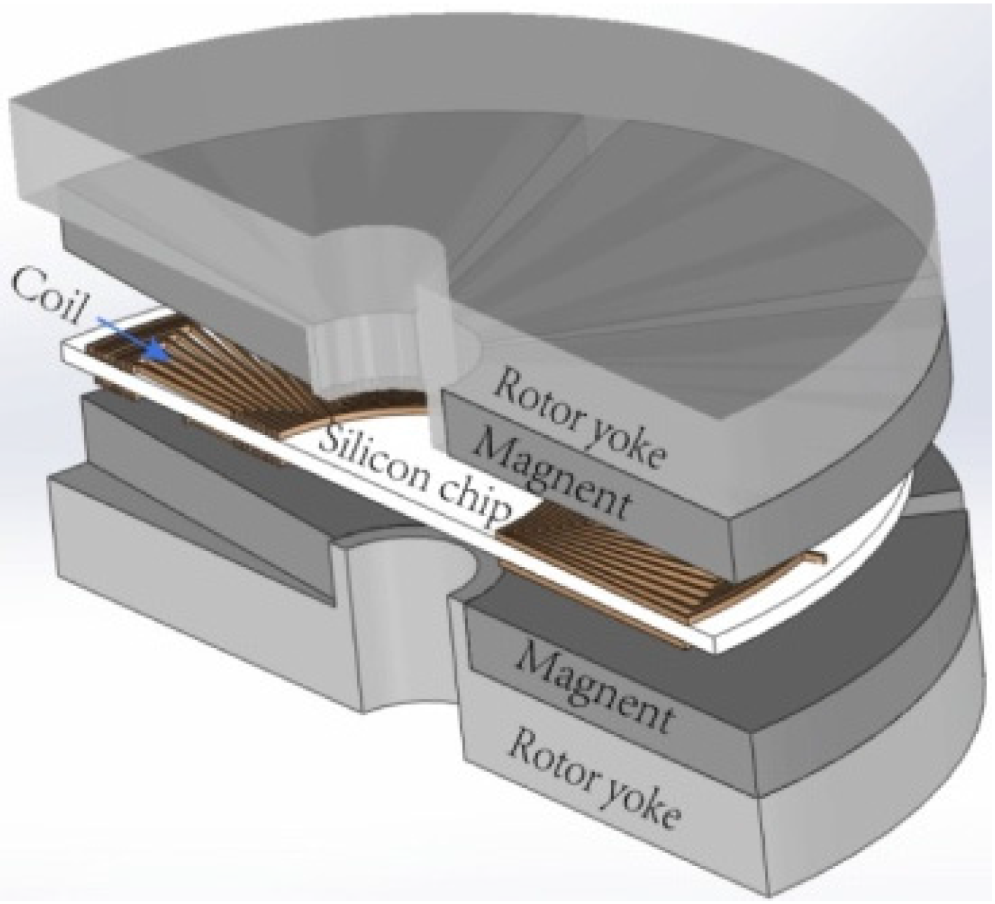
2.1. The Micromotor Structure

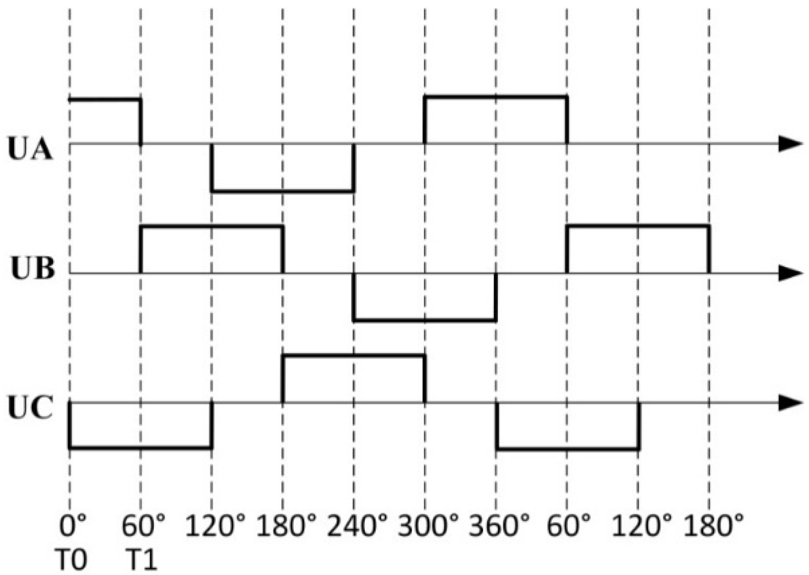
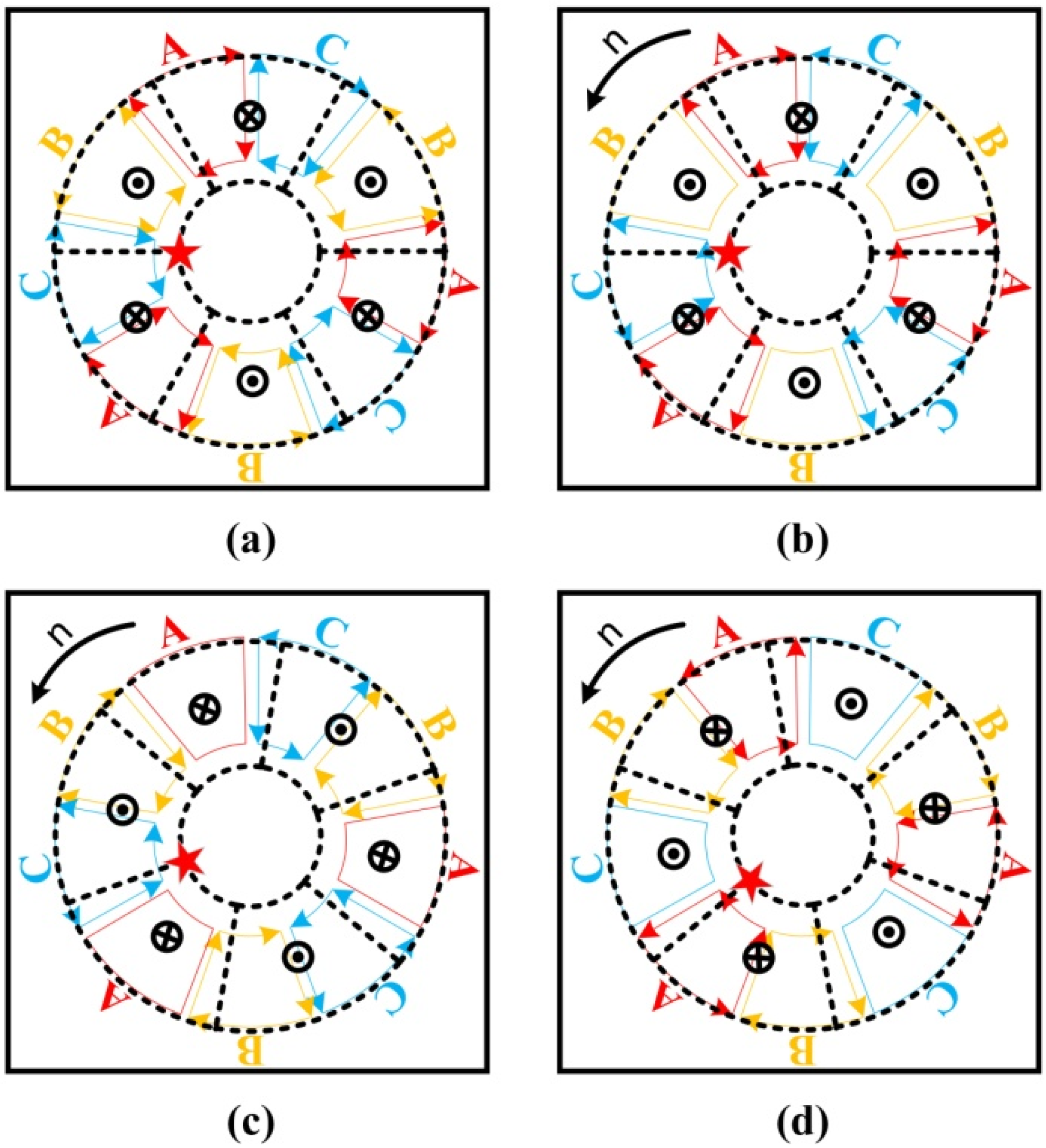
2.2. Operation Principle

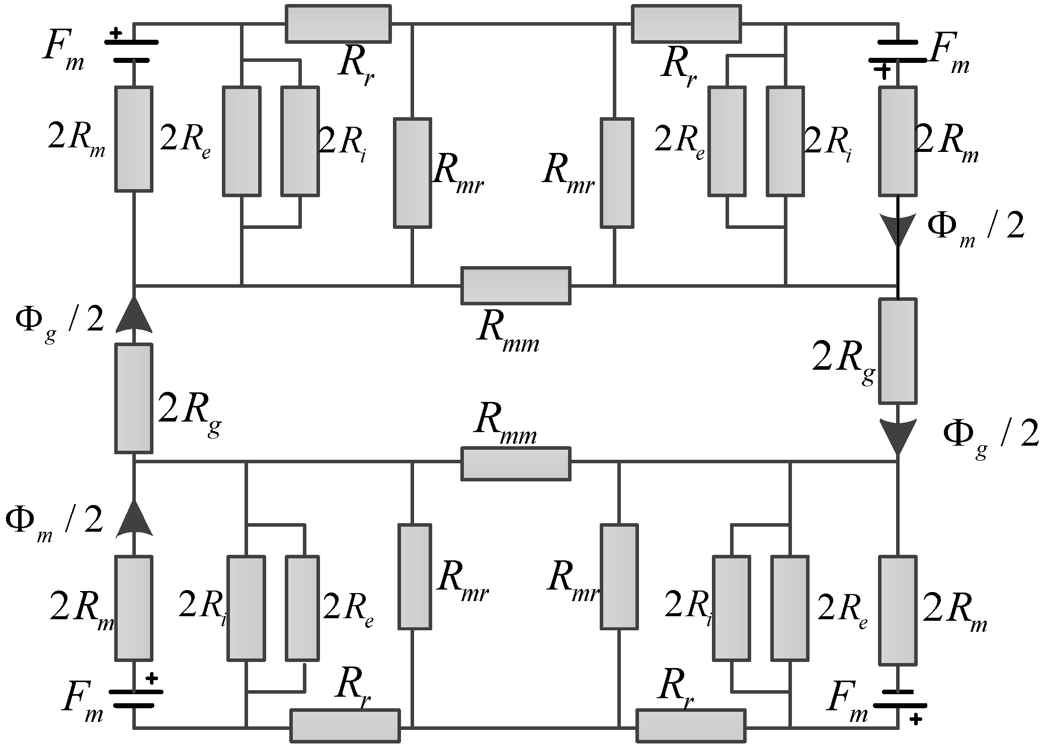
3. Analytical Modeling
- There is no saturation occurring in the rotor yokes;
- The magnetic field intensity produced by the armature current in the stator windings is negligible;
- The reluctances of the rotor yokes are neglected.
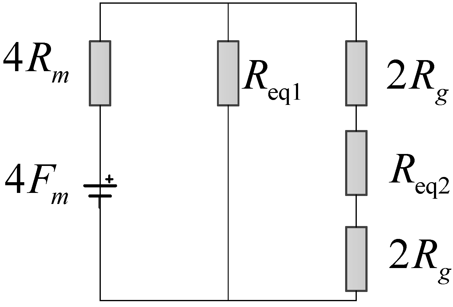
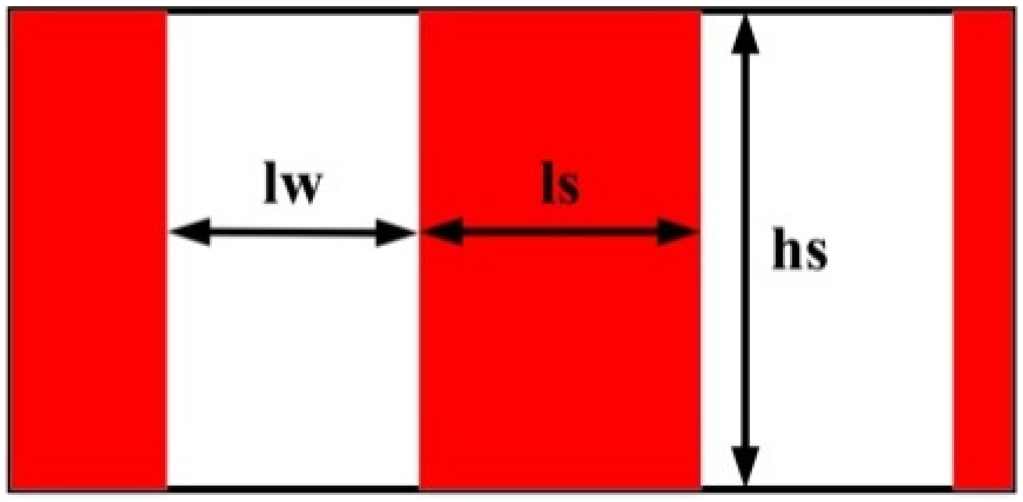
3.1. Flux Density in Air Gap


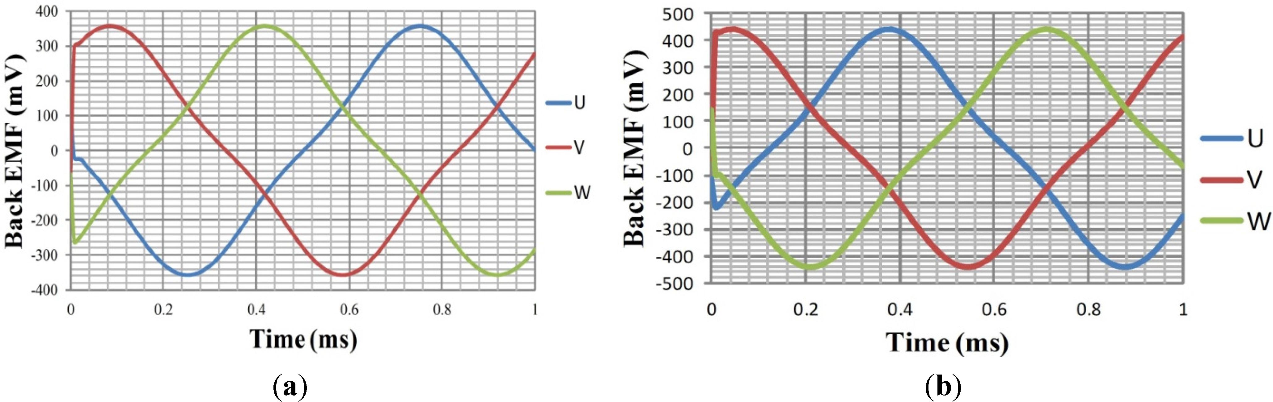
3.2. Back EMF
- back EMF of conductor i;
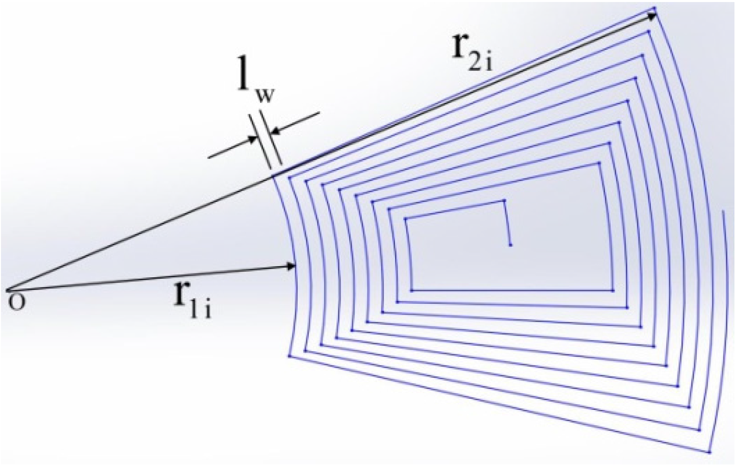
- internal radius of turn i;
- external radius of turn i;
- the electrical angle of conductor i;
- i =0,1,2,3…k-1;
- k the number of turns in one coil;
- rotation angle velocity.

- k the number of turns in one coil;
- radian of one coil;
- P number of pole pairs;
- n number of coils on one side of silicon wafer;
- ;
- insulator width;
- external radius of coil;
- internal radius of coil.
3.3. Average Output Torque
3.4. Joule Efficiency of Motor
4. Model Validation by FEA Simulations and Experiments


| Parameter | Symbol | Value |
|---|---|---|
| Rated current (A) | 0.1 | |
| Rated speed (rpm) | n | 20,000 |
| Stator external diameter (mm) | 9.5 | |
| Stator internal diameter (mm) | 2.5 | |
| Magnet height (mm) | 0.75 | |
| Magnet pole arc ratio | - | 0.85 |
| Rotor back iron height (mm) | 1.5 | |
| Air-gap length (mm) | 1.6 | |
| Pole pairs | p | 3 |

| Physical Variable | Analytical Model | FEA | Experiment |
|---|---|---|---|
| Flux density, | 0.5797 | 0.59 | - |
| Torque, | 9.68 | 9.89 | 10.25 |
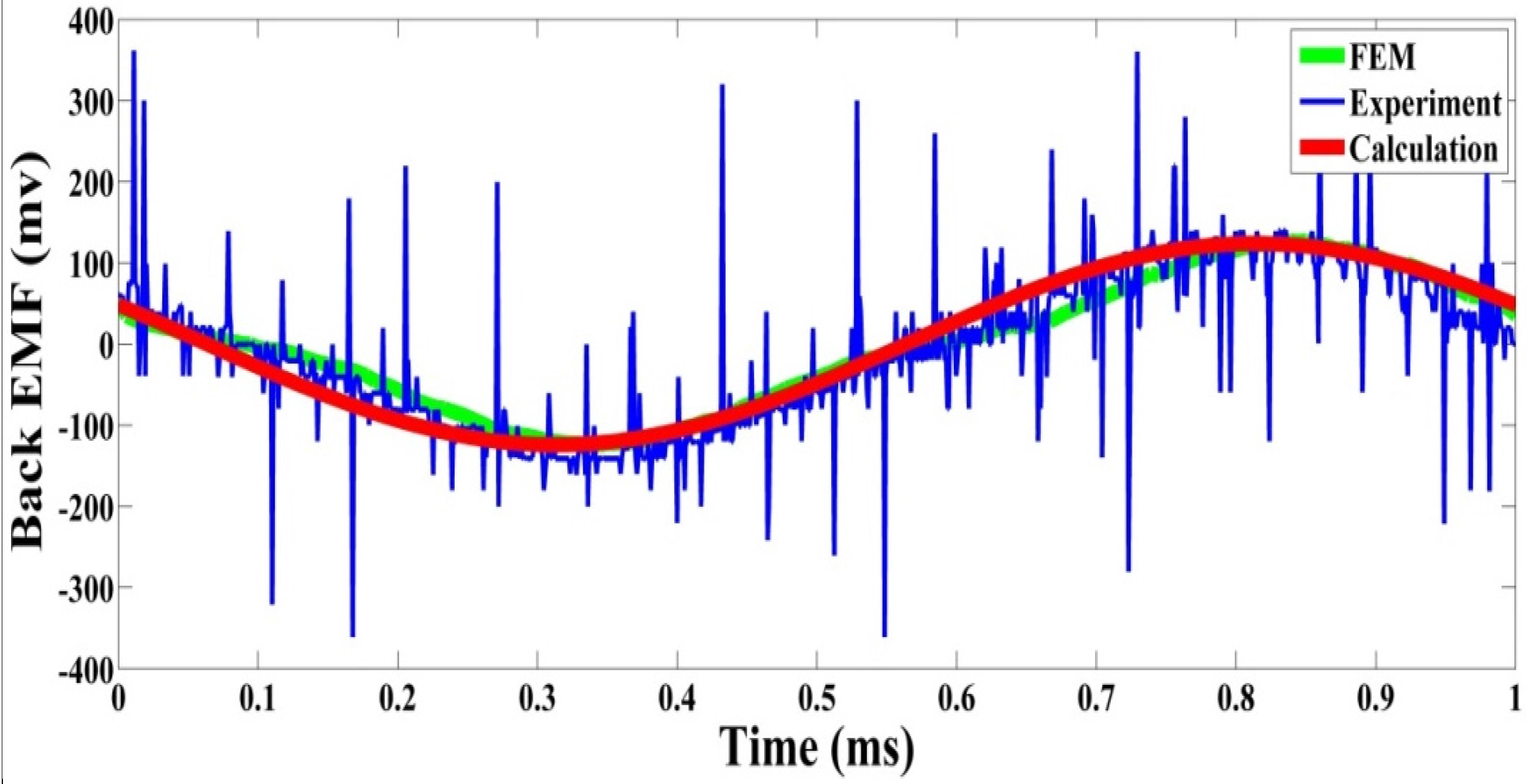
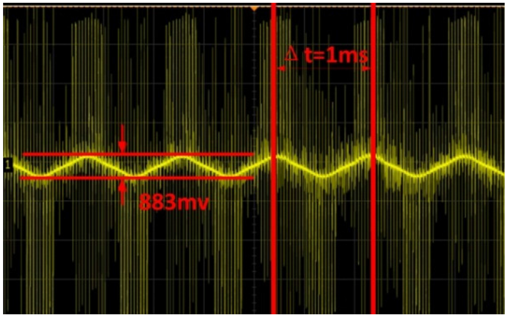
| Back EMF, | 122 | 128 | 130.5 |
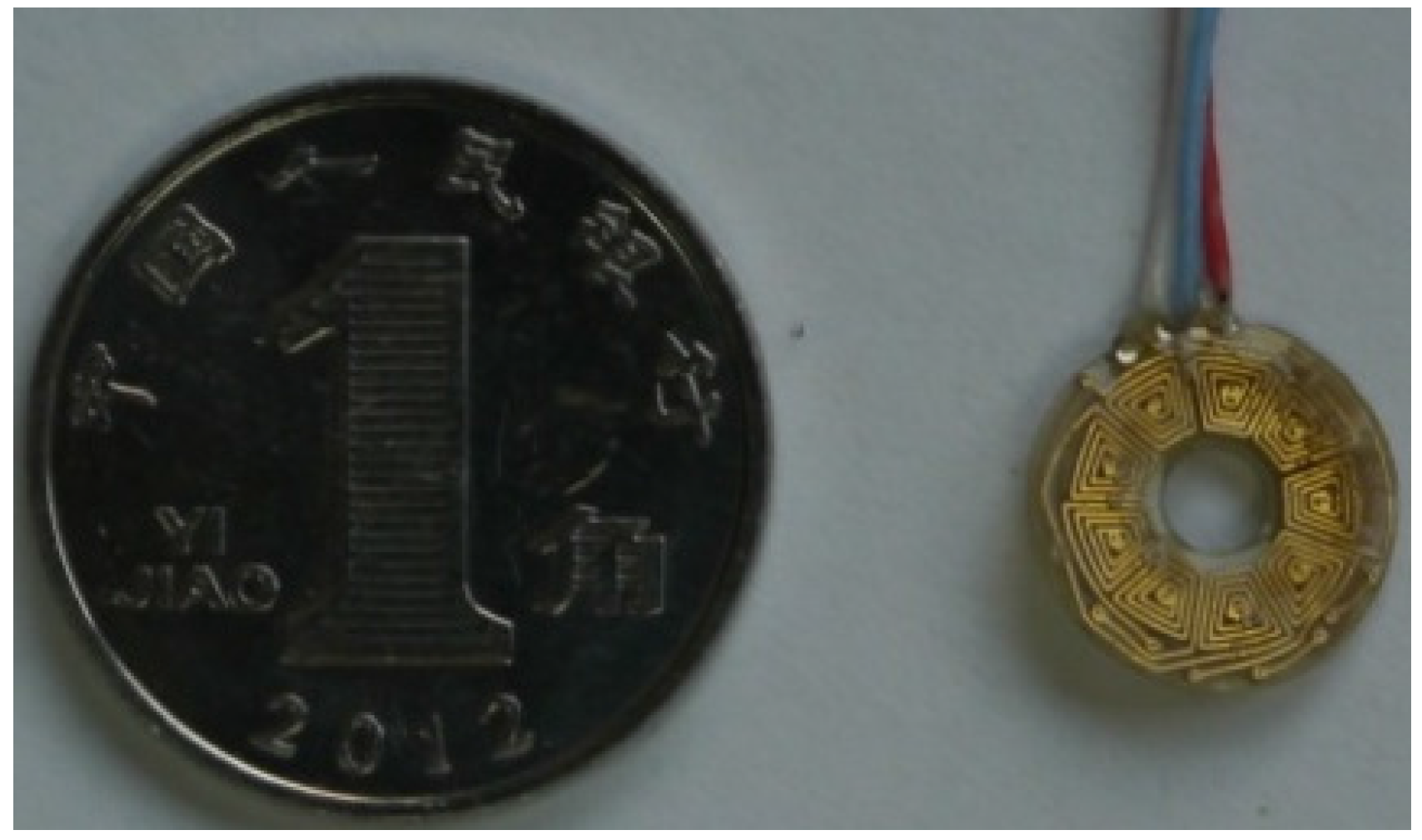
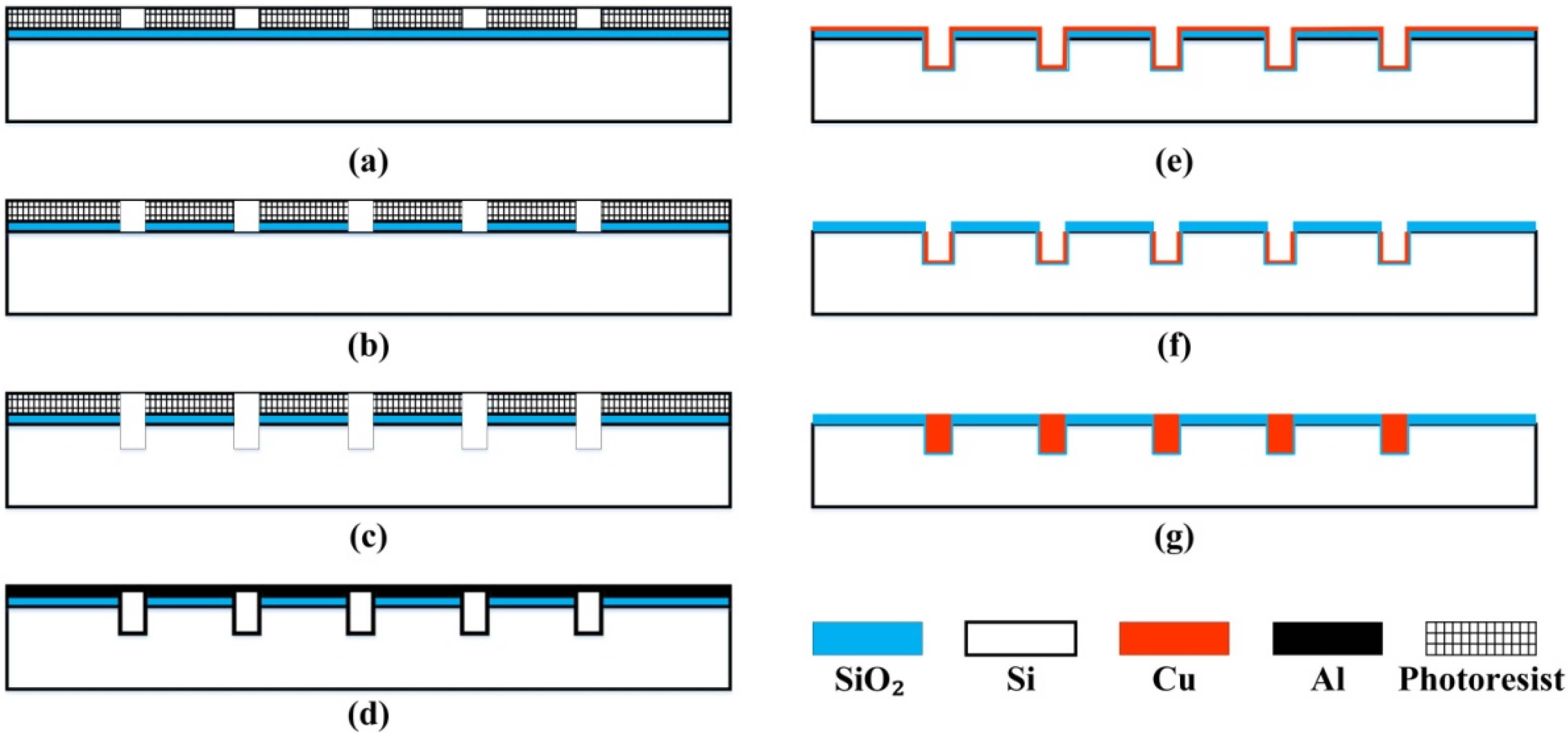
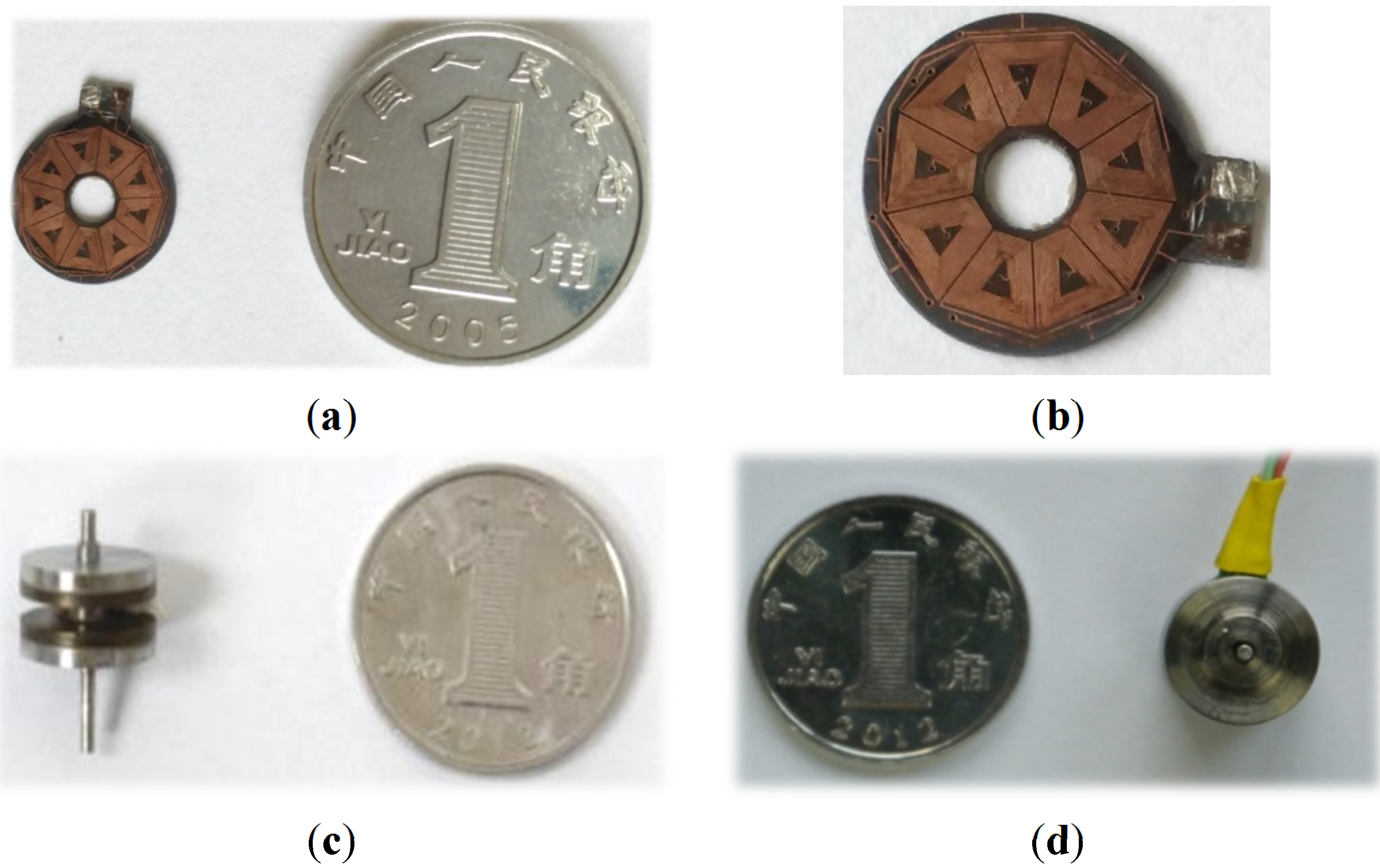
5. Stator Fabrication
| Parameters | PCB | MEMS |
|---|---|---|
| Min width of conductor | 0.1 mm | Less than 10 μm |
| Max height of conductor | 0.1 mm | More than 80 μm |
| Insulator | 0.1 mm | Less than 10 μm |
- Step 1:
- The fabrication starts from a silicon wafer with thickness of 400 μm and a 4 μm silicon oxide (SiO2) layer. Then spin coating, prebaking, exposure and development of the silicon wafer are implemented in sequence (Figure 12a). The prebaking temperature affects the exposure and development performances directly, so a suitable temperature of 115 °C is selected based on the experimental results;
- Step 2:
- The silicon wafer is baked via a hot plate. The exposed SiO2 layer is etched off via hydrofluoric (HF) acid (Figure 12b);
- Step 3:
- Grooves with width of 42 μm and depth of 80 μm are etched on the slicon wafer by an ALCATEL601E inductively coupled plasma etcher (ICP) (Figure 12c). Photoresist and SiO2 are used as a hard mask;
- Step 4:
- A 1 μm aluminum (Al) layer is sputtered over the upper surface of the silicon wafer. Then spin coating, exposure, development and etch are carried out on this surface. The holes are etched in the ICP again after stripping of photoresist (Figure 12d) Al is used to protect the upper surface of the silicon wafer while the down surface is in the fabrication stage. The fabrication process of the down surface is the same as the upper side, therefore only the upper side process is described;
- Step 5:
- A complete silicon groove structure is formed after removing the aluminum cover. After a wet oxidation of the grooves to prevent any short circuits via the silicon substrate, a copper (Cu) seed layer with 200 nm thickness is sputtered over the whole wafer surface (Figure 12e);
- Step 6:
- After a second photolithography and etch, only the cooper seed layer in the grooves is left (Figure 12f);
- Step 7:
- Finally these grooves are filled with the electroplated copper to create the metal lines of the windings (Figure 12g).

6. Firefly Algorithm-Based Design Optimization
| Variables | Range | Unit |
|---|---|---|
| Stator external diameter | [6~15] | mm |
| Magnet height | [0.5~2.2] | mm |
| Number of coils | [6~15] | |
| Conductor width | [0.04~0.06] | mm |
| Insulator width | [0.02~0.04] | mm |
| Power voltage | [1~1.5] | V |
| Variables | Value | Unit |
|---|---|---|
| Rated current | ≤0.1 | A |
| Rated speed | 20,000 | rpm |
| Pole pairs | 3 | |
| Torque | >35 | |
| Air-gap length (mm) | 1.5 | mm |
| Stator internal diameter (mm) | 3 | mm |
- Step 1:
- Initialize the numbers of fireflies n, biggest attraction , absorption coefficient of light intensity , step size factor α, and maximum of iterations or generations .
- Step 2:
- Initialize the positions of fireflies randomly, namely initializing design variables of the machine, the values of objective functions of fireflies are set as their maximum brightness of fluorescence .
- Step 3:
- Calculate relative brightness and attractiveness of fireflies, which belong to the population. The direction of movement depends on the relative brightness of fireflies. Here:where I0 is the maximum fluorescence brightness of the firefly, namely the fluorescence brightness itself (r = 0), which depends on the value of the objective function. β0 is the maximum attractiveness, namely the attractiveness of the light source (r = 0). γ is the absorption coefficient of the light intensity. The fluorescence will gradually weaken according to the increasing distance and the absorption of media. The absorption coefficient of light intensity is set to reflect this feature. is the spatial distance between firefly i and j.
- Step 4:
- Update the spatial positions of fireflies. Random perturbations are injected to the firefly with the best position. The updated equation is:where represent the spatial positions of firefly i and j, respectively. α is step size factor. rand is random factor distributed uniformly in [0,1].
- Step 5:
- Recalculate the brightness of fireflies according to the updated positions.
- Step 6:
- Return to Step 3 until the search precision is met or the maximum number of generations is achieved.
| Variables Comparison | Reference | MOFA |
| Number of coils | 9 | 9 |
| Stator external diameter ( | 9.6 | 10.2 |
| PM thickness | 0.8 | 0.88 |
| Insulator width ( | 0.04 | 0.042 |
| Conductor width ( | 0.04 | 0.038 |
| Power voltage (V) | 1.26 | 1.5 |
| Performance Comparison | Reference | MOFA |
| Dimension | 367.43 | 439.12 |
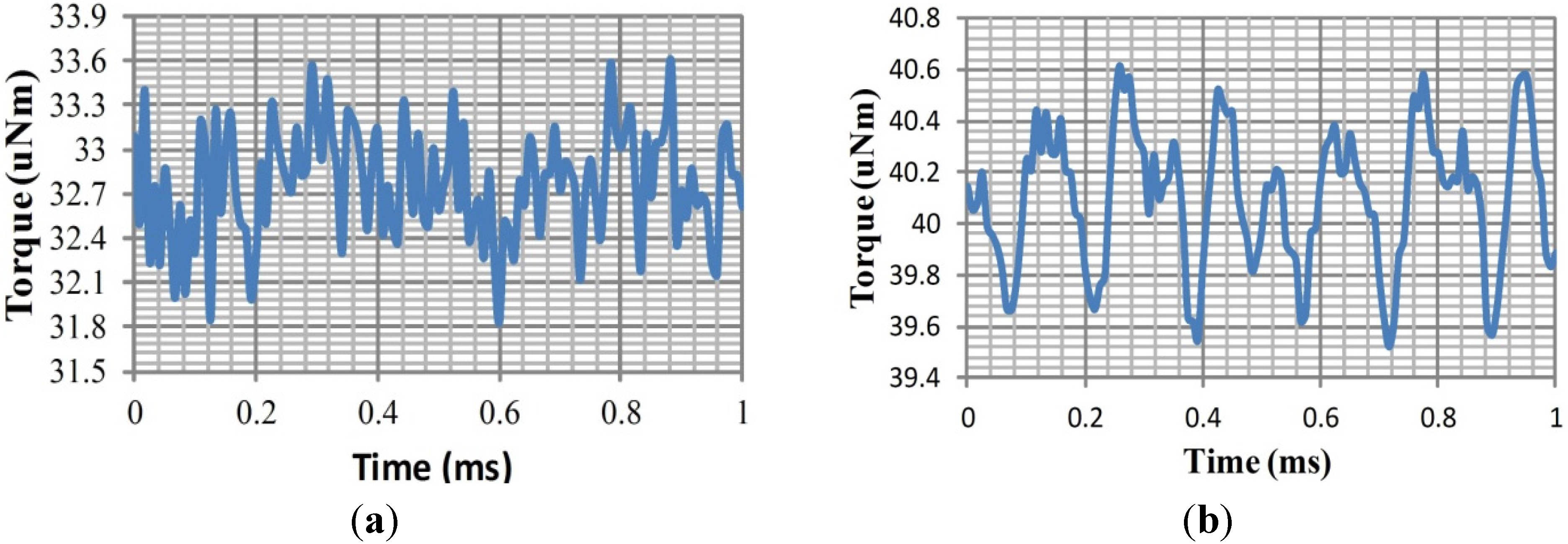
| Torque | 32.1 | 40.97 |
| ( | 87.4 | 93.3 |
| Efficiency | 0.53 | 0.573 |
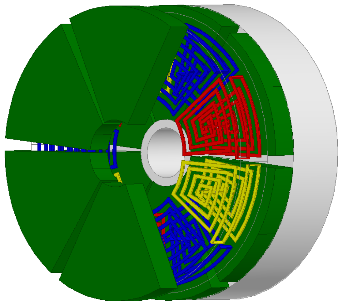
7. 3D FEA Simulation and Experimental Verification
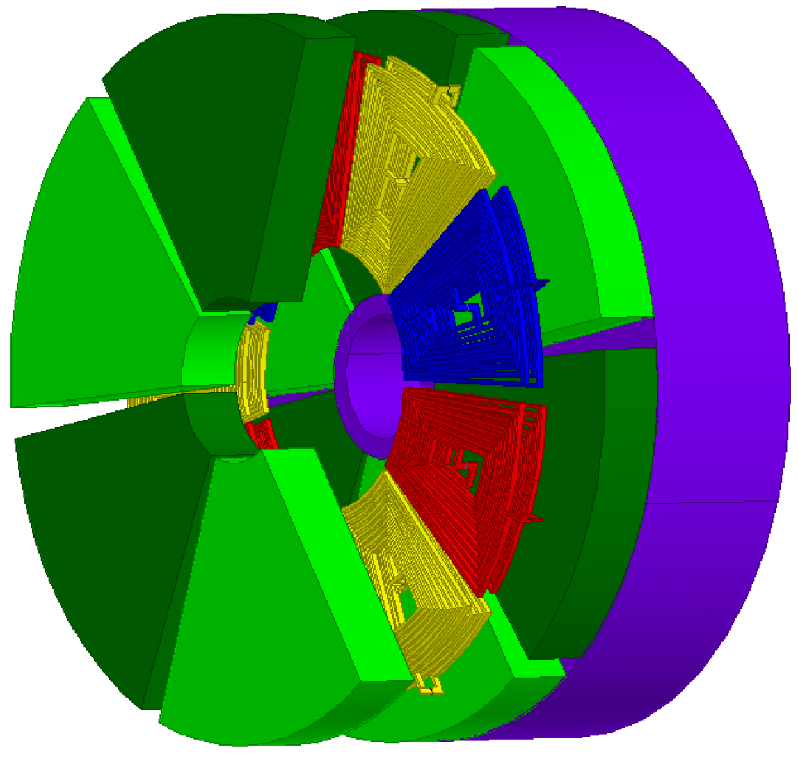
7.1. 3D FEA Simulation Verification


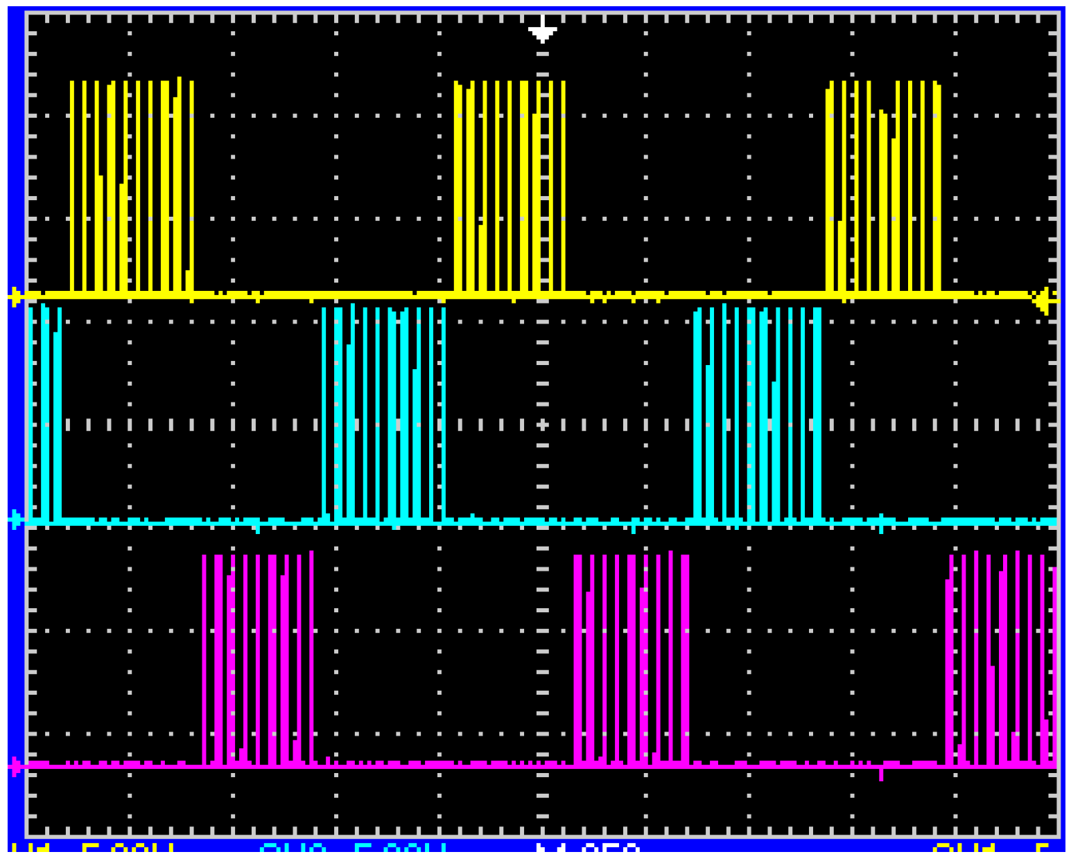
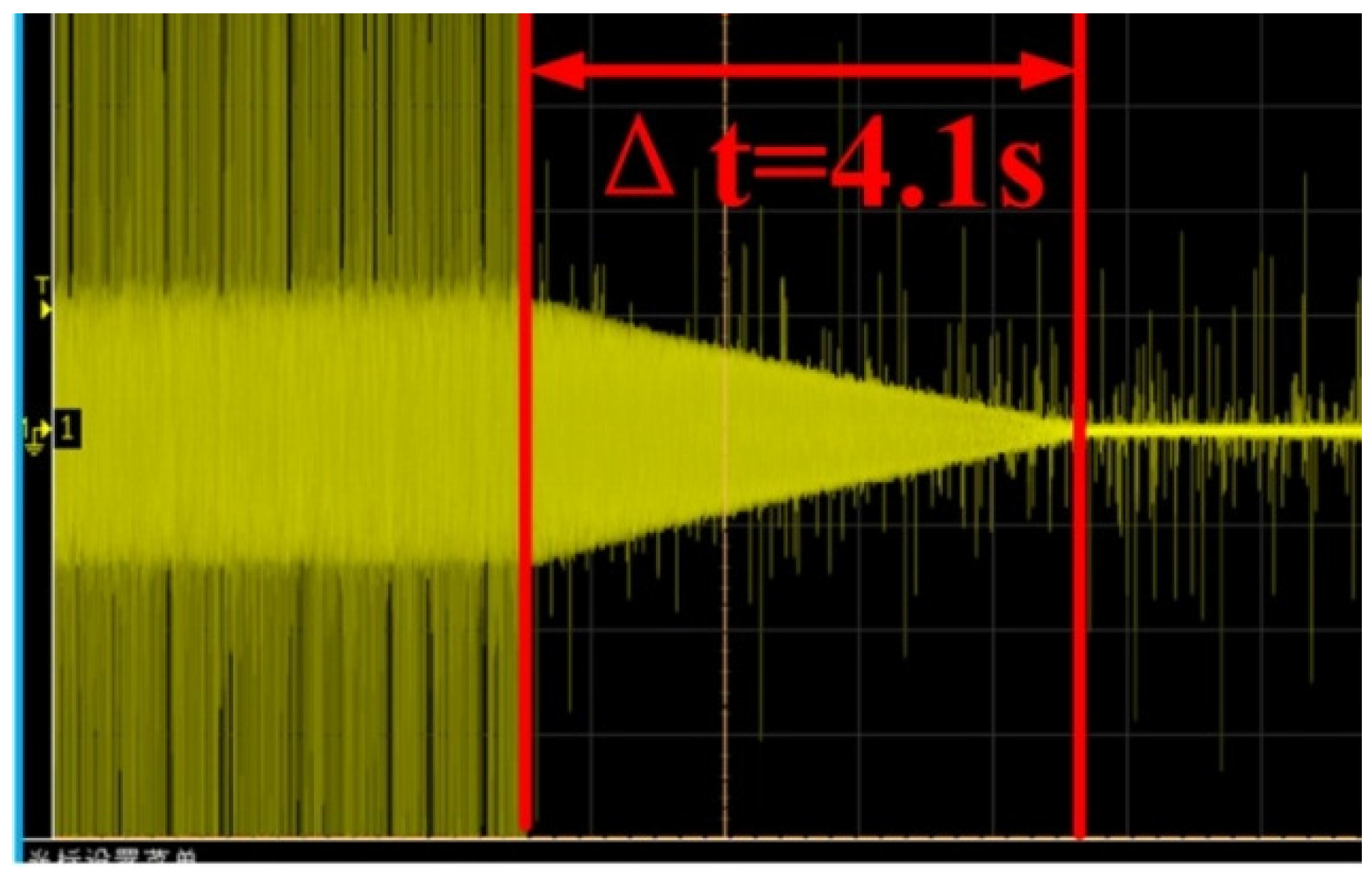
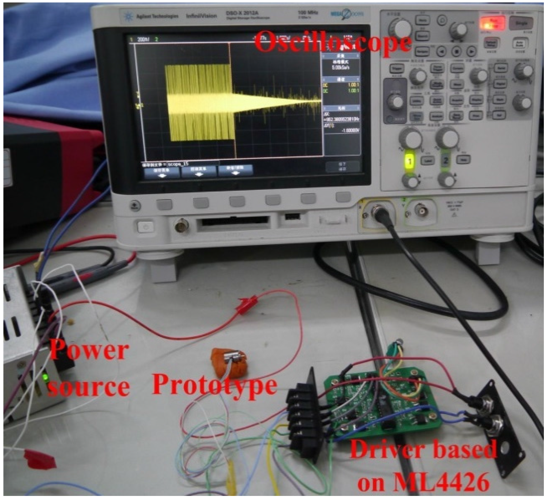
7.2. Experimental Verification


8. Conclusions
Acknowledgments
Author Contributions
Conflicts of Interest
References
- Merzaghi, S.; Koechli, C.; Perriard, Y. Development of a Hybrid MEMS BLDC Micromotor. IEEE Trans. Ind. Appl. 2011, 47, 3–11. [Google Scholar] [CrossRef]
- Achotte, N.; Gilles, P.-A.; Cugat, O.; Delamare, J.; Gaud, P.; Dieppedale, C. Planar brushless magnetic micromotors. J. Microelectromech. Syst. 2006, 15, 1001–1014. [Google Scholar] [CrossRef]
- Ding, X.F.; Mi, C. Modeling of Eddy Current Loss and Temperature of the Magnets in Permanent Magnet Machines. J. Circ. Syst. Comput. 2011, 20, 1287–1301. [Google Scholar] [CrossRef]
- Wagner, B.; Kreutzer, M.; Benecke, W. Permanent magnet micromotors on silicon substrates. J. Microelectromech. Syst. 1993, 2, 23–29. [Google Scholar] [CrossRef]
- Cros, F.; Koser, H.; Allen, M.; Lang, J. Magnetic induction micromachine—Part II: Fabrication and testing. J. Microelectromech. Syst. 2006, 15, 427–439. [Google Scholar] [CrossRef]
- Leifsson, L.; Koziel, S. Multi-fidelity design optimization of transonic airfoils using physics-based surrogate modeling and shape-preserving response prediction. J. Comput. Sci. 2010, 1, 98–106. [Google Scholar] [CrossRef]
- Yang, X.S. Nature-Inspired Metaheuristic Algorithms; Luniver Press: Beckington, UK, 2008. [Google Scholar]
- Talbi, E.G. Metaheuristics: From Design to Implementation; Wiley: New York, NY, USA, 2009. [Google Scholar]
- Yang, X.S. Engineering Optimisation: An Introduction with Metaheuristic Applications; Wiley: New York, NY, USA, 2010. [Google Scholar]
- Yang, X.S. Firefly algorithms for multimodal optimization. Stoch. Algorithms Found. Appl. 2009, 5792, 169–178. [Google Scholar]
- Yang, X.S. Multiobjective firefly algorithm for continuous optimization. Eng. Comput. 2013, 29, 175–184. [Google Scholar] [CrossRef]
- Mahmoudi, A.; Kahourzade, S.; Rahim, N.A.; Hew, W.P. Design, Analysis, and Prototyping of an Axial-Flux Permanent Magnet Motor Based on Genetic Algorithm and Finite-Element Analysis. IEEE Trans. Magn. 2013, 49, 1479–1492. [Google Scholar] [CrossRef]
- Ronghai, Q.; Lipo, T.A. Analysis and modeling of air-gap and zigzag leakage fluxes in a surface-mounted permanent-magnet Machine. IEEE Trans. Ind. Appl. 2004, 40, 121–127. [Google Scholar]
- Huang, Y.; Zhou, T.; Dong, J.; Lin, H.; Yang, H.; Cheng, M. Magnetic Equivalent Circuit Modeling of Yokeless Axial Flux Permanent Magnet Machine with Segmented Armature. IEEE Trans. Magn. 2014, 50, 1–4. [Google Scholar] [CrossRef]
- Huang, Y.; Ge, B.; Dong, J.; Lin, H.; Zhu, J.; Guo, Y. 3-D Analytical Modeling of No-Load Magnetic Field of Ironless Axial Flux Permanent Magnet Machine. IEEE Trans. Magn. 2012, 48, 2929–2932. [Google Scholar] [CrossRef]
© 2015 by the authors; licensee MDPI, Basel, Switzerland. This article is an open access article distributed under the terms and conditions of the Creative Commons Attribution license (http://creativecommons.org/licenses/by/4.0/).
Share and Cite
Ding, X.; Liu, G.; Du, M.; Guo, H.; Qian, H.; Gerada, C. Development of an Axial Flux MEMS BLDC Micromotor with Increased Efficiency and Power Density. Energies 2015, 8, 6608-6626. https://doi.org/10.3390/en8076608
Ding X, Liu G, Du M, Guo H, Qian H, Gerada C. Development of an Axial Flux MEMS BLDC Micromotor with Increased Efficiency and Power Density. Energies. 2015; 8(7):6608-6626. https://doi.org/10.3390/en8076608
Chicago/Turabian StyleDing, Xiaofeng, Guanliang Liu, Min Du, Hong Guo, Hao Qian, and Christopher Gerada. 2015. "Development of an Axial Flux MEMS BLDC Micromotor with Increased Efficiency and Power Density" Energies 8, no. 7: 6608-6626. https://doi.org/10.3390/en8076608
APA StyleDing, X., Liu, G., Du, M., Guo, H., Qian, H., & Gerada, C. (2015). Development of an Axial Flux MEMS BLDC Micromotor with Increased Efficiency and Power Density. Energies, 8(7), 6608-6626. https://doi.org/10.3390/en8076608