Unraveling the Mysteries of Turbulence Transport in a Wind Farm

Abstract

A true physical understanding of the mysteries involved in the recovery process of the wake momentum deficit, downstream of utility-scale wind turbines in the atmosphere, has not been obtained to date. Field data are not acquired at sufficient spatial and temporal resolutions to dissect some of the mysteries of wake turbulence. It is here that the actuator line method has evolved to become the technology standard in the wind energy community. This work presents the actuator line method embedded into an Open source Field Operation and Manipulation (OpenFOAM) large-eddy simulation solver and applies it to two small wind farms, the first one consisting of an array of two National Renewable Energy Laboratory 5 Megawatt (NREL 5-MW) turbines separated by seven rotor diameters in neutral and unstable atmospheric boundary-layer flow and the second one consisting of five NREL 5-MW wind turbines in unstable atmospheric conditions arranged in two staggered arrays of two and three turbines, respectively. Detailed statistics involving power spectral density (PSD) of turbine power along with standard deviations reveal the effects of atmospheric turbulence and its space and time scales. High-resolution surface data extracts provide new insight into the complex recovery process of the wake momentum deficit governed by turbulence transport phenomena.

1. Introduction

Though being one of the fastest growing sources of renewable energy, the wind industry faces a number of challenges today. One of the many difficulties involves an incomplete understanding of the aerodynamics within the wind farm. Wind turbines are progressively more arranged in multiple arrays both onshore and offshore. The associated array performance has a strong correlation to the spatial distance between turbines in an array. This comes at no surprise since a well-designed utility-scale wind turbine can extract up to 50 percent of the wind power passing through its rotor disk area. The resulting viscous shear layer requires some distance to develop and to restore the momentum and energy that have been extracted by an upstream wind turbine. Therefore, in the wind energy community, the accurate computation of the wake momentum deficit downstream of a wind turbine and its recovery governed by wake shear and turbulence transport, see Figure 1, is vital information for wind farm operators in order to maximize energy capture and minimize losses associated with power transfer to the electrical grid. In general, Unsteady Reynolds-Averaged Navier-Stokes (URANS) solvers with the k-ε turbulence model have been used in most cases [1,2,3,4]; however, it has been found that the stability state of the atmosphere can have a profound impact on the array efficiency of a wind farm [5,6,7]. The stability state of the atmosphere is associated with characteristic sheared inflow, surface heating, free-stream turbulence levels, turbulent eddy generation/advection, and the corresponding length and time scales. It is now well accepted that all of the above do affect the recovery of the wake momentum deficit downstream of a wind turbine, which determines the maximum possible power that can be captured by a downstream turbine. It becomes apparent that classical URANS computations are not capable of modeling the underlying wake-turbulence physics. To address this issue, the actuator line method (ALM) has been implemented into a large-eddy simulation (LES) solver developed within the Open source Field Operation and Manipulation (OpenFOAM) framework with the intent to establish a technology capable of modeling wind turbine wakes in a realistic atmospheric boundary-layer (ABL) flow [7,8,9,10,11,12,13,14]. OpenFOAM is a compilation of C++ libraries meant to solve partial differential equations with finite-volume discretization schemes [15].

Figure 1. The Wake of a Wind Turbine (D = Turbine Rotor Diameter).

Figure 1. The Wake of a Wind Turbine (D = Turbine Rotor Diameter).

A typical wind turbine wake can be divided into three main regions, as shown in Figure 1: (i) near wake; (ii) intermediate wake; and (iii) far wake. The near wake is characterized by wake expansion with an associated further decrease in the mean streamwise (axial) velocity and an adverse pressure gradient. This region typically extends between two to three rotor diameters downstream. In the intermediate wake, a mixing (shear) layer develops inside and outside of the model streamtube. This region is also characterized by the tip vortices becoming unstable and merging into larger-scale structures. The end of the intermediate wake is defined as the streamwise distance from the wind turbine at which the mixing layer has reached the rotor centerline. In general, this occurs at a minimum of five to six rotor diameters downstream. In the far-wake region, the bundled tip vortex structures break down into progressively finer scales of inhomogeneous turbulence. After this process is completed, the wake can be considered as fully developed, and the recovery of the wake momentum deficit continues.

Improving array (or wind farm) performance while, at the same time, reducing blade fatigue loads are vital objectives towards reduced Operation and Maintenance (O&M) costs and to an overall reduction in the cost-of-energy (COE) of wind produced power. To date, a detailed understanding of the complex flow physics of wind turbine wakes and their mutual interaction has not been attained that provides the necessary physics-based understanding of the governing turbulence transport phenomena in the wakes of wind turbines. Several researchers have studied different aspects of flow in a wind farm to understand some of these complex flows. Porté-Agel, et al. [16] focused their study on effects of wind direction on turbine wakes and power losses in a large wind farm using LES. They found a strong impact of wind direction on the spatial distribution of turbine-wake characteristics, such as velocity deficit and turbulence intensity. They also studied the effect of wind direction on the distance available for the wakes to recover before encountering other downwind turbines (in full-wake or partial-wake interactions). Another study by Wu and Porté-Agel [17] focused on the atmospheric turbulence effect on wind turbine wakes. They performed a detailed analysis of the turbulent kinetic energy (TKE) budget in the wakes that reveals an important effect of the incoming flow turbulence level on the magnitude and spatial distribution of the shear production and transport terms. Sim et al. [18] studied the space-time resolution of inflow representations for wind turbine loads. They performed the analyses using Fourier-based stochastic simulation of inflow turbulence and investigated loads for a utility-scale turbine in the neutral ABL. Load statistics, spectra, and wavelet analysis representations for different space and time resolutions were studied. VerHulst and Meneveau [19] studied the kinetic energy entrainment in a large wind farm using LES and the lower-order actuator disk method. They found that synthetic vertical forcing at the turbines can have a significant effect on the power extraction and the mean kinetic energy entrainment in a large wind turbine array. Bhaganagar and Debnath [20,21] focused their attention on the near-wake structure and considered the implications of thermal stratification in a stable ABL and the resulting turbulence structures in the near wake. They also studied the effect of mean atmospheric forcing of the stable ABL on the wake. All their studies were performed using the state-of-the-art ALM [13]. On the experimental side, Chamorro and Porté-Agel conducted wind-tunnel experiments on the flow behavior below and above rotor disk height in a wind farm under thermally neutral conditions [22]. Here, the former region has a direct effect on turbine performance, with turbulence statistics reaching equilibrium downstream of the third turbine row (a remaining mystery); the latter region consists of an internal boundary layer, which responds to both the incoming flow and the wind turbines, and an equilibrium layer whose flow conditions are primarily conditioned by the wind farm. A major conclusion concerning the existence of the two outer layers was that large wind farms can be treated as a special case of surface roughness transition. Another experimental work by Chamorro et al. is a milestone in demonstrating the potential performance advantage of staggered wind farms [23]. It was found that momentum recovery and turbulence intensity are affected by the wind farm layout. Further wind-tunnel experiments were performed to quantify the Reynolds number dependence of turbulence statistics in the wake of a model wind turbine [24]. A stronger Reynolds number dependence was observed in the near-wake region but not in the far wake for rotor diameter-based Reynolds numbers larger than approximately 1 × 10⁵.

The present work is purely computational and a stepping stone towards unraveling some of the remaining mysteries governing wind turbine wakes and array performance. A novel idea of splitting axial cross planes “inside” the wind farm, i.e., below maximum turbine tip height, in partitions above and below turbine “hub” height provides some new physical insight into the “mysterious” wake recovery process and power production within an array. This paper focuses on two conceptual case studies, (i) an array of two National Renewable Energy Laboratory 5 Megawatt (NREL 5-MW) wind turbines separated by seven rotor diameters and operating in neutral and moderately-convective (unstable) ABL flow; and (ii) a wind farm consisting of five NREL 5-MW turbines arranged in two staggered arrays of three and two turbines, respectively. The notional NREL 5-MW turbine is chosen in this fundamental study as representative in size and power of next-generation wind deployment. Though no actual data are available for validation, both the atmospheric boundary layer (ABL) solver and actuator line method (ALM) have been validated independently in previous studies [7,13]. The ALM [1,7,8,9,10,11,12,13,14] models the wind turbines as momentum sinks within the OpenFOAM-LES solver. The required high-resolution data extracts for an enhanced physics-based understanding are made possible using a surface-extraction post-processing method, FieldView eXtract DataBase (XDB) workflow. The analysis uses power spectral density (PSD) plots of time-varying power produced by all turbines along with statistics of mean and standard deviation to quantify the effects of the atmospheric stability state and turbine-turbine interaction by means of atmospheric and wake generated turbulence. Reynolds stresses signifying vertical (R₁₃) and lateral momentum transport (R₁₂), as well as Turbulent kinetic energy (TKE) distributions along vertical and horizontal lines are also taken into account for quantifying turbulence transport. Furthermore, the analyses incorporate quantification of fluxes of mass, momentum, power density, and TKE through the axial cross planes.

2. Numerical Methods

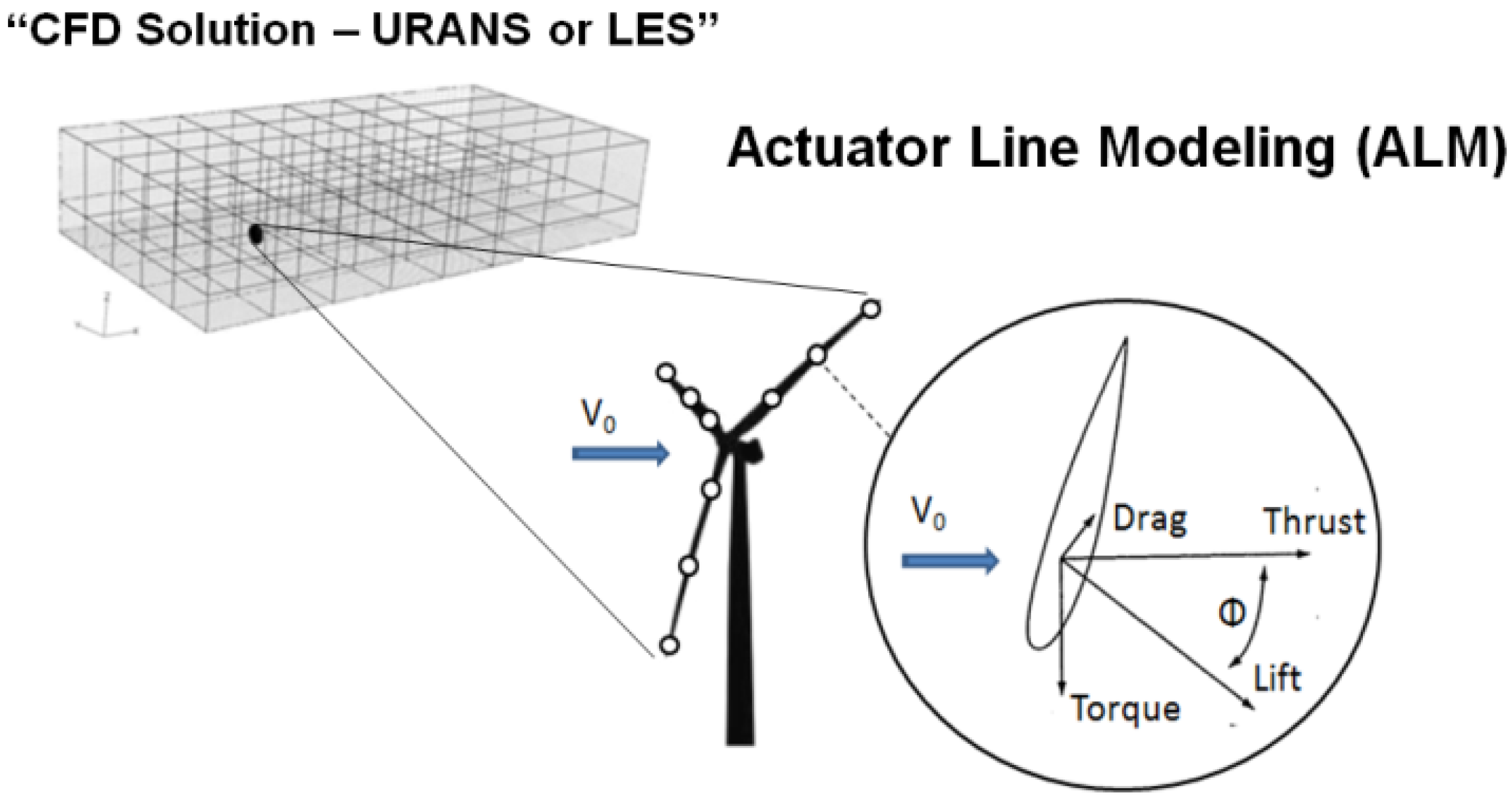
2.1. The Actuator Line Method

The actuator line method (ALM) was originally developed by Sørensen and Shen [1] in an URANS solver to model the wakes of wind turbines, arrays of wind turbines, and wind farms. In the ALM, a blade is discretized as a series of (typically 25–40) actuator points. Sectional lift and drag forces are determined from the local flow velocity and angle of attack (AoA), which are then applied to an airfoil lookup table. Figure 2 shows a schematic of the basic concept of ALM.

Figure 2. Basic concept of the Actuator Line Method (ALM) for modeling wind turbine wakes.

Figure 2. Basic concept of the Actuator Line Method (ALM) for modeling wind turbine wakes.

Each actuator point in Figure 2 has its own aerodynamic force vector, f_N,m = (L_N,m, D_N,m)^T, where L_N,m and D_N,m are lift and drag forces acting on the local actuator element. The indices N and m denote the respective blade and the actuator index along that blade. The lift and drag forces computed at these actuator points are projected onto the background Cartesian grid as body forces to the momentum equation. The force vector, f_N,m, is a point force in space-time that cannot be applied directly as a body-force to the momentum equations of the underlying flow solver, as this would lead to unphysical numerical oscillations. On the contrary, it must be projected onto the grid cells of the surrounding flow field in the form of a body force vector, F_p. The ALM accomplishes this task by using a Gaussian kernel function, η_N,m, as in:

$$F_p(x_p,y_p,z_p,t)=-{\displaystyle \sum _N{\displaystyle \sum _{\text{m}}{f}_{N,m}(x_{N,m},y_{N,m},z_{N,m},t)}{\text{η}}_{\text{N,m}}}$$

(1)

where the subscript p denotes all the grid points that are affected by all actuator elements N, m. The negative sign accounts for the fact that the flow field experiences the equal-and-opposite force that the turbine exerts on the flow field. The Gaussian kernel function, η_N,m, is defined as:

$${\text{η}}_{\text{N,m}}=\frac{1}{{\epsilon }^3{\pi }^{3/2}}\exp \left[-{\left(\frac{\left|r\right|}{\epsilon }\right)}^2\right]$$

(2)

where r is the distance vector between grid point p and actuator element N, m, and ε controls the width of the Gaussian. Equation (2) is such that the volume integral of the projected force vector, F_p, equals the sum of the original actuator segment force or (blade force), f_N,m. It is important to note that the kernel function in Equation (2) is a sole numerical spreading of forces that is required for numerical stability but without any physical reasoning or implications. Recent advances by Jha et al. [12,13,14] suggest that ε should follow an elliptic distribution along the blade span in order to predict accurately spanwise blade loads consistent between various rotor geometries and grid spacing. All the ALM simulations performed in this work use the elliptic distribution of Gaussian spreading width, ε. Sørensen et al. [25] have recently published a comprehensive review work on the study of wind turbine wakes using the ALM.

2.2. The ABLPisoSolver in OpenFOAM (OpenFOAM-LES)

The ABLPisoSolver is an LES solver capable of creating turbulent wind fields under a variety of atmospheric stability conditions. Data from these simulations are used as precursor wind fields to drive an ALM wind farm simulation. The ABLPisoSolver can also be used with uniform inflow conditions, and the generation and advection of turbulent eddies downstream of an ALM modeled wind turbine can be studied. In the ABLPisoSolver, the incompressible Navier-Stokes equations are spatially filtered such that the larger and non-isotropic turbulent scales (large-eddy scales) are directly resolved; the smaller and more isotropic scales are modeled using Smagorinsky model [26] for the sub-grid scale (SGS) viscosity. The filtered continuity equation [11,13] is described as:

$$\frac{\partial {\overline{u}}_j}{\partial x_j}=\text{ 0}$$

(3)

where the overbar indicates the filtering, and ${\overline{u}}_j=u_j-u{\prime }_j$ is the velocity vector of the resolved scale. This velocity vector is the difference of the instantaneous velocity vector, u_j, and the SGS velocity vector, u′_j. The filtered momentum equation reads:

$$\begin{array}{l}\frac{\partial {\overline{u}}_i}{\partial t}+\frac{\partial }{\partial x_j}\left({\overline{u}}_j{\overline{u}}_i\right)\\ =-2{\epsilon }_{ijk}{\text{Ω}}_j{\overline{u}}_k-\frac{\partial \tilde{p}}{\partial x_i}-\frac{\partial }{\partial x_j}\left(R_{ij}^D\right)+\left(\frac{{\rho }_b}{{\rho }_0}-1\right)g_i-\frac{\partial p}{\partial x_i}+{\mathbf{F}}_p\end{array}$$

(4)

Here ε_ijk is the alternating symbol, Ω_j is the rotational rate vector at a location on the planetary surface, $\tilde{p}$ is the deviation of the resolved pressure, $\overline{p}$, from the hydrostatic pressure plus the SGS energy contribution (all normalized by the density, ρ₀), ${R_{ij}}^D$ is the deviatoric part of the SGS stress tensor, the buoyancy term containing the density ratio ρ_b/ρ₀ is handled by the Boussinesq approximation, g_i is gravity, and $\partial p/\partial x_i$ is a constant horizontal-mean driving pressure gradient. Viscous terms are not included in Equation (4) due to the assumption of high Reynolds number flow.

The grid force vector (or body force), F_p, describes the momentum forcing due to ALM governed by Equation (1). A finite-volume method on unstructured meshes is used to solve the governing equations with all variables being cell-centered and collocated on the grid. Fluxes of velocity at the finite-volume faces are interpolated similar to the work of Rhie and Chow [27] in order to avoid pressure-velocity decoupling. Further interpolation from cell centers to faces is handled with a blend of linear (second-order central differencing) and midpoint (second-order differencing with equal weighting regardless of mesh stretching) with a small amount of first-order upwinding. The classical PISO (Pressure-Implicit Splitting Operation) algorithm by Issa [28] is used for time advancement, which is an implicit predictor/corrector scheme. The implicit terms are integrated in time using second-order Crank-Nicolson discretization. We use one predictor followed by three corrector steps. The time steps used in the simulations are determined by a more stringent condition than the standard CFL criterion. For all cases considered in this work, the time step is chosen such that the blade tip does not traverse more than one grid cell per time step in the innermost refinement zone. The Poisson equation for the pressure is solved using a geometric agglomerated algebraic multigrid (GAMG) solver. The message-passing interface (MPI) is used for solver parallelization.

2.3. Computational Grids and Simulation Methodology

A typical baseline grid for an ALM OpenFOAM-LES simulation contains several refinement zones. Figure 3 indicates the end of the outer refinement zone (red rectangle) and the beginning of the innermost refinement zone (green rectangle). In general, the outer grid dimensions span from −5D to +10D in the streamwise and −5D to +5D in the other two directions with the location of the first rotor being the reference point. The grid spacing in the outer refinement zone is approximately 10 m. These grid dimensions are based on common practice used in the wind energy community [7,8,9,10,11,12,13,14]. The innermost refinement region starts 2.5D upstream of the first turbine row and extends all the way into the wake. For the best LES accuracy, the grid spacing in the innermost refinement zone is uniform with a cell aspect ratio of approximately one. In case of the NREL 5-MW turbine, it was found that 25 grid points are needed along the actuator line to compute integrated rotor thrust and torque to within 2% of a reference case with grid refinement. This results in a near-turbine grid spacing of approximately 2.5 m. In other words, this results in turbulent eddies being directly resolved down to length scales close to the blade tip chord. A baseline grid used for ALM turbine-turbine interaction simulations, as shown in Figure 3a, contains a total of approximately 15–20 million cells with the turbines being spaced 7 rotor diameters apart from each other. The conceptual arrangement with 5 wind turbines considered in this work, as shown in Figure 3b, contains a total of 32 million cells. Here the turbines in each of the two arrays are spaced 6 rotor diameters apart, and the spanwise distance between the arrays is 2.5 rotor diameters. For a typical tip speed ratio of about 5 for utility-scale wind turbine rotors at an average wind speed, e.g., V_Wind = 8 m/s, this means that it takes approximately 40 rotor revolutions (or 250 s of real time) for the wake to exit the computational domain. On 512 2.6 GHz processors, such a baseline run of the turbine-turbine interaction problem using the ALM OpenFOAM-LES solver requires about 5 days of wall-clock time, and the 5-turbine case requires about 10 days of wall-clock time to simulate 500 s of real time.

Figure 3. Nested grids used for the ABL-ALM simulations. (a) Turbine-Turbine Interaction; (b) 5-Turbine Wind Farm.

Figure 3. Nested grids used for the ABL-ALM simulations. (a) Turbine-Turbine Interaction; (b) 5-Turbine Wind Farm.

2.4. FieldView XDB Workflow

Post-Processing of CFD data is often regarded as mundane and straight forward; however, without careful thought about the post-processing workflow required for data analysis, an investigator would not be able find the scientifically valuable gems contained within a dataset, particularly for a large unsteady dataset. For example, the flux analyses performed in this work and further described in Section 3.3.2. and Section 3.3.3. required 10 rotor revolutions of data and would have required up to 10 Terabytes of volume grid and solution data files written and saved for processing, exceeding the user storage policy of the Penn state compute cluster. In this work, the CFD post-processing tool FieldView [29] was used to reduce the data by creating iso-surface and coordinate-surface extracts that were then used for flow-field visualizations, see also Bashioum et al. [30], and to integrate turbulent kinetic energy and momentum flux for detailed wake analyses.

To create these surfaces, a concurrent set of batch jobs were executed across up to six compute nodes, each in shared-memory parallel mode using up to 16 cores and 32 GB of memory. Each batch job read the OpenFOAM volume data files and created iso-surfaces of vorticity magnitude, coordinate and arbitrary planar surfaces. Once these surfaces were saved to the disk, the volume data were deleted. Each surface extract has the same grid resolution as the original volume grid; however, all the FieldView XDB files are 30 times smaller than the original OpenFOAM volume data. The XDB file contains the iso-surface geometry along with the corresponding scalar quantities of velocity and vorticity magnitudes. For the coordinate and planar iso-surfaces, the time-variant mean and instantaneous velocity vector, vorticity vectors, and turbulent kinetic energy were saved. The XDB files were then transferred to a local workstation where the visualizations were created and further data analyses (such as momentum integrations) were performed.

Because the user no longer has to load very large unsteady datasets, the workflow outlined above enabled the correlation of flow-field visualizations against detailed wake-integration analyses. The OpenFOAM solver creates a flood of CFD data, on the order of 10 Terabytes of volume data that would have been extremely tedious, if not impossible, to post-process using contemporary volume data and file-based serial post-processing. Once these surfaces were written to disk, further post-processing was tractable as demonstrated by the results presented in Section 3.3.3.

3. Results and Discussion

In the following, two conceptual case studies of the ALM OpenFOAM-LES solver are presented. The first example concerns an array of two NREL-5MW turbines, a layout of which is shown in Figure 3a. The effect of the atmospheric stability state on turbine-turbine interaction is quantified using mean and standard deviation of turbine power, wake-velocity profiles, Reynolds stresses, and the associated turbulent kinetic energy (TKE) downstream of the turbines. For the second example, a small wind farm consisting of five turbines arranged in two adjacent staggered arrays, a layout of which is shown in Figure 3b, is considered under moderately-convective atmospheric conditions. In addition to mean power and standard deviation, a number of integration planes are defined with the intent to investigate the net streamwise turbulent momentum transport through the rotor disk area. Results obtained are discussed with an emphasis towards an enhanced physics-based understanding of the evolution of turbine power within an array.

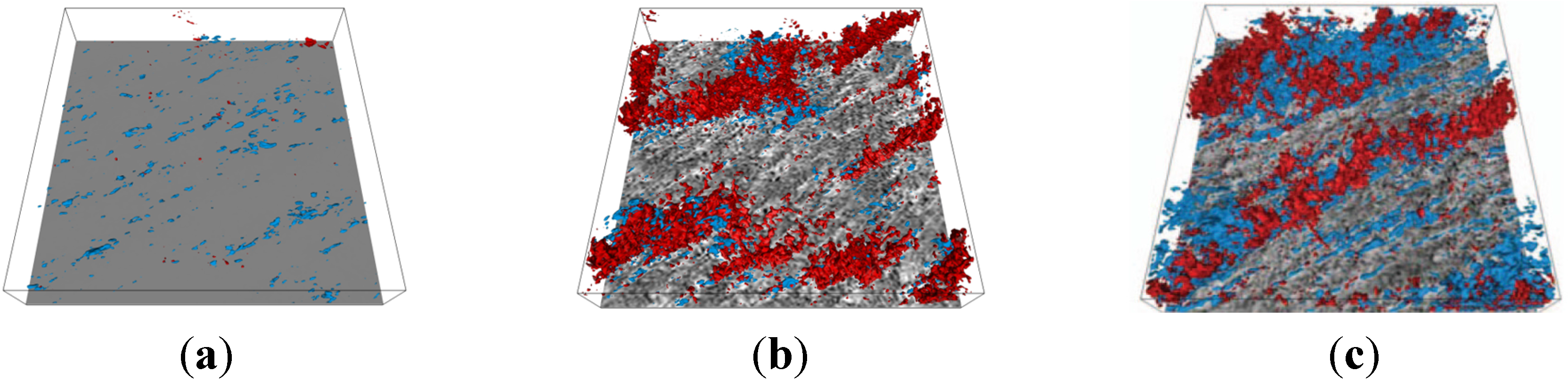
3.1. Atmospheric Boundary Layer Precursor Simulations (OpenFOAM-LES)

For the turbine-turbine interaction problem, two stability states were considered, i.e., a neutral boundary layer (NBL) and a moderately-convective boundary layer (MCBL) with a surface-temperature flux, q_s, of 0.04 km/s, both with a surface roughness, z₀, of 0.001 m typical of a marine ABL over calm sea. The wind farm consisting of five wind turbines was considered under MCBL conditions only, with the MCBL precursor produced with a surface roughness of z₀ = 0.2 m typical of a flat onshore terrain [31]. For all ABL precursor simulations, a horizontally-averaged mean wind speed of 8 m/s is obtained at hub height (90 m) all through the domain by adjusting the streamwise pressure gradient. A constant grid spacing of 10 m was used through the 3 km × 3 km × 1 km domain. Both ABL precursor simulations were performed until a quasi-stationary state was achieved, i.e., after 18,000 s for the NBL case and 12,000 s for the MCBL case. The quasi-stationary state is determined by the convergence of friction velocity, u*. After achieving the quasi-stationary state, data to be used in the ALM simulations were stored for subsequent 2000 s at an interval of 0.5 s. These precursor data serve as boundary condition at the inlet planes for the ALM simulations. Turbulence statistics applied to the ABL precursor simulations are reported in previous papers [12,13,14]. Table 1 summarizes the primary integral boundary-layer parameters, which were obtained by averaging over the last 4000 s of the respective precursor simulations.

Table 1. Integral boundary-layer parameters of precursor simulations, OpenFOAM-LES. (Surface heat flux q_s = 0.04 km/s for MCBL cases).

Precursor Simulation	Stability	Ug (m/s)	Ih (%)	u* (m/s)	w* (m/s)	zi (m)	−zi/L	t* (min)
Turbine-Turbine Interaction (z0 = 0.001 m)	NBL	9.1	4.9	0.27	0	755	0	46
	MCBL	8.0	7.0	0.33	0.99	745	10.99	12
5-Turbine Wind Farm (z0 = 0.2 m)	MCBL	10.4	8.9	0.53	1.00	765	2.70	13

Table 1. Integral boundary-layer parameters of precursor simulations, OpenFOAM-LES. (Surface heat flux q_s = 0.04 km/s for MCBL cases).

Precursor Simulation	Stability	Ug (m/s)	Ih (%)	u* (m/s)	w* (m/s)	zi (m)	−zi/L	t* (min)
Turbine-Turbine Interaction (z0 = 0.001 m)	NBL	9.1	4.9	0.27	0	755	0	46
	MCBL	8.0	7.0	0.33	0.99	745	10.99	12
5-Turbine Wind Farm (z0 = 0.2 m)	MCBL	10.4	8.9	0.53	1.00	765	2.70	13

In Table 1, U_g is the geostrophic wind as a result of a horizontally-averaged mean wind speed at hub height of 8 m/s. The turbulence intensity at hub height, I_h, is defined as I_h = [1/3(<u’u’>²+<v’v’>²+<w’w’>²)]^1/2/<U>_h. Table 1 also contains the convective velocity, w* = (g·q_s·z_i/Θ₀)^1/3 where Θ₀ is the potential temperature and z_i is the boundary-layer height determined by the height at which the time- and horizontally-averaged total vertical temperature flux has a minimum. The ratio of the boundary-layer height to the Obukhov length is –z_i/L with the Obukhov length defined as L = −(Θ₀·u*³)/(g·q_s·κ) where κ = 0.4 is the von Kármán constant. The large-eddy turnover time, t*, is defined as t* = z_i/u* in the NBL case and as t* = z_i/w* in the MCBL cases. It can be seen that the boundary-layer height, z_i, is similar for all cases; however, the stability state as characterized by −z_i/L is particularly reflected in I_h, u*, and w*, with the case of highest surface roughness, z₀, showing the highest friction velocity, u*. Of particular note is the difference in the large-eddy turnover time, t*, between the NBL and MCBL cases as will be further discussed in Section 3.2 with respect to the wake recovery process.

Figure 4 comprises some turbulence visualizations of the three precursor simulations; the blue iso-surfaces define low-speed streamwise velocity fluctuations at −1.25 m/s, the red iso-surfaces show vertical updrafts at +1.00 m/s. It can be seen that practically no vertical updrafts are present in the NBL case, while the unstable (MCBL) cases reveal organized vertical structures.

Figure 4. Iso-surfaces of instantaneous streamwise (blue, −1.25 m/s) and vertical (red, +1.00 m/s) velocity fluctuations in atmospheric boundary-layer precursor simulations (OpenFOAM-LES). (a) NBL (z₀ = 0.001 m); (b) MCBL (z₀ = 0.001 m); (c) MCBL (z₀ = 0.2 m).

Figure 4. Iso-surfaces of instantaneous streamwise (blue, −1.25 m/s) and vertical (red, +1.00 m/s) velocity fluctuations in atmospheric boundary-layer precursor simulations (OpenFOAM-LES). (a) NBL (z₀ = 0.001 m); (b) MCBL (z₀ = 0.001 m); (c) MCBL (z₀ = 0.2 m).

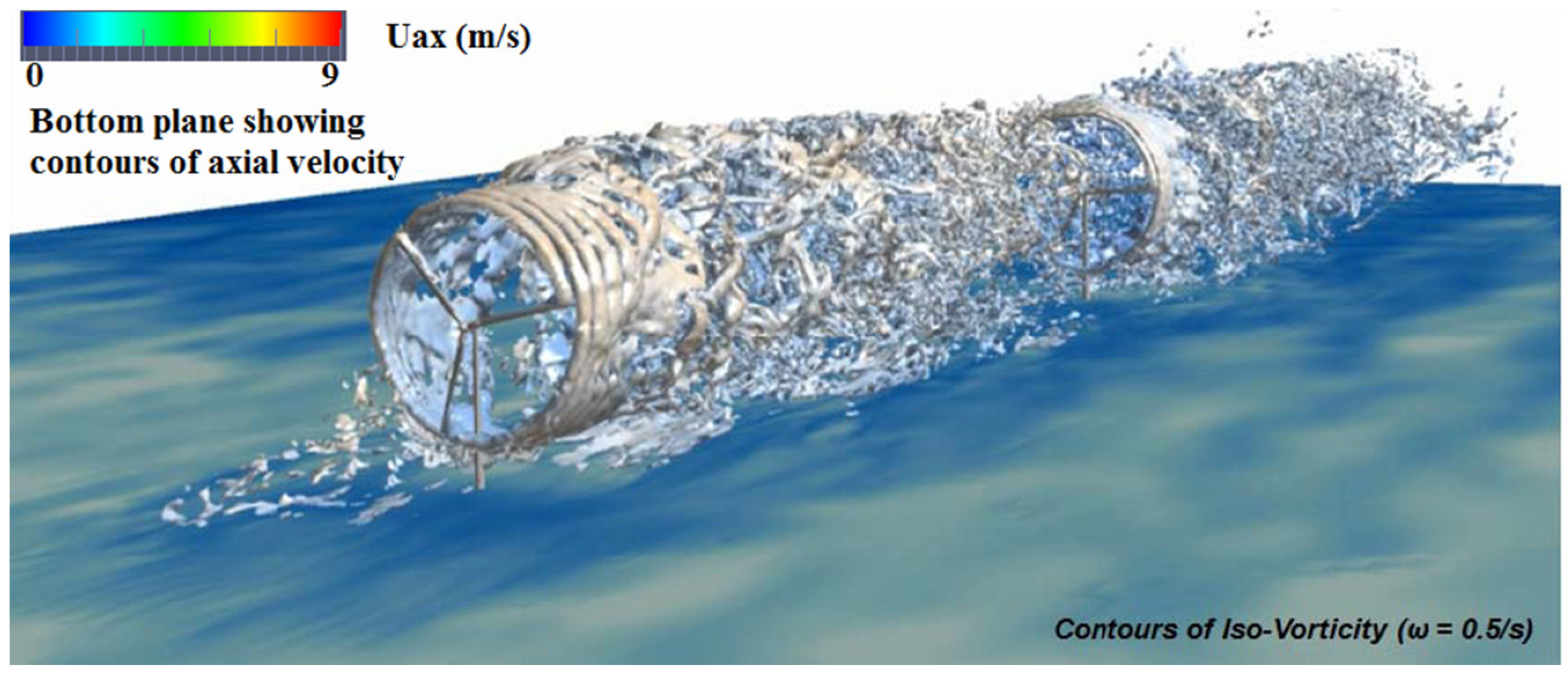
3.2. A Turbine-Turbine Interaction Problem (ALM OpenFOAM-LES)

An array of two NREL-5MW wind turbines was modeled using the ALM OpenFOAM-LES solver. The NREL-5MW wind turbine is a notional large wind turbine of 126 m diameter intended for offshore operation. It was developed by the National Renewable Energy Laboratory (NREL) and is the reference turbine for various trade studies for the deployment of offshore wind energy in the U.S. [32]. Figure 5 illustrates iso-surface of vorticity magnitude 0.5 1/s extracted from the computed flow field via the XDB methodology described earlier. The second turbine (Turbine 2) is located 7 diameters downstream of the first turbine (Turbine 1). The ALM domain of 3 km × 3 km × 1 km is forced by equilibrium ABL turbulence under neutral and unstable conditions as described above. It is seen in Figure 5 that the tip vortices trailing downstream of the first turbine remain stable for approximately four revolutions. It is also apparent that the flow becomes dominated by turbulent eddy motion before interacting with the second (downstream) turbine and even more so downstream of the second turbine. Figure 5 also indicates that tip vortices break down sooner downstream of Turbine 2 than they do downstream of Turbine 1. It is shown later in this paper that the enhanced turbulence in the inflow plane to Turbine 2 results in a higher standard deviation of turbine power.

Figure 5. Turbine-Turbine interaction in NBL flow (NREL 5-MW Turbines, V_Wind = 8 m/s).

Figure 5. Turbine-Turbine interaction in NBL flow (NREL 5-MW Turbines, V_Wind = 8 m/s).

Figure 6 shows an axial plane through the rotor hub colored with instantaneous contours of velocity magnitude for NBL flow at time t = 2000 s of the ALM simulation. A CAD model of the NREL 5-MW turbine has been added to the figure to illustrate the position of the actuator lines (or rotor blades) at this particular instant in time. It can be seen that the upper (above turbine hub height) sheet of tip vortices becomes unstable and eventually large structures break down in the wake into progressively finer structures of turbulence. It is interesting to note that the lower (below turbine hub height) sheet of tip vortices becomes unstable much sooner than its upper counterpart. This is attributed to higher shear in the lower parts of the atmospheric surface layer. This is expected to affect the wake profile for the upper and lower halves of the rotor disk and hence the wake recovery pattern. In addition, Figure 6 shows that the root vortices appear less strong, which is attributed to the transition region from the root airfoil section into a cylindrical section close to the hub that essentially does not produce any aerodynamic lift. The actual root vortices are hence spread over that transition region and thus appear to be weaker than the tip vortices.

Figure 6. Instantaneous contours of velocity magnitude (NREL 5-MW Turbine 1, V_Wind = 8 m/s).

Figure 6. Instantaneous contours of velocity magnitude (NREL 5-MW Turbine 1, V_Wind = 8 m/s).

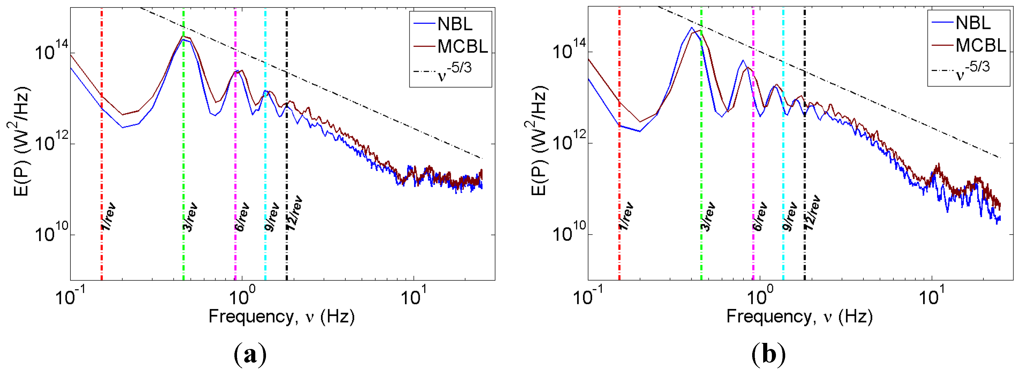
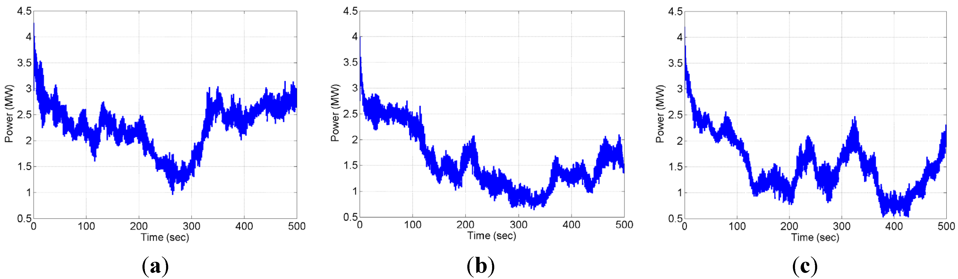
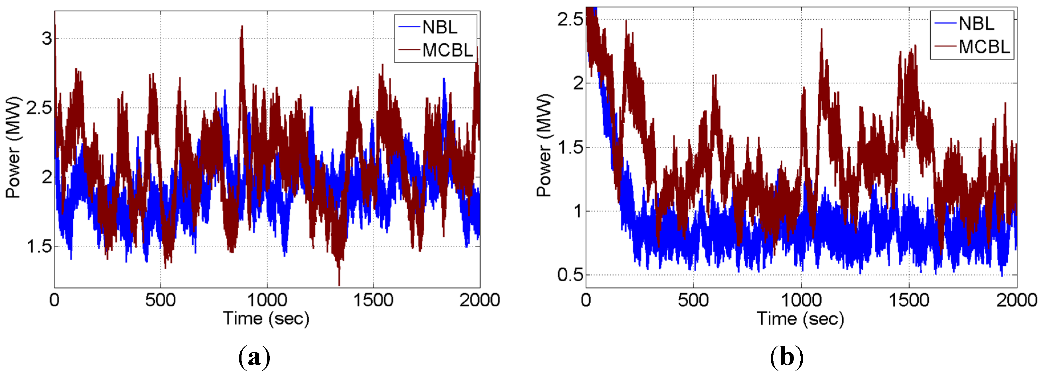
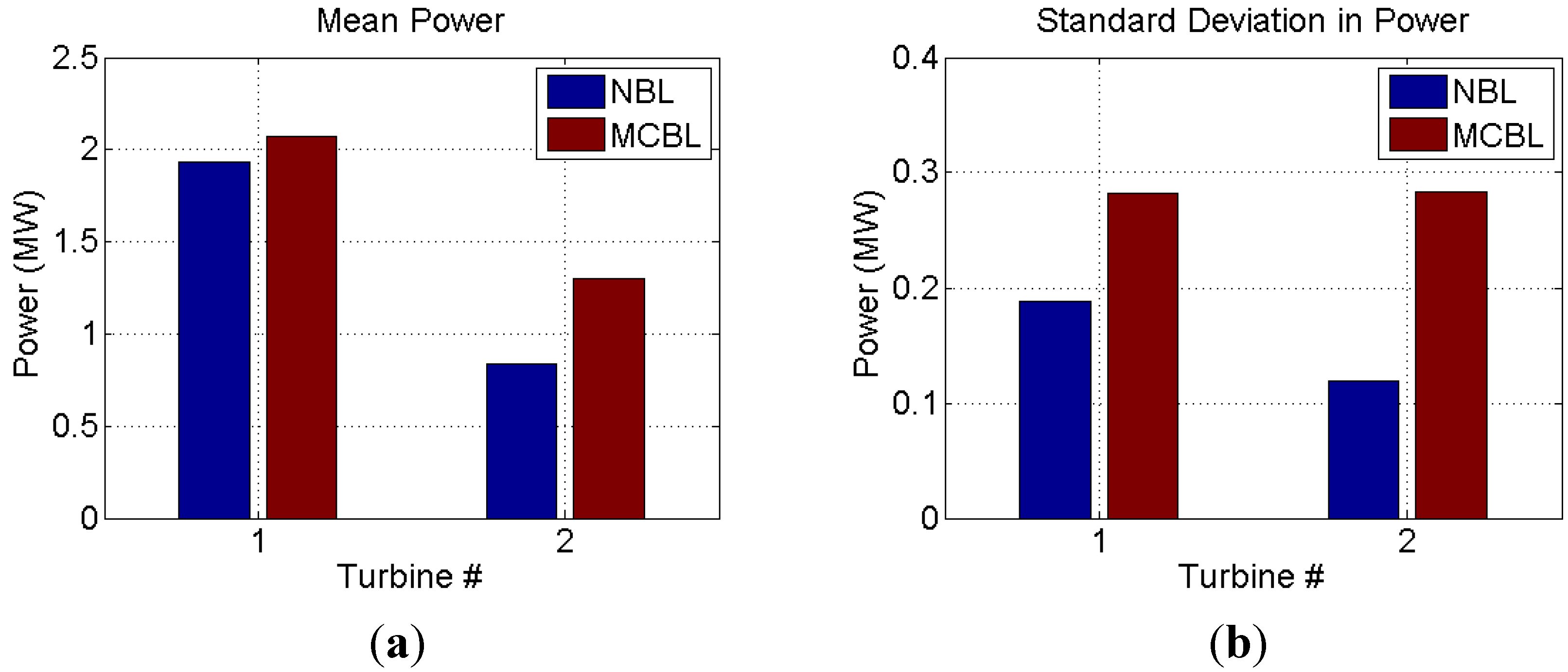
3.2.1. Turbine Power

Figure 7 illustrates time series over a total of 2000 s (approx. 300 rotor revolutions) of turbine power for both turbines and for both stability states, NBL and MCBL. Several qualitative observations can be made. In the NBL case, turbine power drops significantly from Turbine 1 to Turbine 2. This, as will be supported later by Reynolds stresses, is due to a slow recovery process of the wake momentum deficit in the wake of Turbine 1 in NBL conditions where turbulent mixing processes are relatively weak. Furthermore, Figure 7a illustrates that, in NBL flow (blue line), the power produced by Turbine 1 responds to atmospheric eddy-time scales. For example, one can notice responses of the order of 100 s to about 600 s. As far as Turbine 2 under NBL conditions in Figure 7b is concerned, it is apparent that a significant power loss occurs after approximately 200 s when the wake of Turbine 1 starts interacting with Turbine 2. This time delay in turbine response is consistent with a mean wind speed of 8 m/s at hub height and a reduction of this axial velocity, i.e., axial induction due to power extraction by Turbine 1. The situation changes in MCBL flow (brown line). As for Turbine 1, Figure 7a shows a time series of turbine power that appears to have a similar mean compared to the NBL case but exhibits much stronger variations in the turbine response and also at different time scales. These larger variations are attributed to vertical updrafts, see Table 1 and Figure 4b, as a result of the surface temperature flux in the case of MCBL flow. Interestingly, the power of Turbine 2 in Figure 7b is overall higher in the MCBL case than in the NBL. It will be confirmed with Reynolds stresses in Section 3.2.2. that this is due to enhanced turbulent momentum transport down to the surface, thus leading to accelerated recovery of the wake momentum deficit in the wake of Turbine 1 for MCBL compared to NBL flow. Further comparison of NBL and MCBL cases in Figure 7b reveals that the MCBL case shows much higher variations about the mean when compared to the NBL case. This is again attributed to the presence of strong updrafts in the MCBL flow.

Figure 7. Time series of power (Turbine-Turbine Interaction Problem, V_Wind = 8 m/s). (a) Turbine 1; (b) Turbine 2.

Figure 7. Time series of power (Turbine-Turbine Interaction Problem, V_Wind = 8 m/s). (a) Turbine 1; (b) Turbine 2.

A detailed look at the power spectral density (PSD) of turbine power is useful to gain insight into the frequency content in the time histories shown in Figure 7. Note that, for perfectly isotropic and homogeneous turbulence, the slope would be expected to be −5/3 according to Kolmogorov’s law. Figure 8 shows plots of PSD of turbine power for both stability states; the −5/3 slope is shown for reference. Data were obtained from a statistical analysis of 1700 s of 2000 s of the time series in Figure 7. The first 300 s were not considered to let the wake from Turbine 1 go well past Turbine 2. The sampling frequency was 50 Hz corresponding to the simulation time step of 0.02 s, thus resulting in 85,000 samples. In order to get smooth spectra, 85 windows of 1000 samples each were used, and the mean of the PSD of each of these windows was computed and presented in Figure 8. For both turbines and both stability states, the dominant frequency is the blade passage frequency 3/rev, i.e., about 0.45 Hz (for a mean rotational speed of 9.16 RPM). The higher harmonics of n* (3/rev) are also visible in Figure 8. They occur because of the fluctuating velocity components that result in a different incoming mean shear flow for every single blade revolution. It can also be observed that the peak frequencies of Turbine 2 are not perfectly aligned with the multiples of rotational frequency. This is attributed to the variable rotor speed of Turbine 2 in response to the turbulent wake from Turbine 1 since the downstream turbine seeks the design tip speed ratio (TSR). For both turbines in Figure 8, the NBL and MCBL stability states mainly differ in PSD for frequencies lower than 0.45 Hz (3/rev) and higher than 1.8 Hz (12/rev), with the latter stability state having higher energy content than the former. Interestingly, there are similar PSD values of the exact multiples 3/rev up to 12/rev.

Figure 8. Power spectral density of power (Turbine-Turbine Interaction Problem, V_Wind = 8 m/s). (a) Turbine 1; (b) Turbine 2.

Figure 8. Power spectral density of power (Turbine-Turbine Interaction Problem, V_Wind = 8 m/s). (a) Turbine 1; (b) Turbine 2.

Figure 9 shows the mean and standard deviation of turbine power, computed over the 1700 s of the time-series data of turbine power in Figure 7, for both turbines and both stability states. While Turbine 1 does not show a large effect of the atmospheric stability state on turbine power, Turbine 2 shows an increase in power by 40% in MCBL as opposed to NBL conditions. As is shown later, this is due to an accelerated wake recovery process in the presence of strong updrafts under MCBL conditions that enhance turbulent mixing and momentum transport in the wake of Turbine 1. Figure 9b reveals that the standard deviation in turbine power shows a significant increase under MCBL conditions when compared to NBL flow. This is once more attributed to higher turbulence content in the MCBL compared to the NBL. The spectra in Figure 8 are only weakly indicative of this; however the time series in Figure 7 clearly show the larger variations about the mean turbine power in MCBL flow that are integrated to the standard deviations shown in Figure 9b. It is worth mentioning that, while the MCBL appears to be advantageous with respect to array efficiency, the significant increase in standard deviation also leads to an increase in blade fatigue [33,34,35].

Figure 9. Mean and standard deviation of power (Turbine-Turbine Interaction Problem, V_Wind = 8 m/s). (a) Mean; (b) Std. Deviation.

Figure 9. Mean and standard deviation of power (Turbine-Turbine Interaction Problem, V_Wind = 8 m/s). (a) Mean; (b) Std. Deviation.

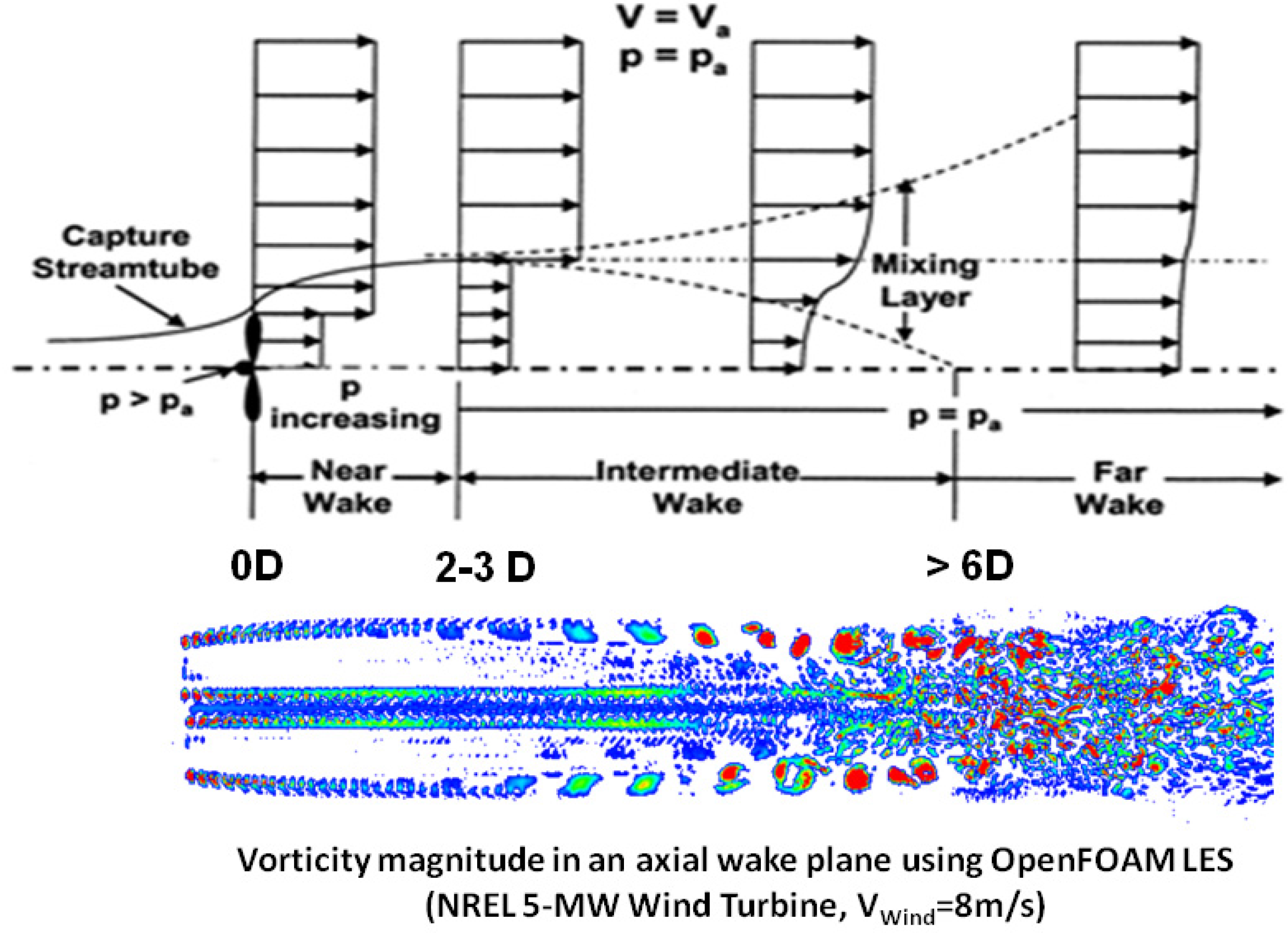
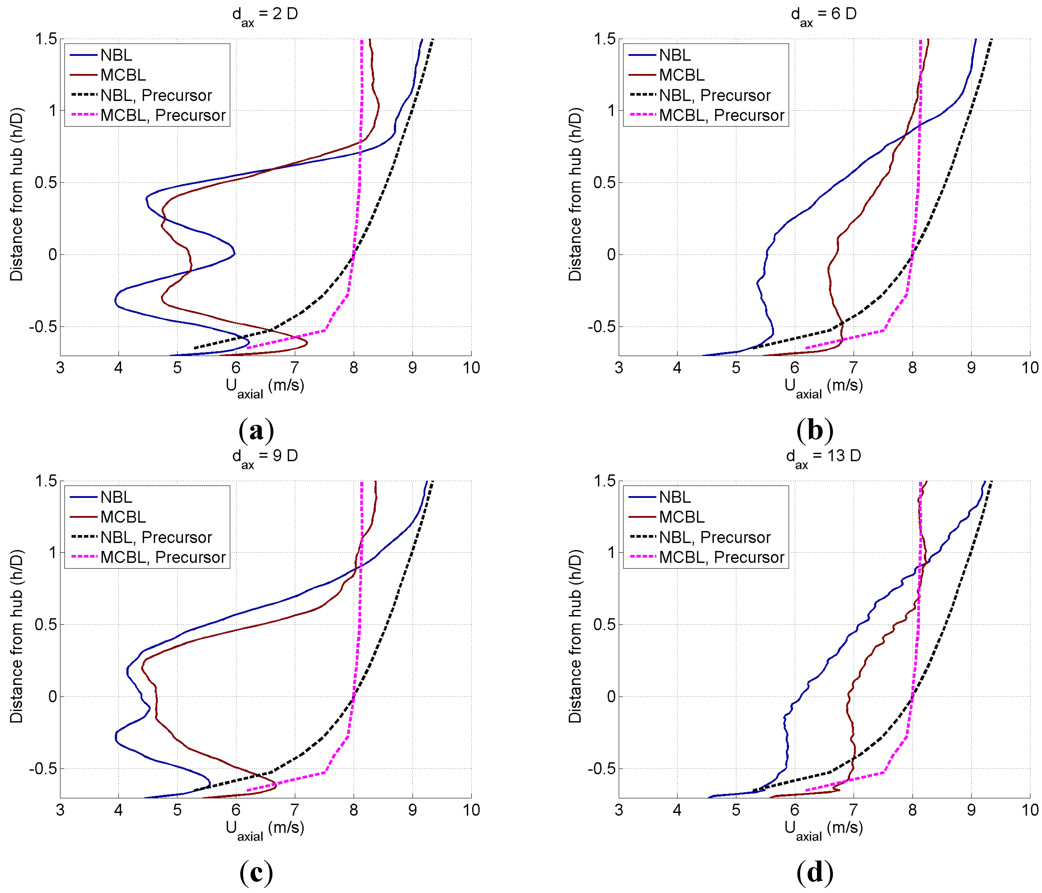
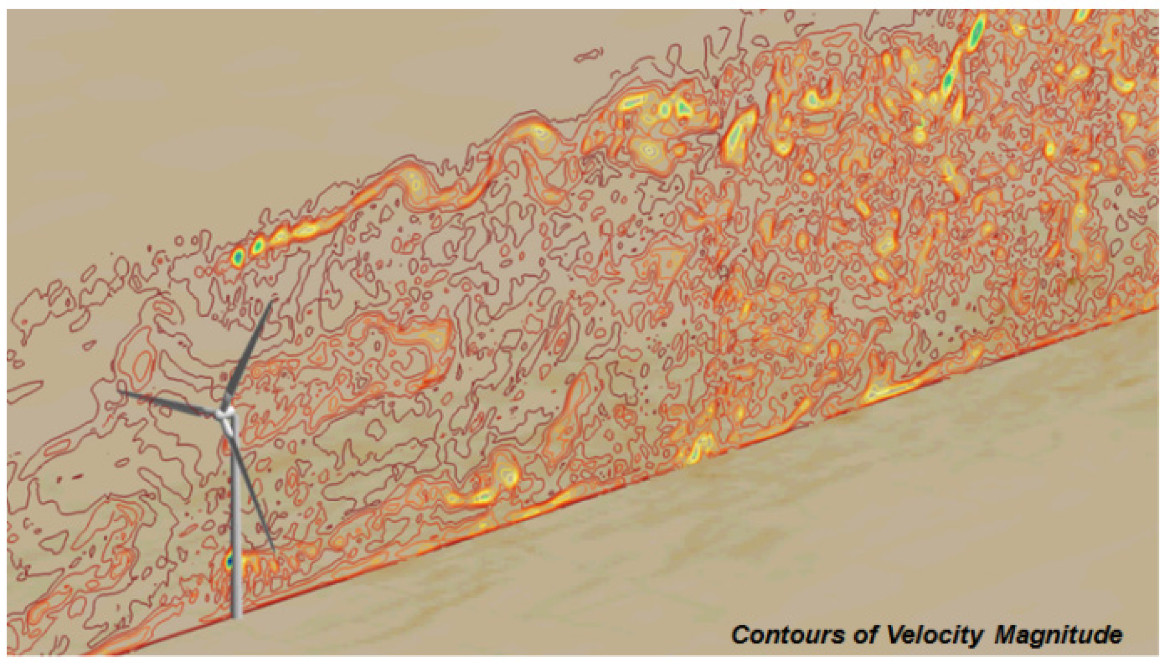
3.2.2. Wake Velocity Deficit

It was noted in the previous section on turbine power that the time series, spectra, and statistics of turbine power for the two stability states are different. These differences are more pronounced for Turbine 2. This was attributed to the difference in turbulent mixing pattern and wake recovery process for the two stability states. This is further supported by analyzing the wake profiles. Figure 10 shows velocity distributions in the wake of both wind turbines and at both stability states, i.e., NBL and MCBL flow. The mean velocity profiles obtained from the precursor simulations of the NBL and MCBL are shown for comparison. It can be seen that both mean ABL precursor velocity profiles do have the same axial velocity of 8 m/s at hub height. Due to its higher turbulence content the MCBL velocity profile has less shear, though higher skin friction, compared to the NBL. This is consistent with the behavior of turbulent boundary layers. Figure 10a shows mean velocity profiles at a distance of two rotor diameters downstream of Turbine 1. In comparison to the corresponding precursor ABL velocity profile, it is evident that momentum extraction is lowest at the hub and highest close to the blade tips, which is consistent with wind turbines producing the maximum torque per unit length close to the 80% spanwise station along the blade and in the upper half of the rotor disk. An interesting observation is that the momentum/power extraction at Turbine 1 appears to be more uniform in MCBL compared to NBL conditions. This is likely due to the fact that the mean MCBL velocity profile has less shear compared to the NBL velocity profile. Furthermore, under NBL conditions (blue line), the wake has recovered noticeably less below hub height than for the MCBL case, even though the mean streamwise wind speed below hub height is less than in the MCBL case. At a distance of six rotor diameters downstream of Turbine 1 in Figure 10b, both wake velocity profiles exhibit similar trends; however, it is evident that the MCBL wake velocity deficit has recovered substantially more than in NBL flow. This is consistent with the power of Turbine 2 being higher in MCBL compared to NBL flow. Note that Figure 10b essentially shows the inflow one rotor diameter upstream of Turbine 2 (or six diameters downstream of Turbine 1). It is apparent from Figure 10b that the mean shear is not the primary driver for the momentum recovery in the wake but that it must be due to the difference in turbulence between both atmospheric stability states Figure 10c,d show the corresponding locations downstream of Turbine 2. In general, the streamwise velocity deficits in Figure 10c appear more uniform than in Figure 10a, which is attributed to an inflow to Turbine 2 (shown in Figure 10b) that has less shear than the original mean streamwise velocity distribution obtained from the ABL precursor simulations. Figure 10d exhibits a behavior similar to that observed in Figure 10b, i.e., the MCBL leads to a faster recovery of the wake velocity deficit than the NBL. Furthermore, both NBL and MCBL velocity profiles appear quite similar between Figure 10b,d. This indicates that an additional third turbine is likely to show a power production similar to Turbine 2. This will be further investigated for the wind farm consisting of five turbines later in this paper.

Figure 10. Mean streamwise velocity distributions in the vertical direction. (Turbine-Turbine Interaction Problem, V_Wind = 8 m/s). (a) 2D downstream of Turbine 1; (b) 6D downstream of Turbine 1; (c) 2D downstream of Turbine 2; (d) 6D downstream of Turbine 2.

Figure 10. Mean streamwise velocity distributions in the vertical direction. (Turbine-Turbine Interaction Problem, V_Wind = 8 m/s). (a) 2D downstream of Turbine 1; (b) 6D downstream of Turbine 1; (c) 2D downstream of Turbine 2; (d) 6D downstream of Turbine 2.

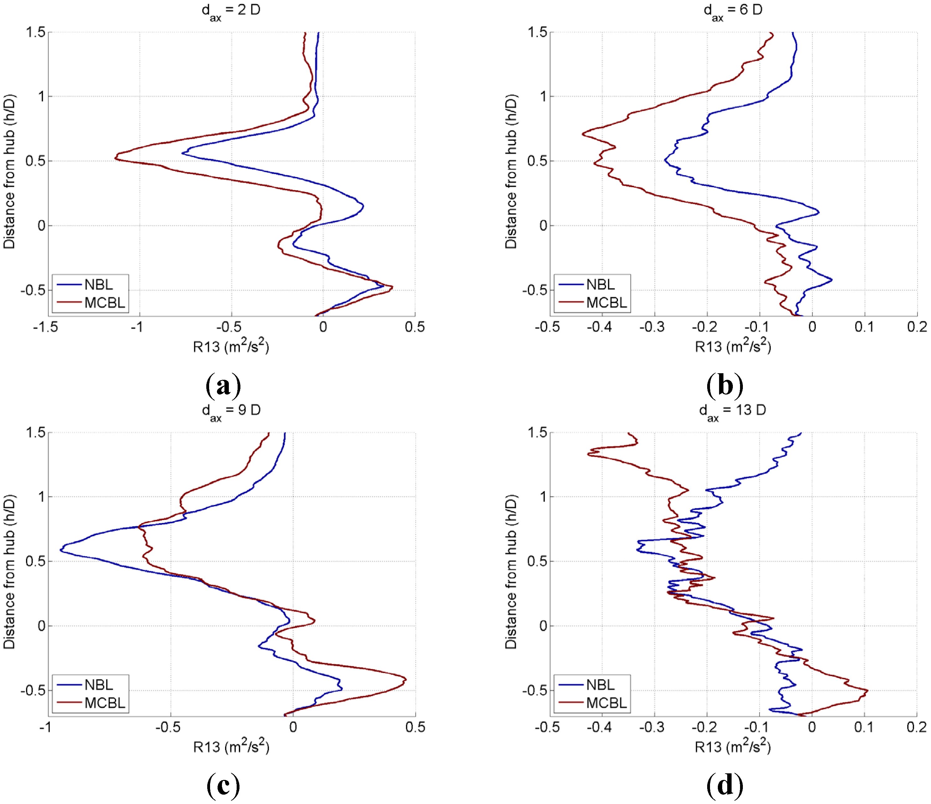
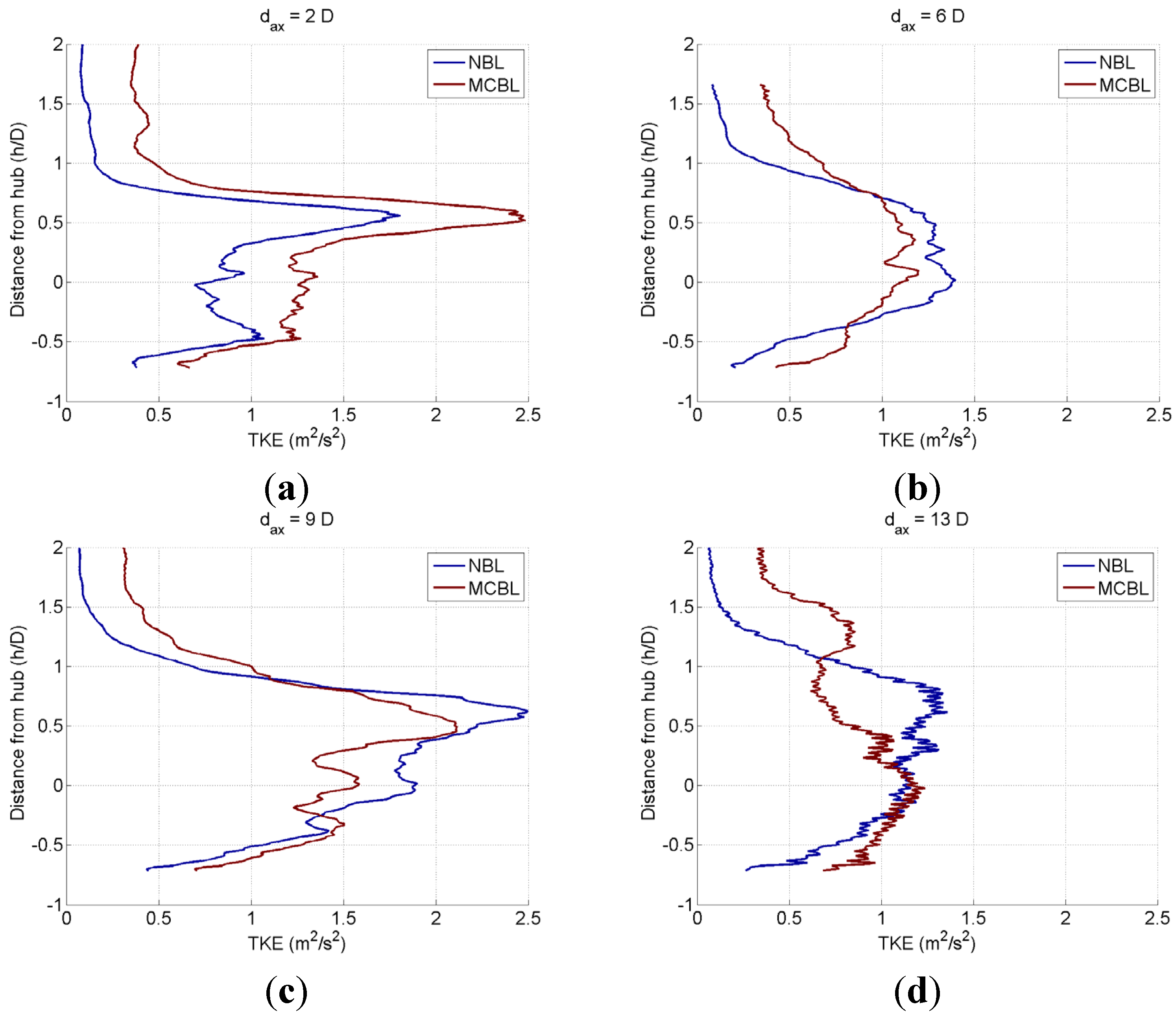
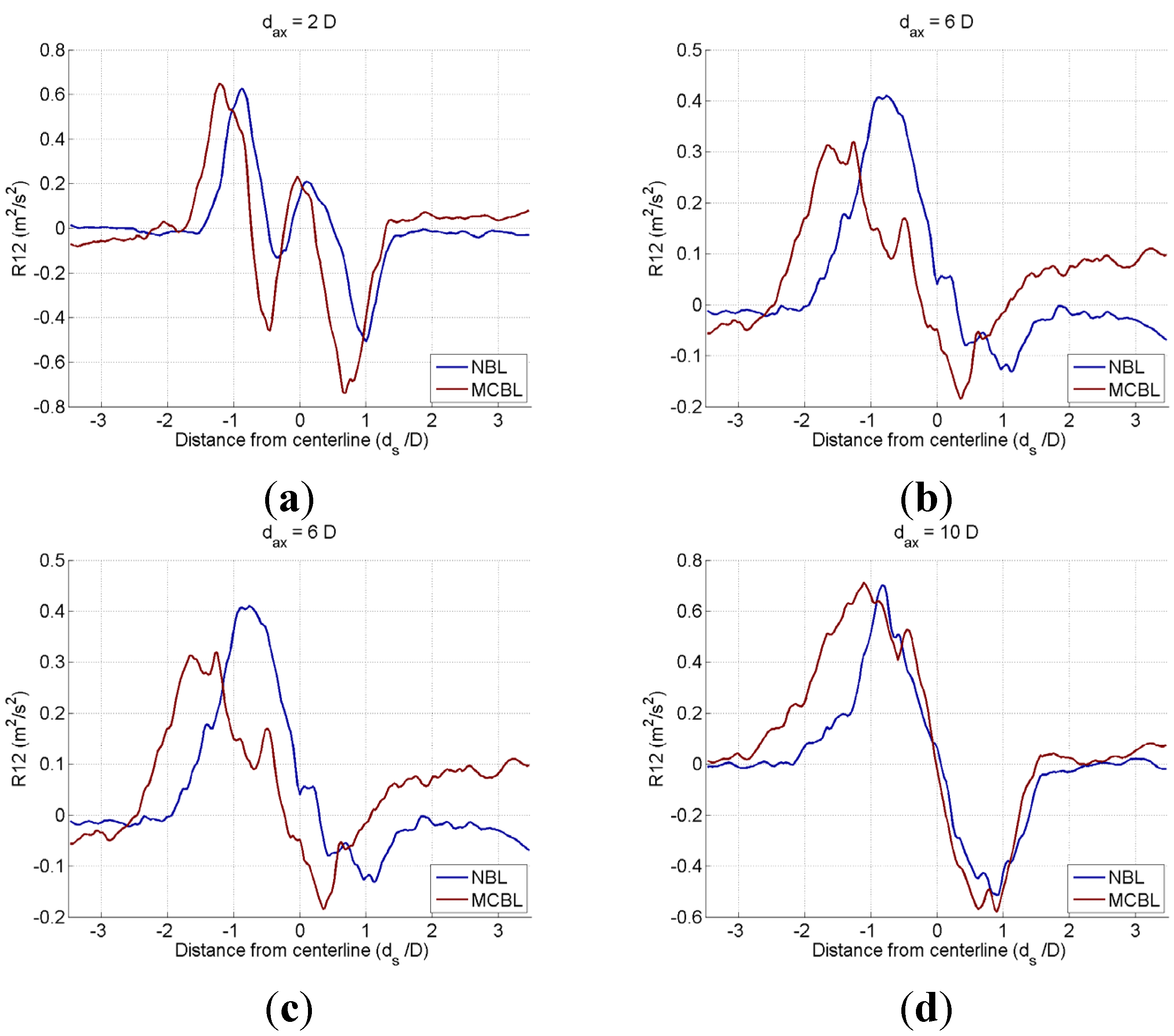
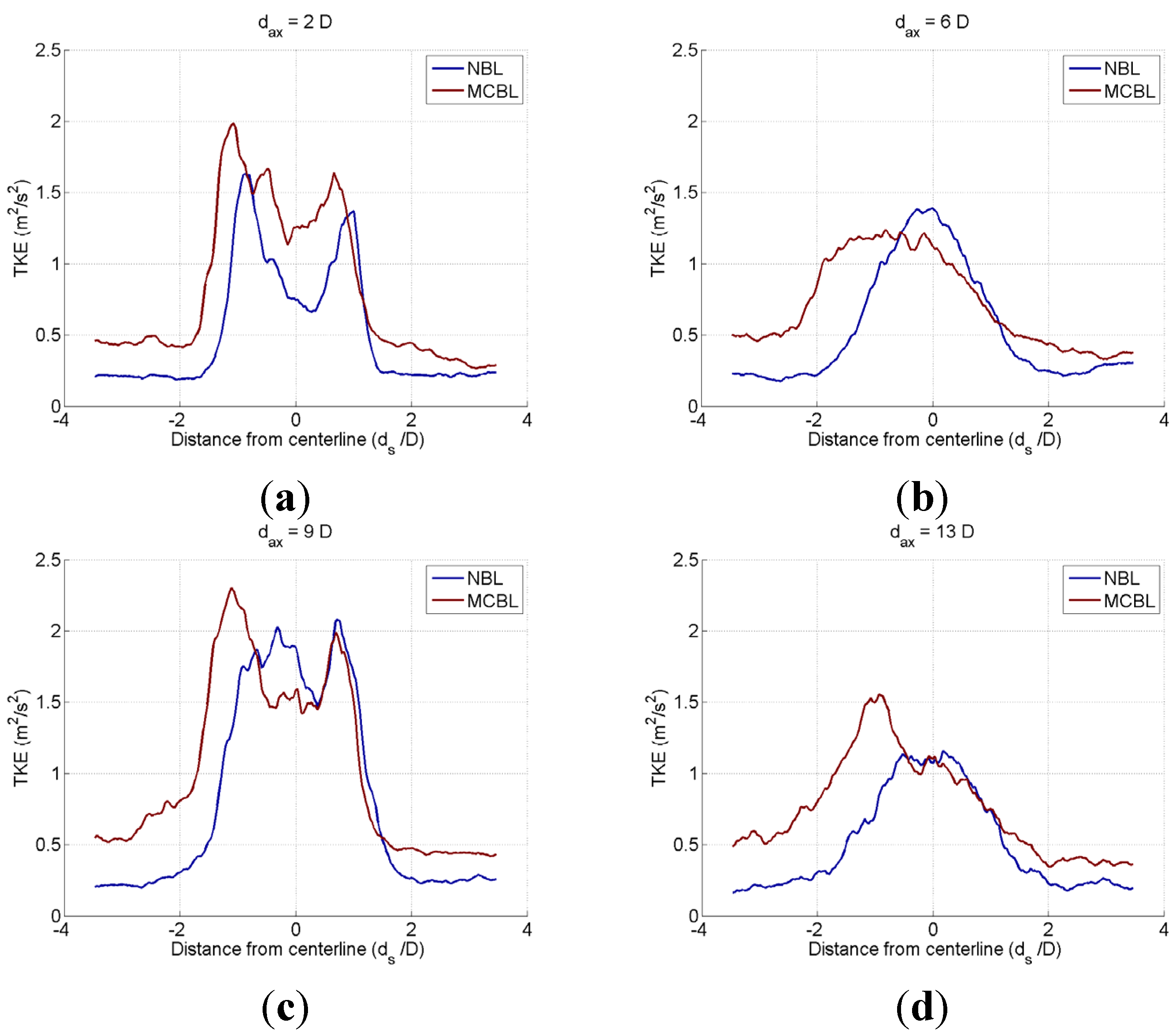
3.2.3. Wake Turbulence

In the previous section, the velocity deficit in the wake was presented. An attempt was made to understand the recovery pattern by considering the mean axial velocity. More physical insight into the process of wake recovery and turbulence transport can be gained by considering the correlation between fluctuations in different velocity components. The convention for describing the different velocity components is the following: The first is the axial velocity (U_axial or simply U). The second velocity component is positive along the rightward spanwise direction (when looking from a downstream location) and denoted by U_s (or V), and the third one is in the vertical direction and labeled as U_z (or W). The corresponding fluctuations are u’, v’, and w’. The Reynolds stress component, R₁₂, or the statistical correlation between u’ and v’, is an indicator of the meandering behavior of the wake; the correlation between u’ and w’, i.e., R₁₃, can be used to understand the entrainment from more energetic regions of the ABL above the turbine and wake region. This has been discussed extensively in the work by VerHulst and Meneveau [19]. The combined effect of the self-correlation of fluctuations in different velocity components (R_ii) is a proportional measure of the turbulent kinetic energy (TKE). As the wake grows, propagates, and decays downstream of a turbine, the turbulence level in the wake changes. The strengths of tip vortices and their breakdown, which depend on the ABL stability state, do affect the turbulence level in the wake.

Figure 11 shows the R₁₃ distribution along vertical lines for both stability states and at the same positions in the turbine wakes as the wake velocity distributions in Figure 10. Note that R₁₃ < 0 denotes turbulent momentum transport down to the surface. It is clear from Figure 11a,b that the MCBL case exhibits higher downward momentum transport than the NBL case, thus leading to faster wake recovery in Figure 10a,b and higher power for Turbine 2 in Figure 9a. The negative peak value for R₁₃ in Figure 11a,b occurs almost exactly at h/D = 0.5, i.e., the location of the upper blade.

Next, the TKE is studied along a vertical line (the same as used for the wake velocity deficit and Reynolds stress, R₁₃). Similar to Figure 11, the results are presented for 2D in Figure 12a,c and 6D in Figure 12b,d downstream of both turbines, and comparisons are made between the two ABL states, i.e., NBL and MCBL. As expected, the TKE is higher for the MCBL than for the NBL flow and 2D downstream of the first turbine in Figure 12a. It is interesting to note, though, that the TKE in the NBL grows at a higher rate in the turbine wakes than in the MCBL, as evidenced in Figure 12b–d. It can be observed that at 2D downstream of both turbines, Figure 12a,c, the peak TKE occurs at the upper edge of the wake at h/D = +0.5. At 6D downstream of both turbines in Figure 12b,d, the TKE distribution is more spread along the vertical lines. This can be attributed to wake rotation and ensuing turbulent mixing. The observation regarding peak TKE along vertical lines at different downstream locations is consistent with the flow field in an axial plane shown in Figure 6.

Figure 11. Reynolds stress R₁₃ distribution in the vertical direction. (Turbine-Turbine Interaction Problem, V_Wind = 8 m/s). (a) 2D downstream of Turbine 1; (b) 6D downstream of Turbine 1; (c) 2D downstream of Turbine 2; (d) 6D downstream of Turbine 2.

Figure 11. Reynolds stress R₁₃ distribution in the vertical direction. (Turbine-Turbine Interaction Problem, V_Wind = 8 m/s). (a) 2D downstream of Turbine 1; (b) 6D downstream of Turbine 1; (c) 2D downstream of Turbine 2; (d) 6D downstream of Turbine 2.

Figure 12. Turbulent Kinetic Energy (TKE) distribution in the vertical direction. (Turbine-Turbine Interaction Problem, V_Wind = 8 m/s). (a) 2D downstream of Turbine 1; (b) 6D downstream of Turbine 1; (c) 2D downstream of Turbine 2; (d) 6D downstream of Turbine 2.

Figure 12. Turbulent Kinetic Energy (TKE) distribution in the vertical direction. (Turbine-Turbine Interaction Problem, V_Wind = 8 m/s). (a) 2D downstream of Turbine 1; (b) 6D downstream of Turbine 1; (c) 2D downstream of Turbine 2; (d) 6D downstream of Turbine 2.

Figure 13 shows the R₁₂ distribution along a horizontal line at turbine hub height (or h/D = 0) for both stability states and at 2D and 6D downstream of both turbines. Note that R₁₂ > 0 for d_s/D < 0 and similarly R₁₂ < 0 for ds/D > 0 represent turbulent momentum transport into the rotor disk area. This can be indeed observed in Figure 13a. Of note is an apparent shift in R₁₂ to the left, signifying a meandering motion to that side over the averaging time interval of 1700 s. The sequence through Figure 13a–c further shows a reduction of inboard momentum transport for d_s/D > 0, which is attributed to the effective rotor disk area (and associated wake-induced turbulence) having meandered towards d_s/D < 0. It is worth mentioning that the positive and negative peaks in R₁₂ are again distributed more symmetrically 6D downstream of Turbine 2 in Figure 13d and similarly for both stability states. It appears that the combined wake of both turbines may have been sufficiently developed such that differences in inboard turbulent momentum transport through R₁₂ do not show significant differences between the two stability states; this is different, though, for the TKE level as shown in Figure 14d.

Figure 13. Reynolds stress R₁₂ distribution in the horizontal direction. (Turbine-Turbine Interaction Problem, V_Wind = 8 m/s). (a) 2D downstream of Turbine 1; (b) 6D downstream of Turbine 1; (c) 2D downstream of Turbine 2; (d) 6D downstream of Turbine 2.

Figure 13. Reynolds stress R₁₂ distribution in the horizontal direction. (Turbine-Turbine Interaction Problem, V_Wind = 8 m/s). (a) 2D downstream of Turbine 1; (b) 6D downstream of Turbine 1; (c) 2D downstream of Turbine 2; (d) 6D downstream of Turbine 2.

Figure 14. Turbulent Kinetic Energy (TKE) distribution in the spanwise direction at hub height. (Turbine-Turbine Interaction Problem, V_Wind = 8 m/s). (a) 2D downstream of Turbine 1; (b) 6D downstream of Turbine 1; (c) 2D downstream of Turbine 2; (d) 6D downstream of Turbine 2.

Figure 14. Turbulent Kinetic Energy (TKE) distribution in the spanwise direction at hub height. (Turbine-Turbine Interaction Problem, V_Wind = 8 m/s). (a) 2D downstream of Turbine 1; (b) 6D downstream of Turbine 1; (c) 2D downstream of Turbine 2; (d) 6D downstream of Turbine 2.

The meandering of the wake towards d_s/D < 0 is also evidenced by the shift (or asymmetry) of TKE concentration along the horizontal lines, as shown in Figure 14. This is consistent with the observation of iso-vorticity contours in Figure 5 and the discussion of R₁₂ stresses in Figure 13. The TKE peaks 2D downstream of both turbines in Figure 14a,c are associated with the blade tip vortices, with the MCBL case showing higher TKE in comparison to the NBL case. The d_s/D values of the TKE peaks in Figure 14a,c suggest wake expansion. The TKE peaks are not present 6D downstream of both turbines in Figure 14b,d, which is a strong indicator that the tip vortices have broken down in the wake. This is further substantiated by contours of iso-vorticity in Figure 5. Of further note in Figure 14b,d is that the MCBL case exhibits a wider TKE spread along the centerline at hub height than the NBL case. This is once more attributed to higher turbulence levels, see also I_h in Table 1.

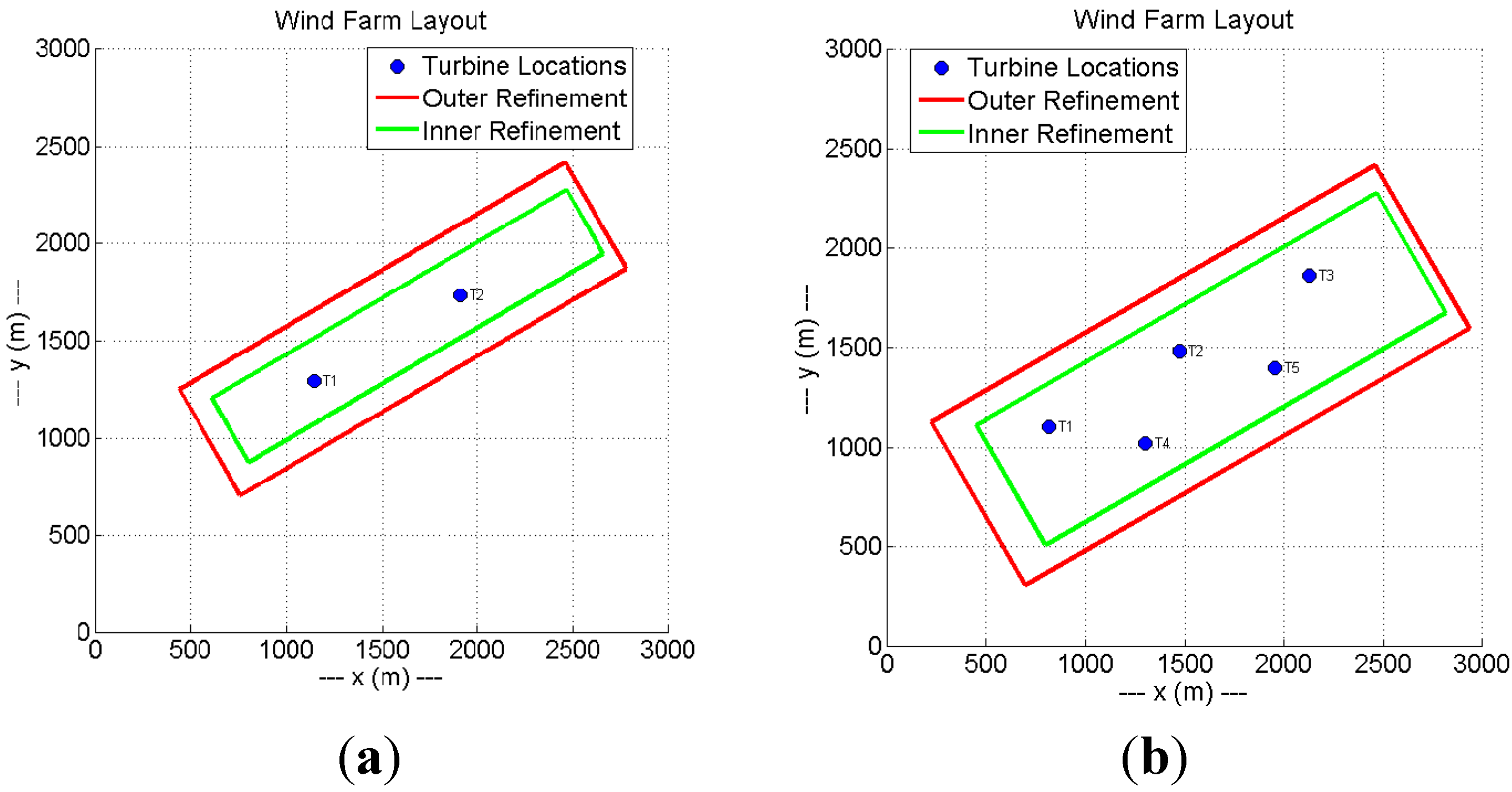
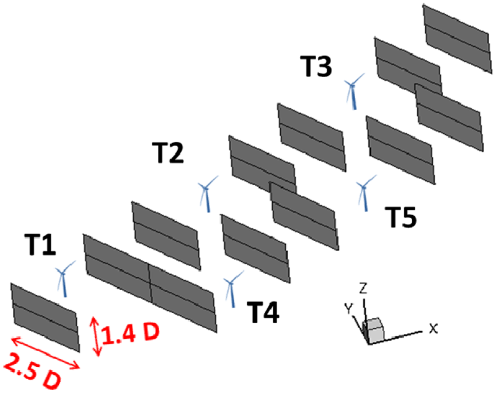
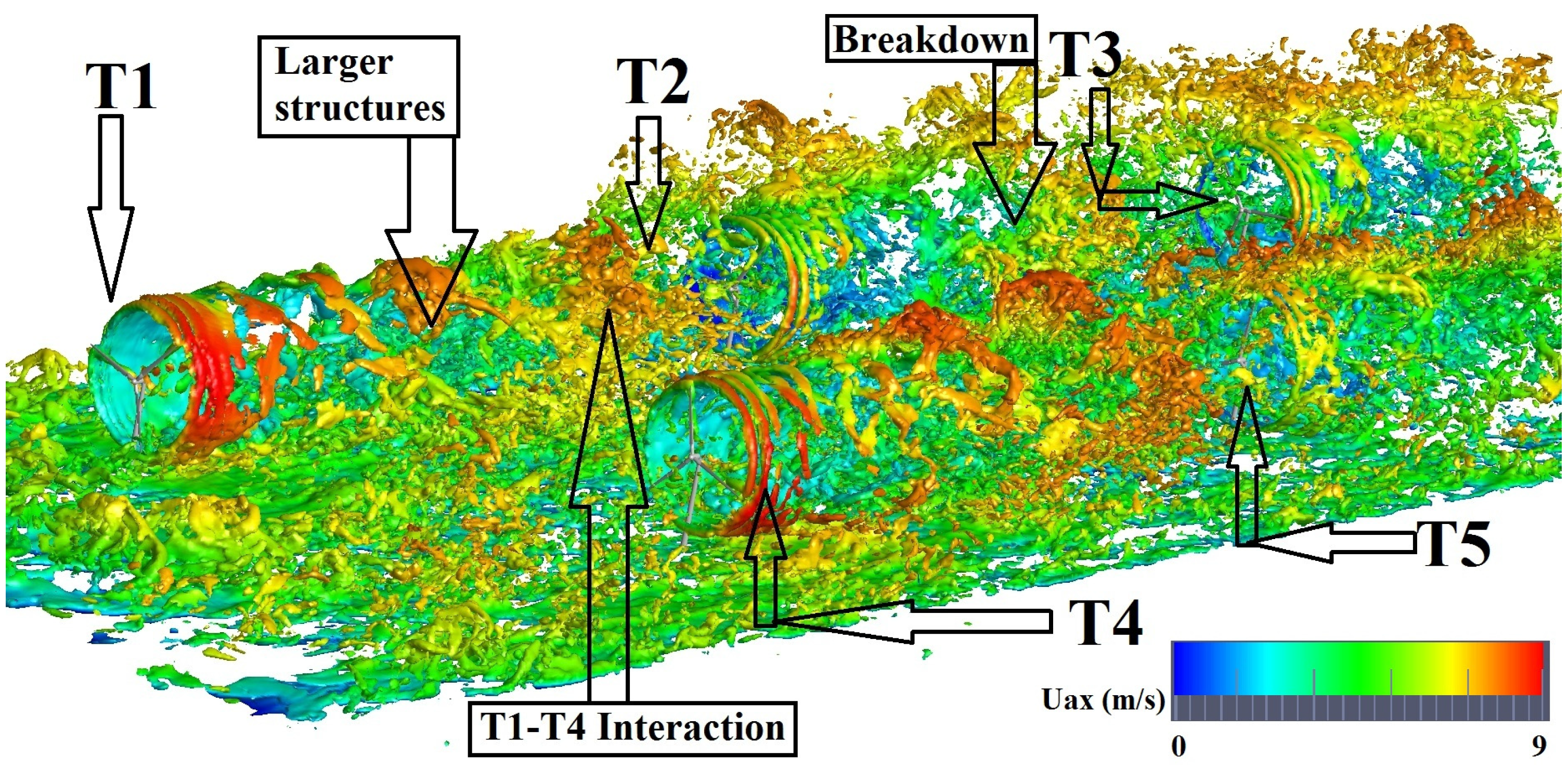
3.3. A Wind Farm Consisting of Five Wind Turbines (ALM OpenFOAM-LES)

For a conceptual array of five NREL 5-MW turbines, only MCBL inflow was considered. Here the main goal is to enhance the physical understanding that was obtained by the comparative study of the turbine-turbine interaction problem. The focus here is on understanding the mechanism of turbulence transport in a small wind farm rather than a comparison between stability states. For this study, two arrays, one consisting of three (upper or main diagonal, turbines numbered 1–3) and the other of two (lower or sub-diagonal, turbines numbered 4 and 5) NREL 5-MW wind turbines were considered in MCBL flow. Figure 3b shows the arrangement of the turbines in the wind farm. The turbine spacing is 6D within each array, and the 2-turbine (lower diagonal) array is staggered by 2.5D with respect to the other (upper diagonal) array.

Figure 15 shows an iso-surface of vorticity magnitude equal to 0.5 1/s colored by streamwise velocity. Similar to Figure 5 for the turbine-turbine interaction problem, it can be seen that tip vortices of downstream turbines break down faster than their upstream located counterparts. In addition, the coloring of the contours of iso-vorticity with the streamwise velocity reveals a lower advection velocity (higher wake deficit) at downstream turbines. It is also interesting to note that the upstream turbine in the lower array (Turbine 4) appears to be affected by the wake of the first turbine in the upper array (Turbine 1) in the sense that tip vortices break down faster and streamwise velocity appears to be lower at that particular instant in time.

Figure 15. Five-Turbine Wind Farm in MCBL flow (NREL 5-MW Turbines, V_Wind = 8 m/s).

Figure 15. Five-Turbine Wind Farm in MCBL flow (NREL 5-MW Turbines, V_Wind = 8 m/s).

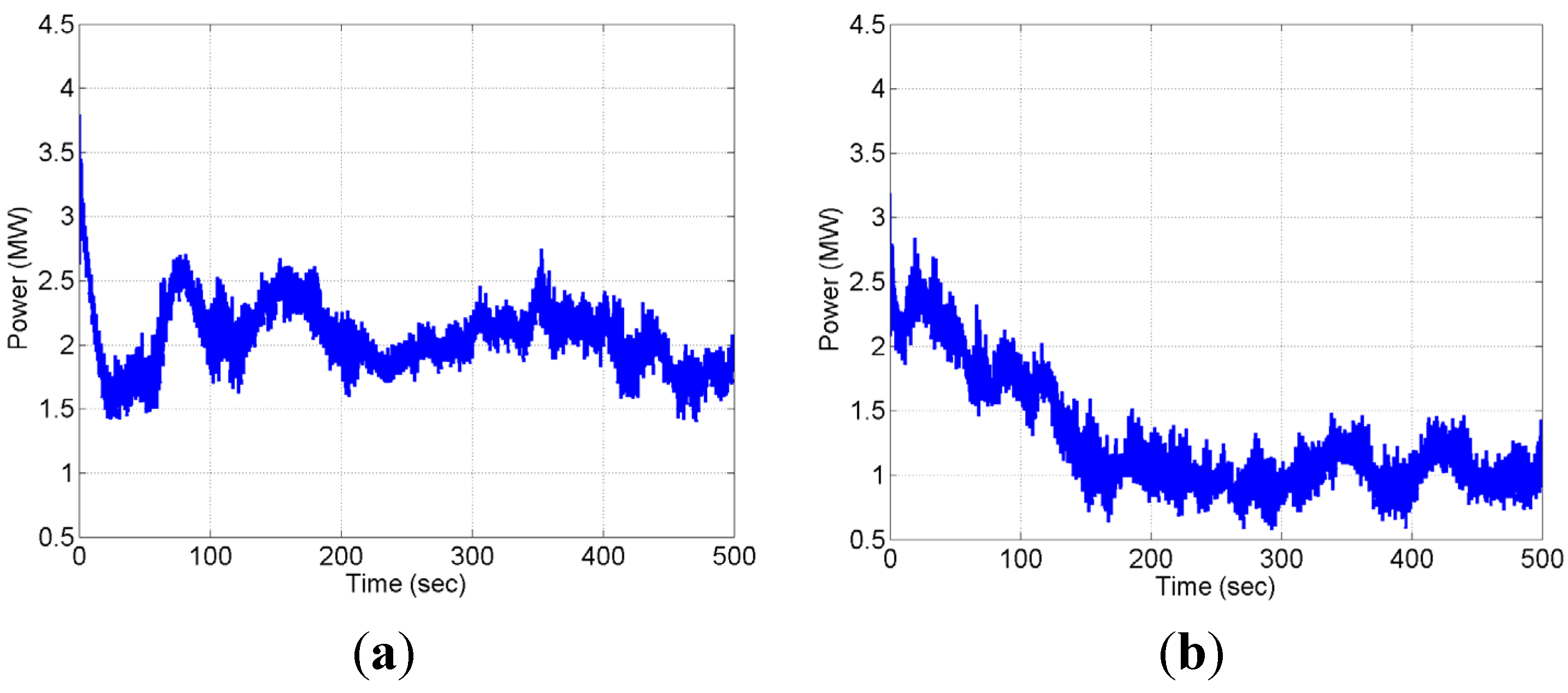
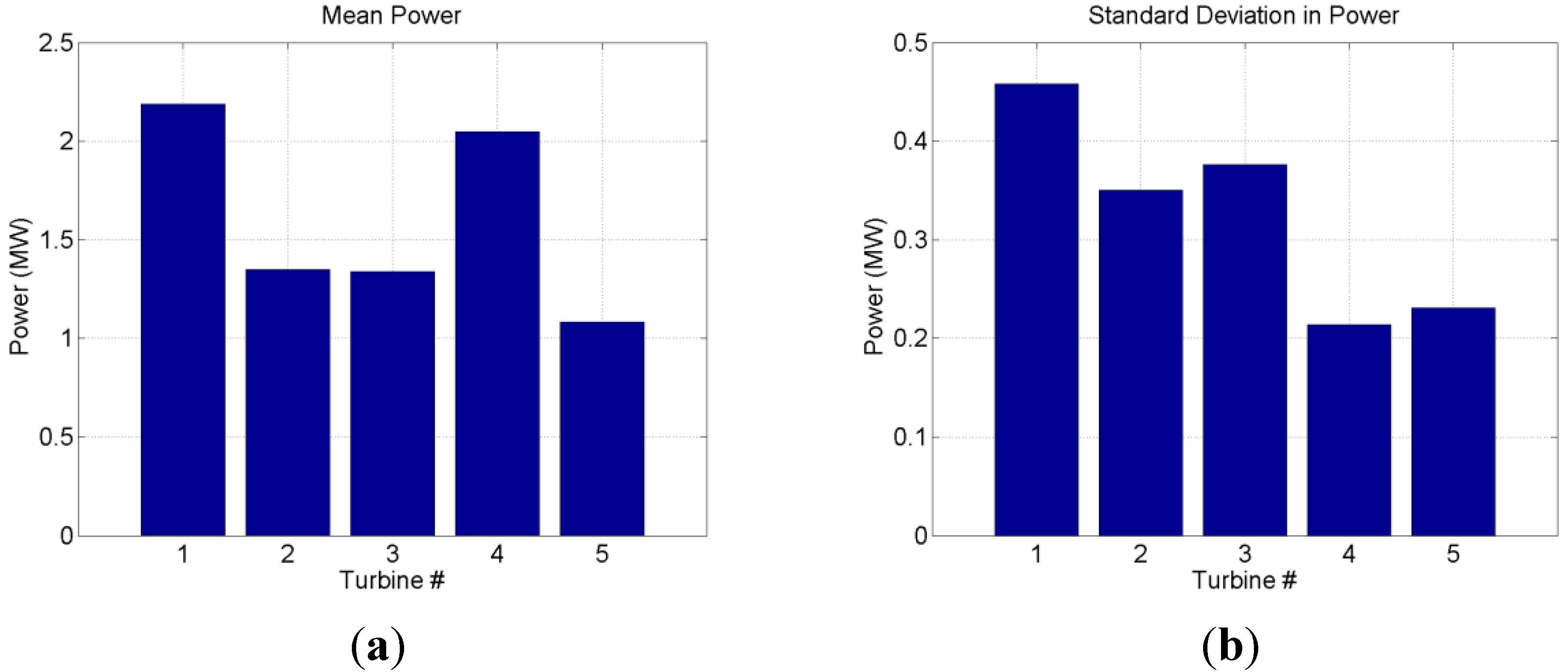
3.3.1. Turbine Power

The flow field for the five-turbine array in Figure 15 shows several structures that are expected to have impact on the blade loads and integrated power of the individual turbines. Here we study the integrated power, which is the combined effect of spanwise blade loads. The time series of turbine power up to 500 s of real time are shown in Figure 16 and Figure 17. For all downstream located turbines (Turbines 2 and 3 in the main diagonal and Turbine 5 in the sub-diagonal), the wakes of upstream turbines take approximately 150 s to reach the downstream turbines and interact with the former, Turbines 1 and 4 respectively. It should be noted that this time is less than that for NBL flow because of faster wake recovery. For Turbine 1, part of a large low-speed eddy of time scale t* in Table 1 passes through the rotor disk between 200 s and 300 s. The power loss within the upper array (main diagonal) is apparent from Figure 16b,c. The power suffers a dip at around 150 s when the wake from the upstream turbine starts affecting the former. Furthermore, it can be seen that Turbines 2 and 3 appear to have similar mean power. This is further substantiated in Figure 18, which shows the mean and standard deviation in power from 150 s to 500 s. It is also interesting to observe in Figure 16 how a portion of the low-speed eddy passing through Turbine 1 between 200 s and 300 s affects Turbine 2 at approximately 350 s and Turbine 3 around 400 s. The dip in power of Turbine 3 is due to the combined effects of wakes from Turbines 1 and 2 and the large eddy due to atmospheric turbulence. These correlations can be of importance for future strategies in controlling wind farms as the apparent eddy passage through Turbine 1 can be detected on time to alleviate some of the additional power drop in Turbines 2 and 3. As for the lower array (sub-diagonal) of turbines in Figure 17, it is interesting to note that the time series of power is overall less fluctuating than in the upper array in Figure 16. This can be attributed to the possibility that the sub-diagonal does not interact with the same low-speed atmospheric eddy.

Figure 16. Time series of turbine power (5-Turbine Wind Farm, V_Wind = 8 m/s). (a) Turbine 1; (b) Turbine 2; (c) Turbine 3.

Figure 16. Time series of turbine power (5-Turbine Wind Farm, V_Wind = 8 m/s). (a) Turbine 1; (b) Turbine 2; (c) Turbine 3.

Figure 17. Time series of turbine power (5-Turbine Wind Farm, V_Wind = 8 m/s). (a) Turbine 4; (b) Turbine 5.

Figure 17. Time series of turbine power (5-Turbine Wind Farm, V_Wind = 8 m/s). (a) Turbine 4; (b) Turbine 5.

Figure 18. Mean and standard deviation of turbine power (5-Turbine Wind Farm, V_Wind = 8 m/s). (a) Mean; (b) Std. Deviation.

Figure 18. Mean and standard deviation of turbine power (5-Turbine Wind Farm, V_Wind = 8 m/s). (a) Mean; (b) Std. Deviation.

Figure 18 shows the mean and standard deviation in turbine power for the 5-turbine array. It can be seen in Figure 18a that the power has leveled at Turbine 3 in the main diagonal. This is a typical behavior observed in many wind farms to date and one of the remaining “mysteries”. As far as the sub-diagonal (Turbines 4 and 5) is concerned, the staggered arrangement with respect to the main diagonal supports the hypothesis that the wake of Turbine 1, which is more upstream, does affect the power production of a staggered downstream array of wind turbines. Indeed, Turbines 4 and 5 produce less power than Turbines 1 and 2; however, a relatively larger drop can be seen in the standard deviation of turbine power in Figure 18b. Here it is apparent that power fluctuations are less for Turbines 4 and 5 (sub-diagonal) than for Turbines 1–3 (main diagonal). This is consistent with the time series of turbine power in Figure 16 and Figure 17. This suggests that there may be an adverse effect in mean power when staggering turbine arrays too close to one another. The smaller fluctuations (or standard deviation) are likely because of different eddying structures interacting with the sub-diagonal, and this can be substantiated only by further correlation between the passage of atmospheric eddies through the wind farm and the time series of power beyond the recorded 500 s of real time.

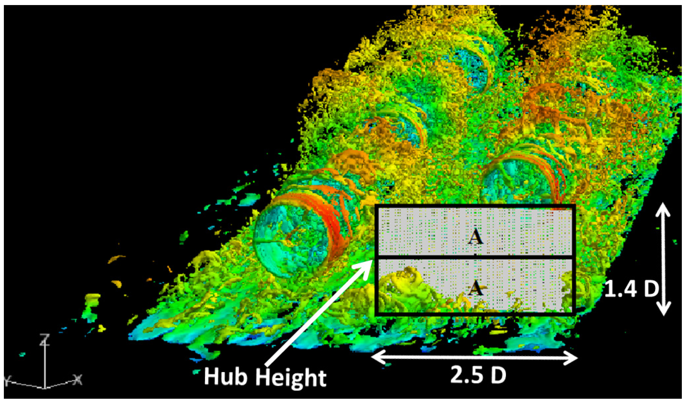
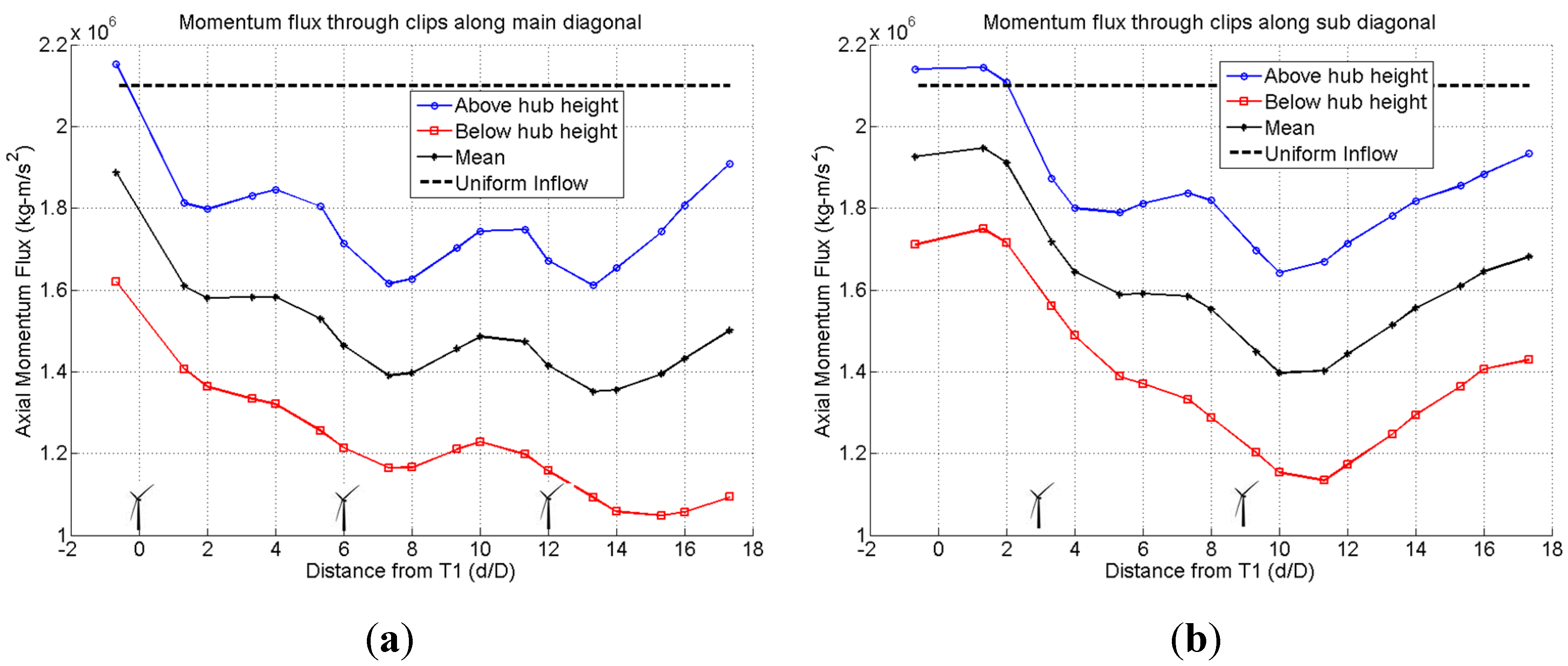
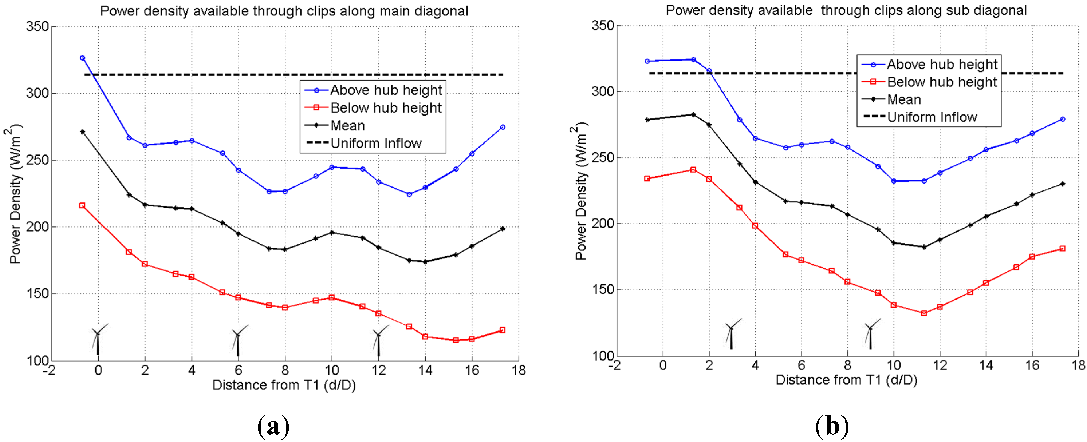
3.3.2. Dynamic Surface Clipping for Flux Analysis

As described in Section 3.2.3., correlations resulting from distributions of Reynolds stresses and TKE are useful in providing directional information on momentum transport and wake meandering; however, they do not provide integral values of total fluxes needed to quantify the subtleties of observed phenomena in the wake recovery process. It is here that the “Dynamic Surface Clipping” feature in FieldView enables efficient data extractions on surface planes combined with integrative post-processing methods. Figure 19 shows one of the extracted planar surfaces upstream of Turbine 4 in the sub-diagonal after “dynamic clipping” was applied. All “clipped” surface integration cutting planes are 2.5D wide and 1.4D high, allowing for equal areas, A, above/below turbine hub height at 0.7D. Figure 20 shows more examples of “clipped” surface integration cutting planes orthogonal to the primary flow direction. A total of 18 wake cutting planes were used in both the main diagonal and sub-diagonal of the considered 5-Turbine wind farm; not all are shown in Figure 20 for clarity.

Figure 19. Example of “clipped” integration surface cutting plane. (Cutting plane is divided into equal areas, A, above/below hub height).

Figure 19. Example of “clipped” integration surface cutting plane. (Cutting plane is divided into equal areas, A, above/below hub height).

Figure 20. Locations of “clipped” integration surface cutting planes in 5-Turbine Wind Farm. (For clarity, not all integration planes are shown).

Figure 20. Locations of “clipped” integration surface cutting planes in 5-Turbine Wind Farm. (For clarity, not all integration planes are shown).

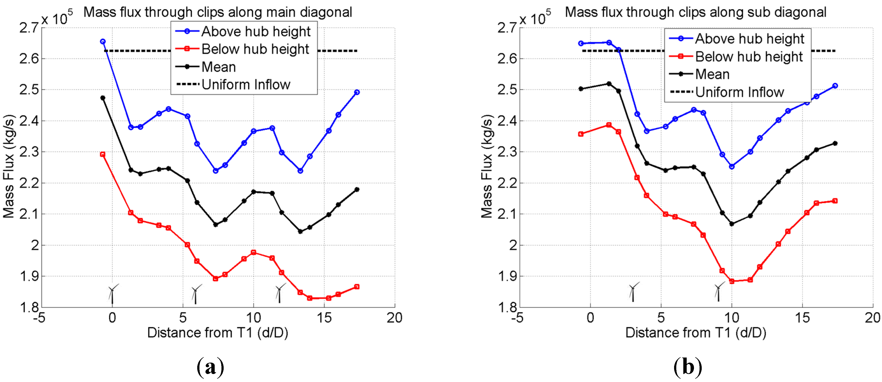
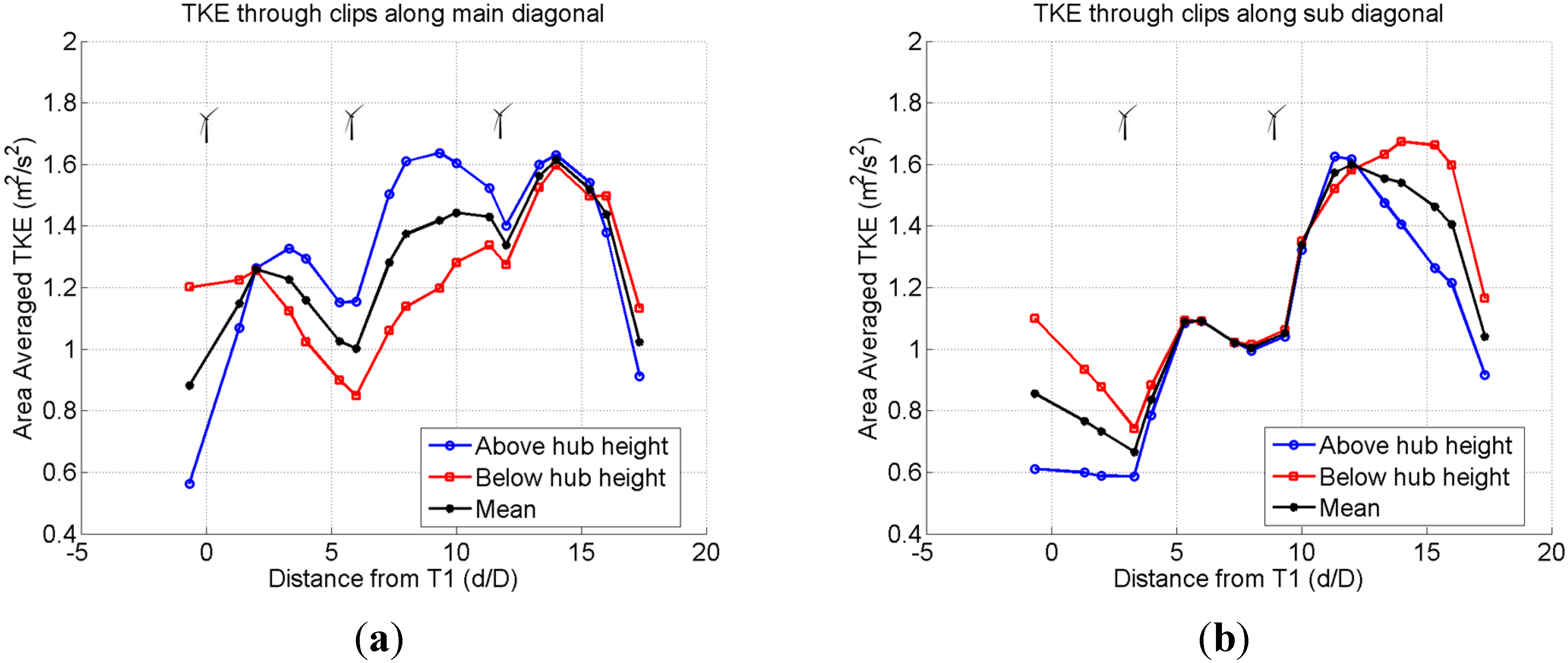
3.3.3. Integrated Quantities along “Dynamic Surface Clips” of Wake Surface Cutting Planes

Detailed analyses of mass and momentum fluxes, power density, and TKE were integrated along a total of 18 wake surface cutting planes along both the main diagonal (3-Turbine array) and sub-diagonal (2-Turbine array). Data were extracted for 10 rotor revolutions using the approach described for XDB workflow (Section 2.4). In addition, all wake surface cutting planes were split at turbine hub height into equal areas, A, to quantify separately the various integrated quantities above and below turbine hub height. Integrated fluxes are shown in Figure 21, Figure 22, Figure 23 and Figure 24 with the respective flux integral equations. By integrating mass and momentum fluxes as well as power density and TKE over these wake surface cutting planes, the mechanisms of the wake recovery process can be better understood. Figure 21, Figure 22, Figure 23 and Figure 24 below present integrations along the wake surface cutting planes for the different quantities and above hub height, below hub height, the mean of the two, and for uniform flow, with reference to the reference wind speed at hub height.

Figure 21. Mass flux across clipped wake surface cutting planes above/below hub height. (5-Turbine Wind Farm, V_Wind = 8 m/s). (a) Main diagonal (T1–T3); (b) Sub-diagonal (T4–T5). $MassFlux\dot{m}={\displaystyle \underset{A}{\iint }\mathrm{\rho }\overrightarrow{U}\cdot \overrightarrow{n}\text{ d}A}$.

Figure 21. Mass flux across clipped wake surface cutting planes above/below hub height. (5-Turbine Wind Farm, V_Wind = 8 m/s). (a) Main diagonal (T1–T3); (b) Sub-diagonal (T4–T5). $MassFlux\dot{m}={\displaystyle \underset{A}{\iint }\mathrm{\rho }\overrightarrow{U}\cdot \overrightarrow{n}\text{ d}A}$.

Figure 22. Momentum flux across clipped wake surface cutting planes above/below hub height. (5-Turbine Wind Farm, V_Wind = 8 m/s). (a) Main diagonal (T1–T3); (b) Sub-diagonal (T4–T5). $MomentumFlux\dot{p}={\displaystyle \underset{A}{\iint }(\mathrm{\rho }\overrightarrow{U})\overrightarrow{U}\cdot \overrightarrow{n}\text{ d}A}$.

Figure 22. Momentum flux across clipped wake surface cutting planes above/below hub height. (5-Turbine Wind Farm, V_Wind = 8 m/s). (a) Main diagonal (T1–T3); (b) Sub-diagonal (T4–T5). $MomentumFlux\dot{p}={\displaystyle \underset{A}{\iint }(\mathrm{\rho }\overrightarrow{U})\overrightarrow{U}\cdot \overrightarrow{n}\text{ d}A}$.

Figure 23. Power density across clipped wake surface cutting planes above/below hub height. (5-Turbine Wind Farm, V_Wind = 8 m/s). (a) Main diagonal (T1–T3); (b) Sub-diagonal (T4–T5). $PowerDensityP=1/A{\displaystyle \underset{A}{\iint }1/2\text{ ρ (}\overrightarrow{U}\cdot \overrightarrow{n}{)}^3\text{ d}A}$.

Figure 23. Power density across clipped wake surface cutting planes above/below hub height. (5-Turbine Wind Farm, V_Wind = 8 m/s). (a) Main diagonal (T1–T3); (b) Sub-diagonal (T4–T5). $PowerDensityP=1/A{\displaystyle \underset{A}{\iint }1/2\text{ ρ (}\overrightarrow{U}\cdot \overrightarrow{n}{)}^3\text{ d}A}$.

Figure 24. Averaged TKE across clipped wake surface cutting planes above/below hub height. (5-Turbine Wind Farm, V_Wind = 8 m/s). (a) Main diagonal (T1–T3); (b) Sub-diagonal (T4–T5). $AreaAveragedTKETK{E}_{Avg}=1/A{\displaystyle \underset{A}{\iint }1/2{\text{ (u′}}^2+{\text{v′}}^2+{\text{w′}}^2\text{) d}A}$.

Figure 24. Averaged TKE across clipped wake surface cutting planes above/below hub height. (5-Turbine Wind Farm, V_Wind = 8 m/s). (a) Main diagonal (T1–T3); (b) Sub-diagonal (T4–T5). $AreaAveragedTKETK{E}_{Avg}=1/A{\displaystyle \underset{A}{\iint }1/2{\text{ (u′}}^2+{\text{v′}}^2+{\text{w′}}^2\text{) d}A}$.

Integrated mass flux averaged over 10 rotor revolutions is plotted in Figure 21 for both the main diagonal and sub-diagonal of the 5-turbine wind farm. Turbine locations are indicated in Figure 21 (0D, 6D, and 12D in the main diagonal; 3D and 9D in the sub-diagonal). As expected, the turbines reduce the mass flux through the wake surface cutting planes as momentum and energy are being extracted by the turbines. Here we can interpret the reduction in mass flux as an effective streamtube expansion with mass leaving to the sides and top, i.e., away from the clipped wake surface cutting planes under consideration. It can be seen in Figure 21 that the mass flux through the clipped wake surface cutting planes recovers with downstream distance. An interesting observation in Figure 21a is that the mass flux below hub height recovers very slowly downstream of Turbine 3 while, up to that point, the mass fluxes above/below hub height changed approximately by the same magnitude. This is consistent with the observation for wake velocity deficit presented in Figure 10. Downstream of Turbine 5 in Figure 21b, the recovery patterns for above and below hub height are similar, indicating that a two-turbine array and a three-turbine array have different recovery pattern over the 10 revolutions that have been considered.

Figure 22 shows the momentum flux across clipped wake surface cutting planes in the main diagonal and sub-diagonal. It can be observed that the momentum below hub height downstream of Turbine 1 in Figure 22a and downstream of Turbine 4 in Figure 22b does not recover but continues to decrease, while the corresponding momentum above hub height does recover. This changes, though, in both diagonals after the respective second turbine, i.e., the wake momentum deficit below hub height does not recover until after the second turbine in a respective array (here diagonal) of wind turbines. This is attributed to turbulent transport from the outer energetic ABL surface layer above the wind turbines that has not yet energized the rotor disk area below hub height.

This is a very interesting discovery in the complex wake physics pertinent to wind turbines in the atmosphere. It is further hypothesized that this behavior is a contributor to the observed fact that turbine power levels at the third turbine within an array, as shown in Figure 18a. The observation regarding the lagging of momentum recovery in the wake surface cutting planes below hub height and downstream of the first turbine in an array is further substantiated by analyzing the actual power density (W/m²) through different clipped wake surface cutting planes. This is presented in Figure 23. It is apparent that above hub height, the recovery in power density is fairly shallow after Turbine 1 in Figure 23a but progressively increases downstream of Turbine 2 and Turbine 3. This is similar in Figure 23b for the sub-diagonal array. This supports the thought that downward momentum transport into the rotor disk area requires a long spatial distance in the ABL to develop. Comparing Figure 23a,b, it can be seen that Figure 23b shows a nearly parallel recovery of power density after the second turbine in the sub-diagonal, while this is not the case for the main diagonal in Figure 23a. This might support an idea of not placing a third turbine in an array but instead letting the wake recover evenly for a longer distance before placing an additional turbine.

Figure 24 presents area averages of Turbulent Kinetic Energy (TKE) through the clipped wake surface cutting planes. The values shown in Figure 24 were averaged over 10 rotor revolutions. It is best to interpret the plots shown in Figure 24 by looking at the mean (black line) and differences between sub-areas above/below hub height. It is apparent that wind turbines add TKE to the flow field. Unlike the observation in Figure 21, Figure 22 and Figure 23, it is interesting to note, though, that the addition of TKE is similar above and below hub height, in contrast to the momentum recovery in Figure 23, for example. Furthermore, addition of TKE increases progressively for downstream turbines, though the peak values in Figure 24a,b are almost identical. This means that there seems to be a maximum TKE in a wind turbine array.

4. Conclusions

This work presented a number of turbulence phenomena in the wakes of wind turbines arranged in different arrays and subject to different ABL stability states. The actuator line method (ALM) was used in an ALM OpenFOAM-LES solver for all computations. The turbine model was that of the notional NREL 5-MW baseline turbine developed by NREL. The analyses included time series of turbine power, spectra of turbine power, wake momentum (velocity) deficits, Reynolds stresses and turbulent kinetic energy (TKE) signifying wake turbulence and wake meandering, and integrated surface fluxes enabled through post-processing. The analyses presented in this work lead to the following conclusions:

• The ABL stability state defines the shear in the atmospheric boundary layer (ABL) and has a profound effect on the wake recovery and power production of wind turbine arrays.
• Array efficiency increases in a moderately-convective boundary layer (MCBL) compared to a neutral boundary layer (NBL), thus leading to a faster recovery of the wake momentum deficit. This is supported by R₁₃ distributions along vertical lines.
• Higher turbulence levels in MCBL compared to NBL conditions also lead to higher fatigue loads, in particular for the downstream turbine in a turbine-turbine interaction problem, as supported by higher standard deviation of turbine power.
• The peak TKE occurs at the upper edge of the wake and on the sides of the wake at hub height due to the presence of a developing shear layer and tip vortices.
• The shear due to the wake is far more pronounced than the shear due to ABL.
• The TKE distribution is broadened due to wake rotation and ensuing turbulent mixing.
• For wind farms arranged in staggered arrays, the downstream array is affected by the wake of the upstream array, even for perfectly aligned wind conditions (zero yaw). This leads to a small power loss in the (downstream) staggered array; however, the standard deviation in power, and most probably fatigue loads, are reduced at a higher rate compared to the power loss. This may be of interest for future array planning.
• The observed fact from many wind farms that power production has leveled out by the third turbine in an array has been confirmed in the computations of this work in the example of a 5-turbine wind farm.
• The use of the “dynamic surface clipping” method in FieldView allowed to separate integrated fluxes of mass, momentum, power density, and TKE in wake surface cutting planes above and below hub height. It was discovered that the lower portion of a wake surface cutting plane lags in its recovery process by about one turbine spacing.

There are still many questions that are unanswered about the complex flow physics in atmospheric flows and their interaction with wind turbines. This work showed how state-of-the-art flow visualization combined with quantitative analyses is a promising means of unraveling the remaining mysteries of wind turbine wakes.

References

1. Sørensen, J.N.; Shen, W.Z. Numerical modeling of Wind Turbine Wakes. ASME J. Fluids Eng. 2002, 124, 393–399. [Google Scholar] [CrossRef]
2. Troldborg, N.; Sørensen, J.N.; Mikkelsen, R. Actuator Line Simulation of Wake of Wind Turbine Operating in Turbulent Inflow. In Journal of Physics: Conference Series, The Science of Making Torque from Wind; Technical University of Denmark: Lyngby, Denmark, 2007. [Google Scholar]
3. Troldborg, N. Actuator Line Modeling of Wind Turbine Wakes. Ph.D. Thesis, Technical University of Denmark, Copenhagen, Denmark, 2008. [Google Scholar]
4. Troldborg, N.; Sørensen, J.; Mikkelsen, R. Numerical Simulations of Wake Characteristics of a Wind Turbine in Uniform Flow. Wind Energy 2010, 13, 86–99. [Google Scholar] [CrossRef]
5. Jensen, L.E. Array Efficiency at Horns Rev and the Effect of Atmospheric Stability. In Proceedings of the 2007 European Wind Energy Conference, Milan, Italy, 7–10 May 2007.
6. Rathmann, O.; Frandsen, S.T.; Barthelmie, R.J. Wake Modelling for Intermediate and Large Wind Farms. In Proceedings of the European Wind Energy Conference and Exhibition, Milan, Italy, 7–10 May 2007.
7. Churchfield, M.J.; Moriarty, P.J.; Vijayakumar, G.; Brasseur, J.G. Wind Energy-Related Atmospheric Boundary-Layer Large-Eddy Simulation Using OpenFOAM; National Renewable Energy Laboratory: Golden, CO, USA, 2010; NREL/CP-500–48905. [Google Scholar]
8. Churchfield, M.J. Wind Energy/Atmospheric Boundary Layer Tools and Tutorials. In Training Session at the 6th OpenFOAM Workshop; The Pennsylvania State University: University Park, PA, USA, 2011. [Google Scholar]
9. Churchfield, M.J.; Lee, S.; Moriarty, P.J.; Martínez, L.A.; Leonardi, S.; Vijayakumar, G.; Brasseur, J.G. A Large-Eddy Simulation of Wind-Plant Aerodynamics. In Proceedings of the 50th AIAA Aerospace Sciences Meeting, Nashville, TN, USA, 9–12 January 2012.
10. Martínez, L.A.; Leonardi, S.; Churchfield, M.J.; Moriarty, P.J. A Comparison of Actuator Disk and Actuator Line Wind Turbine Models and Best Practices for Their Use. In Proceedings of the 50th AIAA Aerospace Sciences Meeting, Nashville, TN, USA, 9–12 January 2012.
11. Churchfield, M.J.; Lee, S.; Michalakes, J.; Moriarty, P.J. A Numerical Study of the Effects of Atmospheric and Wake Turbulence on Wind Turbine Dynamics. J. Turbul. 2012, 13, 1–32. [Google Scholar]
12. Jha, P.K.; Churchfield, M.J.; Moriarty, P.J.; Schmitz, S. Accuracy of State-of-the-Art Actuator-Line Modeling for Wind Turbine Wakes. In Proceedings of the 51th AIAA Aerospace Sciences Meeting, Grapevine, TX, USA, 7–10 January 2013.
13. Jha, P.K.; Churchfield, M.J.; Moriarty, P.J.; Schmitz, S. Guidelines for Volume Force Distributions within Actuator Line Modeling of Wind Turbines on Large-Eddy Simulation-type Grids. ASME J. Sol. Energy Eng. 2014, 136. [Google Scholar] [CrossRef]
14. Jha, P.K.; Churchfield, M.J.; Moriarty, P.J.; Schmitz, S. The Effect of Various Actuator-Line Modeling Approaches on Turbine-Turbine Interactions and Wake-Turbulence Statistics in Atmospheric Boundary-Layer Flow. In Proceedings of the 52th AIAA Aerospace Sciences Meeting, National Harbor, MD, USA, 13–17 January 2014.
15. OpenFOAM, Ver. 2.0.x, ESI Group-OpenCFD. Available online: http://www.openfoam.org/git.php (accessed on 20 April 2015).
16. Porté-Agel, F.; Wu, Y.; Chen, C. A Numerical Study of the Effects of Wind Direction on Turbine Wakes and Power Losses in a Large Wind Farm. Energies 2013, 6, 5297–5313. [Google Scholar] [CrossRef]
17. Wu, Y.; Porté-Agel, F. Atmospheric Turbulence Effects on Wind-Turbine Wakes: An LES Study. Energies 2012, 5, 5340–5362. [Google Scholar] [CrossRef]
18. Sim, C.; Basu, S.; Manuel, L. On Space-Time Resolution of Inflow Representations for Wind Turbine Loads Analysis. Energies 2012, 5, 2071–2092. [Google Scholar] [CrossRef]
19. VerHulst, C.; Meneveau, C. Altering Kinetic Energy Entrainment in Large Eddy Simulations of Large Wind Farms Using Unconventional Wind Turbine Actuator Forcing. Energies 2015, 8, 370–386. [Google Scholar] [CrossRef]
20. Bhaganagar, K.; Debnath, M. Implications of Stably Stratified Atmospheric Boundary Layer Turbulence on the Near-Wake Structure of Wind Turbines. Energies 2014, 7, 5740–5763. [Google Scholar] [CrossRef]
21. Bhaganagar, K.; Debnath, M. The effects of mean atmospheric forcings of the stable atmospheric boundary layer on wind turbine wake. J. Renew. Sustain. Energy 2015, 7. [Google Scholar] [CrossRef]
22. Chamorro, L.P.; Porté-Agel, F. Turbulent Flow Inside and Above a Wind Farm: A Wind-Tunnel Study. Energies 2011, 4, 1916–1936. [Google Scholar] [CrossRef]
23. Chamorro, L.P.; Arndt, R.E.A.; Sotiropoulos, F. Turbulent Flow Properties Around a Staggered Wind Farm. Bound. Layer Meteorol. 2011, 141, 349–367. [Google Scholar] [CrossRef]
24. Chamorro, L.P.; Arndt, R.E.A.; Sotiropoulos, F. Reynolds number dependence of turbulence statistics in the wake of wind turbines. Wind Energy 2012, 15, 733–742. [Google Scholar] [CrossRef]
25. Sørensen, J.N.; Mikkelsen, R.F.; Henningson, D.S.; Ivanell, S.; Sarmast, S.; Andersen, S.J. Simulation of wind turbine wakes using the actuator line technique. Phil. Trans. R. Soc. A 2014, 373. [Google Scholar] [CrossRef] [PubMed]
26. Smagorinsky, J. General circulation experiments with the primitive equations. Mon. Weather Rev. 1963, 91, 99–164. [Google Scholar] [CrossRef]
27. Rhie, C.M.; Chow, W.L. Numerical Study of the Turbulent Flow Past an Airfoil with Trailing Edge Separation. AIAA J. 1983, 21, 1525–1532. [Google Scholar] [CrossRef]
28. Issa, R.I. Solution of the Implicitly Discretized Fluid Flow Equations by Operator-Splitting. J. Comput. Phys. 1985, 62, 40–65. [Google Scholar] [CrossRef]
29. Intelligent Light. Available online: http://www.ilight.com (accessed on 20 April 2015).
30. Bashioum, J.L.; Jha, P.K.; Schmitz, S.; Duque, E.P.N. Wake Turbulence of Two NREL 5-MW Wind Turbines Immersed in a Neutral Atmospheric Boundary-Layer Flow. American Physical Society Division of Fluid Dynamics. Available online: http://arxiv.org/abs/1310.3294 (accessed on 15 October 2013).
31. Stull, R.B. Meteorology for Scientists and Engineers, 2nd ed.; Brooks/Cole: Florence, KY, USA, 2000. [Google Scholar]
32. Jonkman, J.; Butterfield, S.; Musial, W.; Scott, G. Definition of a 5-MW Reference Wind Turbine for Offshore System Development; NREL-TP-500–38060; National Renewable Energy Laboratory (NREL): Golden, CO, USA, 2009. [Google Scholar]
33. Lee, S.; Churchfield, M.J.; Moriarty, P.J.; Jonkman, J.; Michalakes, J. A Numerical Study of Atmospheric and Wake Turbulence Impacts on Wind Turbine Fatigue Loadings. ASME J. Sol. Energy Eng. 2013, 135. [Google Scholar] [CrossRef]
34. Vijayakumar, G.; Brasseur, J.G.; Lavely, A.W.; Kinzel, M.P.; Paterson, E.G.; Churchfield, M.J.; Moriarty, P.J. Considerations in coupling LES of the atmosphere to CFD around wind turbines. In Proceedings of the 50th AIAA Aerospace Sciences Meeting, Nashville, TN, USA, 9–12 January 2012.
35. Lavely, A.W.; Vijayakumar, G.; Brasseur, J.G.; Paterson, E.G.; Kinzel, M.P. Comparing Unsteady Loadings on Wind Turbines using TurbSim and LES Flow Fields. In Proceedings of the 50th AIAA Aerospace Sciences Meeting, Nashville, TN, USA, 9–12 January 2012.