Co-Production of Olefins, Fuels, and Electricity from Conventional Pipeline Gas and Shale Gas with Near-Zero CO₂ Emissions. Part II: Economic Performance

Abstract

In this paper, techno-economic analyses of a polygeneration system for the production of olefins, transportation fuels and electricity are performed, considering various process options. Derivative-free optimization algorithms were coupled with Aspen Plus simulation models to determine the optimum product portfolio as a function of a wide variety of market prices. The optimization results show that the proposed plant is capable of producing olefins with the same production costs as traditional petrochemical routes while having effectively zero process CO₂ emissions (including the utilities). This provides an economic and more sustainable alternative to traditional naphtha cracking.

1. Introduction

The production of olefins from methanol, called methanol-to-olefins (MTO), is a novel process concept that can produce petrochemical feedstocks from alternative fuels [1]. Therefore, it can be an interesting option to meet global demand for petrochemical feedstocks, which is growing relatively steadily [2]. In addition, by incorporation of advanced CO₂ capture systems, the MTO process can also diminish the carbon emissions of petrochemical industries by replacing traditional steam cracking units [3].

The MTO process can be improved by incorporating it into a polygeneration process, in which other products are co-produced. By tightly integrating the different parts of the polygeneration process together, significant profitability and efficiency improvements can result [4,5,6]. Several studies have been performed on the techno-economic analysis of various polygeneration models. Most of these works focused on the hybrid systems that use multiple feedstocks such as coal and natural gas [7,8], coal and biomass [9], or coal and oven gas [10], for the co-production of transportation fuels, methanol, hydrogen and power. However, none of these works considered the impact of incorporating innovative CO₂ capture technologies such as oxy-fuel combustion and chemical looping combustion processes.

The main objective of this work is techno-economic optimization of a novel polygeneration process that co-produces methanol, liquid transportation fuel (dimethyl ether), and olefins from natural gas. The economic performance of different advanced power generation options are studied in this paper: chemical looping combustion using nickel oxide, iron oxide, oxyfuel combustion, and conventional combustion with a gas turbine. The economic optimization also included investigating the impact of the feedstock composition by considering conventional natural gas as well as different types of shale gas. Details of the impact of gas composition on the plant’s configuration and geographic location are described in part I of this work.

In this paper, optimization algorithms were used in an economic analysis to determine the highest profitability for each design variant, or the highest production rate of olefins (both are considered as separate objective functions in separate optimization problems), considering a selected subset of the most important design parameters. Because market conditions are always subject to change, this was repeated for a wide variety of market conditions, ranging from low to high prices for the various products generated in each process. Finally, the most promising variants of the MTO concept were compared to naphtha cracking and ethane cracking processes for olefin production, the closest competing processes, showing promising results. The models used for each of the individual unit operations were either developed in the prior work of our group or other groups.

2. Economic Baseline

The profitability of each process was determined by computing the net present value (NPV) as the primary economic indicator. Capital costs were determined from published sources wherever possible, such as for the reformer section, MeOH synthesis section, power generation section and carbon sequestration units [7,11]. The capital costs of other units which did not have available cost data were estimated using the Aspen Icarus software package. This tool is commonly used to predict the capital cost of common chemical engineering unit operations and is updated regularly. In this work, it was used to predict the capital costs of individual unit operations such as pumps, compressors, and distillation columns which were not included in the sections listed previously. Table 1 lists all economic analysis parameters, market prices and assumptions for calculating the net present value (NPV) of all design cases, with citations to justify each parameter included in that table. Note that the utility and market prices shown are those used only for “base-case” calculations. Since prices vary from place to place and change somewhat unpredictably in the future, a sensitivity analysis which includes the effects of changes in price is discussed in Section 4. All financial parameters, such as interest rates, are chosen based on recommendations of prior work. Other business related expenses such as labor, overhead, laboratory operations, and maintenance are included using estimate formulas common to most analyses of this type. A detailed listing of the costs of each line item for each specific design option can be found in the supplementary material. Although all of these parameters can change from case to case, an extensive sensitivity analysis of all parameters considered is outside the scope of this work. However, even though there is uncertainty in the exact values of the NPV, the parameters are applied equally to all process variants and so meaningful conclusions can be made about the relative comparison of one process option to another.

Table 1. Base-case market prices and economic assumptions.

Feeds and Products	Market Prices
Natural gas & Ethane prices, $/MMBtu	3.88, [12]
NiO (commercial grade, 76% wt.), $/kg	20, [13]
NiO Disposal Cost, $/kg	5 (1)
NiO life span, h	10,000, [14]
Fe2O3 (commercial grade, 96% wt.), $/kg	1.44, [15]
Fe2O3 Disposal Cost, $/kg	0.36 (1)
Fe2O3 life span, h	3000, [16] (page 203)
Electricity, ¢/kWh	5.67, [17]
MeOH price, $/tonne	482, [18]
DME, $/tonne	962, [19]
Propylene, $/tonne	1340, [20]
Ethylene, $/tonne	1424, [21]
Economic Assumptions, [7,22 ]	Values
Plant capacity (shale gas inlet rate)	1111 MW, LHV
Operation time (h/year)	8760
Capacity factor	85%
Chemical engineering plant cost index	574.3, [23]
Plant lifetime (year)	30
Loan lifetime (year)	30
Interest rate on loan	9.5%
Debt percentage	50%
Inflation	2.79%
Federal + state tax rate	40%
Equity return rate	20%
NPV Calculation Elements, [22 ]	Values
Indirect cost	20% Fixed capital cost
Working capital cost	15% Total investment
Operating labor	10% Total production cost
Direct supervisory and clerical labor	10% Operating labour
Utilities	10% Total product cost
Maintenance and repairs	5% Fixed capital investment
Operating supplies	10% Maintenance and repair
Laboratory charges	10% Operating labour
Plant-overhead	50% of cost for operating labour, supervision, and maintenance
Administrative costs	15% of cost for operating labor, supervision, and maintenance
R&D, distribution and selling costs	4% of total product cost

⁽¹⁾ Due to lack of published data, assumed to be 25% of the metal-oxide price.

Table 1. Base-case market prices and economic assumptions.

Feeds and Products	Market Prices
Natural gas & Ethane prices, $/MMBtu	3.88, [12]
NiO (commercial grade, 76% wt.), $/kg	20, [13]
NiO Disposal Cost, $/kg	5 (1)
NiO life span, h	10,000, [14]
Fe2O3 (commercial grade, 96% wt.), $/kg	1.44, [15]
Fe2O3 Disposal Cost, $/kg	0.36 (1)
Fe2O3 life span, h	3000, [16] (page 203)
Electricity, ¢/kWh	5.67, [17]
MeOH price, $/tonne	482, [18]
DME, $/tonne	962, [19]
Propylene, $/tonne	1340, [20]
Ethylene, $/tonne	1424, [21]
Economic Assumptions, [7,22 ]	Values
Plant capacity (shale gas inlet rate)	1111 MW, LHV
Operation time (h/year)	8760
Capacity factor	85%
Chemical engineering plant cost index	574.3, [23]
Plant lifetime (year)	30
Loan lifetime (year)	30
Interest rate on loan	9.5%
Debt percentage	50%
Inflation	2.79%
Federal + state tax rate	40%
Equity return rate	20%
NPV Calculation Elements, [22 ]	Values
Indirect cost	20% Fixed capital cost
Working capital cost	15% Total investment
Operating labor	10% Total production cost
Direct supervisory and clerical labor	10% Operating labour
Utilities	10% Total product cost
Maintenance and repairs	5% Fixed capital investment
Operating supplies	10% Maintenance and repair
Laboratory charges	10% Operating labour
Plant-overhead	50% of cost for operating labour, supervision, and maintenance
Administrative costs	15% of cost for operating labor, supervision, and maintenance
R&D, distribution and selling costs	4% of total product cost

⁽¹⁾ Due to lack of published data, assumed to be 25% of the metal-oxide price.

Process Optimization

For each process variant, three design variables were subject to optimization, as noted in Figure 3 of part I of this study: the recycle ratio of unreacted gas sent to the MeOH reactor, the split ratio of MeOH which is sent to the MTO section (stream 2–7), and the split ratio of the MeOH stored as the final product (stream 2–8). Other process variables are adjusted to either meet the process constraints and product specifications, or selected based on suggested values in literatures. The feasibility range of all decision variables is fixed between 1% and 99%. Bounds of 0% and 100% were not used in order to avoid simulation problems in the software associated with zero flows. Instead, if the lower bound of 1% on a variable was reached, the simulation was reconstructed manually using 0% and adjusting the others proportionally (where in some cases the corresponding process section was eliminated), and if it improved the objective function, it was taken as the final result for that instance. A similar technique was used for 99%, which was reconstructed manually using 100%.

Because there were only three decision variables, a coarse-grain method (an exhaustive search over a grid) was used to sample the decision space in three dimensions for each design variant. For example, the effect of the recycle ratio and the ratio of MeOH to the MTO section are shown in Figure 1 for two different MeOH to MTO ratios. It can be seen that unlike the low olefin production ratio (Figure 1a), the optimum MeOH to DME ratio is between 20%–40% in the high olefin production scenario (Figure 1b). In addition, the influence of electricity, MeOH, DME and olefin market price fluctuations as a function of different process variables are depicted in Figure 2.

Figure 1. Effect of recycle ratio of unreacted gases to the methanol synthesis reactor and %MeOH to DME section on the NPV of plant at (a) low olefin (5%); (b) high olefin (50%) production ratios.

Figure 1. Effect of recycle ratio of unreacted gases to the methanol synthesis reactor and %MeOH to DME section on the NPV of plant at (a) low olefin (5%); (b) high olefin (50%) production ratios.

The sensitivity analysis shown in Figure 1 and Figure 2 illustrate the impact of the main three decision variables on the NPV of plant at different market prices. Due to the relative long run time required per simulation (approximately one minute), the spacing between sample points was too large to sufficiently locate an optimum in a reasonable amount of time. The built-in Aspen Plus optimization tool was also found to be insufficient and improved the results only trivially compared to the coarse-grain method, even when starting from a variety of different initial conditions.

Figure 2. The NPV of plant at different market prices and selected decision variables changes: (a) recycle ratio and Electricity price; (b) %MeOH to DME and MeOH price; (c) %MeOH to DME and DME price; (d) %MeOH to MTO and ethylene price.

Figure 2. The NPV of plant at different market prices and selected decision variables changes: (a) recycle ratio and Electricity price; (b) %MeOH to DME and MeOH price; (c) %MeOH to DME and DME price; (d) %MeOH to MTO and ethylene price.

Instead, three heuristic-based, derivative-free black box optimization algorithms were considered, namely particle swarm optimization, genetic algorithms, and simulated annealing. These are stochastic methods which use different strategies of exploring the decision variable space broadly at first and then later exploring promising subspaces in more and more depth. Eventually, the algorithms terminate once no more improvements can be found, and the best known point is usually locally optimal within tolerances, with a good chance that it is also the global optimal if the problem is not too “bumpy” and the heuristics were chosen correctly. Fortunately, finding the true optimum point is not critical to this work, and since the coarse-grain method samples points across the entire range of the state space, suboptimum results are expected to deviate from the true global optimum by only small amounts. These algorithms were implemented in Matlab and were coupled with the Aspen Plus simulations through the Excel interface. The three algorithms were used on a subset of cases to determine which derivative-free algorithm was the most promising. Standard algorithms have been used for each optimization technique and have not been detailed here for brevity. However, the heuristic parameters chosen for each algorithm are listed and referenced in Table 2. Particle swarm optimization was found to give the best results in all test cases, and so this algorithm was chosen for all remaining cases used in this study (see the supplementary material).

Table 2. Optimization algorithms.

Particle Swarm Optimization Parameters [24]	Values
Number of function evaluation (NFE)	200
Number of particles	5
a1, a2	2.05
φ	a1 + a2
Inertia weight ($\text{w}$)	$\frac{2}{\left|2-\text{φ}-\sqrt{{\text{φ}}^2-4\text{φ}}\right|}$
Personal and global learning ratios (c1, c2)	a1w, a2w
Genetic Algorithm Parameters [25,26]	Values
Number of function evaluation	200
Number of particles	10
Crossover ratio	0.9
Mutation ratio	0.6
Mutation rate	1 process variable
Simulate Annealing Parameters [27,28]	Values
Number of function evaluation	200
Initial population	5
Number of particle moves in iteration i	3
Initial temperature (T0)	10
Temperature decrement rate (α)	0.99

Table 2. Optimization algorithms.

Particle Swarm Optimization Parameters [24]	Values
Number of function evaluation (NFE)	200
Number of particles	5
a1, a2	2.05
φ	a1 + a2
Inertia weight ($\text{w}$)	$\frac{2}{\left|2-\text{φ}-\sqrt{{\text{φ}}^2-4\text{φ}}\right|}$
Personal and global learning ratios (c1, c2)	a1w, a2w
Genetic Algorithm Parameters [25,26]	Values
Number of function evaluation	200
Number of particles	10
Crossover ratio	0.9
Mutation ratio	0.6
Mutation rate	1 process variable
Simulate Annealing Parameters [27,28]	Values
Number of function evaluation	200
Initial population	5
Number of particle moves in iteration i	3
Initial temperature (T0)	10
Temperature decrement rate (α)	0.99

Several objective functions were used: maximizing the NPV, maximizing the power production, maximizing the olefin production, and maximizing the olefin production with the added constraint that the NPV must be non-negative (the constraint was implemented by adding a huge penalty to the objective function when violated). These four objective functions were run for each of the three process variants for each of the four shale gas types, and for each of these the particle swarm optimization was rerun a total of 10 times using different initial guesses, to ensure that the exploration was sufficiently broad. Thus a total of 160 optimization runs were performed, requiring about 15 min each for a total of about 40 h of computer processing time on a modern desktop PC. It is worth noting that the results of the maximum NPV objective function were identical to the results of the maximum DME objective function described in Part I of this work.

3. Economic Results

Stream tables for the “Maximum olefin with non-negative NPV constraint” optimization scenario are shown in supplementary material. Furthermore, the NPV maximization results of the chemical looping combustion (both NiO and Fe₂O₃ oxygen carriers), oxy-fuel combustion and post-combustion technologies for Fayetteville shale gas are shown in Table 3. Looking at the results, the highest NPV is obtained at the base case prices (Table 1) when the split ratios and unreacted gas recycle ratio are such that DME production is maximized in the chemical looping and oxyfuel cases. It can also be seen that the NiO-CLC system achieved the highest NPV compared to other options.

As described in Part I of this study, since the energy requirement of the post combustion CO₂ capture is relatively high, the DME ratio cannot be more than 70% without the import of external steam sources.

3.1. Different Feed Compositions

The breakdown of products and NPV results of various optimization scenarios are shown in Table 4 for each type of shale gas and conventional pipeline gas using NiO-CLC as the power generation configuration since it had the highest NPV. In the first scenario, the objective function was to maximize the NPV of the process. It can be seen from the optimization results that most of the output must be DME for all types of shale gases. In the second and fourth scenarios, the objective function was to maximize the olefins production rate. Their difference is that there is an NPV constraint in the fourth scenario, which must always be non-negative. Therefore, this scenario shows that the maximum possible olefins production while still having a profitable plant is between 45%–54%, depending on the gas type. In the third scenario, the objective function was to maximize the power output of our proposed polygeneration plant. The maximum power generation is around 60% of the output in this scenario.

Table 3. Comparison of the power generation options using Fayetteville shale gas.

Power Generation Option	Chemical Looping		Oxy-Fuel Combustion	Post Combustion
	Iron-Oxide	Nickel-Oxide
NPV, $Million	1138	1165	1026	709
Efficiency, %HHV	52.5	52.1	48.2	54.5
%CO2 capture	100	100	100	90
Product Portfolio (%)
Net electricity	5.0	4.2	1.0	11.1
MeOH	0.0	0.0	0.0	47.2
DME	95.0	95.8	99.0	41.7
Olefins	0.0	0.0	0.0	0.0
Capital investment, $Million	565	509	535	714

Table 3. Comparison of the power generation options using Fayetteville shale gas.

Power Generation Option	Chemical Looping		Oxy-Fuel Combustion	Post Combustion
	Iron-Oxide	Nickel-Oxide
NPV, $Million	1138	1165	1026	709
Efficiency, %HHV	52.5	52.1	48.2	54.5
%CO2 capture	100	100	100	90
Product Portfolio (%)
Net electricity	5.0	4.2	1.0	11.1
MeOH	0.0	0.0	0.0	47.2
DME	95.0	95.8	99.0	41.7
Olefins	0.0	0.0	0.0	0.0
Capital investment, $Million	565	509	535	714

3.2. Olefins Production Cost

The effect of changing the olefin production ratio on its production cost is shown in Figure 3. The olefin production of traditional cracking processes varied between 0.44–1.3 $/kg in 2012, depending on feedstock type and price [29]. It can be seen that the production cost of the proposed novel system is lower than the average production cost of commercial naphtha cracking and ethane cracking plants when the olefin production ratio is around 44% and 33% of output respectively. The calculated production cost of olefins is the total plant annualized cost subtracted by the revenue from other products. Therefore, its value can be negative when the credit from other products is more than the total cost of plant.

Table 4. Comparison of optimization results different shale gases at the same energy input (1111 MW) and with NiO-CLC power generation approach.

Optimization Scenario	Maximum NPV (Identical to Maximum DME Production)					Maximum Olefin
Gas Type	Marcellus	Fayetteville	New Albany	Haynesville	Conventional Gas	Marcellus	Fayetteville	New Albany	Haynesville	Conventional Gas
NPV, $Million	1139	1165	1158	1177	1143	−813	−769	−746	−728	−803
Product portfolio
%Power	4.5	4.2	4.3	4.2	4.3	14.3	11.7	12.5	12.9	18.5
%MeOH	0.0	0.0	0.0	0.0	0.0	0.0	0.0	0.0	0.0	0.0
%DME	95.5	95.8	95.7	95.8	95.7	0.0	0.0	0.0	0.0	0.0
%Olefins	0.0	0.0	0.0	0.0	0.0	85.7	88.3	87.5	87.1	81.5
Capital, $Million	519	509	503	501	558	694	678	684	676	705
Optimization Scenario	Maximum Power					Maximum Olefin with Non-Negative NPV Constraint
Gas Type	Marcellus	Fayetteville	New Albany	Haynesville	Conventional Gas	Marcellus	Fayetteville	New Albany	Haynesville	Conventional Gas
NPV, $Million	28	30	38	35	39	0	0	0	0	0
Product portfolio
%Power	57.9	57.4	56.1	56.6	57.5	15.8	14.8	13.4	13.2	20.1
%MeOH	0.0	0.0	0.0	0.0	0.0	0.0	0.0	0.0	0.0	0.0
%DME	42.1	42.6	43.9	43.4	42.5	43.5	41.1	41.4	40.8	40.7
%Olefins	0.0	0.0	0.0	0.0	0.0	40.7	44.1	45.3	45.9	39.2
Capital, $Million	530	536	539	538	584	681	666	670	661	698

Table 4. Comparison of optimization results different shale gases at the same energy input (1111 MW) and with NiO-CLC power generation approach.

Optimization Scenario	Maximum NPV (Identical to Maximum DME Production)					Maximum Olefin
Gas Type	Marcellus	Fayetteville	New Albany	Haynesville	Conventional Gas	Marcellus	Fayetteville	New Albany	Haynesville	Conventional Gas
NPV, $Million	1139	1165	1158	1177	1143	−813	−769	−746	−728	−803
Product portfolio
%Power	4.5	4.2	4.3	4.2	4.3	14.3	11.7	12.5	12.9	18.5
%MeOH	0.0	0.0	0.0	0.0	0.0	0.0	0.0	0.0	0.0	0.0
%DME	95.5	95.8	95.7	95.8	95.7	0.0	0.0	0.0	0.0	0.0
%Olefins	0.0	0.0	0.0	0.0	0.0	85.7	88.3	87.5	87.1	81.5
Capital, $Million	519	509	503	501	558	694	678	684	676	705
Optimization Scenario	Maximum Power					Maximum Olefin with Non-Negative NPV Constraint
Gas Type	Marcellus	Fayetteville	New Albany	Haynesville	Conventional Gas	Marcellus	Fayetteville	New Albany	Haynesville	Conventional Gas
NPV, $Million	28	30	38	35	39	0	0	0	0	0
Product portfolio
%Power	57.9	57.4	56.1	56.6	57.5	15.8	14.8	13.4	13.2	20.1
%MeOH	0.0	0.0	0.0	0.0	0.0	0.0	0.0	0.0	0.0	0.0
%DME	42.1	42.6	43.9	43.4	42.5	43.5	41.1	41.4	40.8	40.7
%Olefins	0.0	0.0	0.0	0.0	0.0	40.7	44.1	45.3	45.9	39.2
Capital, $Million	530	536	539	538	584	681	666	670	661	698

3.3. Sensitivity Analysis- Effect of MeOH and DME Prices

A sensitivity analysis was performed to determine how changes in the MeOH and DME prices affect the optimization results. For each set of MeOH and DME prices, the optimization was repeated using the maximum NPV objective function, resulting in a potentially different optimal configuration of recycle and product ratios.

Figure 3. Sensitivity analysis of olefin production cost as a function of olefin production ratio (Fayetteville shale gas).

Figure 3. Sensitivity analysis of olefin production cost as a function of olefin production ratio (Fayetteville shale gas).

Figure 4. Effect of MeOH and DME price on (a) the maximum NPV of process; (b) optimal product portfolio (Fayetteville shale gas). The location of the chosen base case market conditions is indicated as a red circle.

Figure 4. Effect of MeOH and DME price on (a) the maximum NPV of process; (b) optimal product portfolio (Fayetteville shale gas). The location of the chosen base case market conditions is indicated as a red circle.

As shown in Figure 4a, the design with the maximum NPV is always positive when the MeOH price is $300/tonne (60% of its base case value) or more. Furthermore, the maximum NPV is always positive when the DME price is $577/tonne (60% of its base case price) or more. Figure 4b depicts a “price map” of the optimal product portfolios depending on the market prices. For example, maximizing the amount of olefins produced is the most profitable choice when MeOH prices are below about $150/tonne and DME prices are below about $300/tonne (the lower-left corner of Figure 4b). Above those prices, either maximum DME production or maximum MeOH production is the most profitable choice depending on the prices, corresponding to the upper left and lower right regions of the diagram, respectively.

3.4. Sensitivity Analysis—Effect of Olefins Prices

Similarly, the effect of varying the price of olefins (ethylene and propylene) on the maximum NPV is shown in Figure 5. It is assumed that the propylene price changes at the same ratio as the ethylene price varies compared to their base case prices (Table 1). It can be seen that the NPV of the process is always positive regardless the price of olefins and DME products when methanol and electricity prices are at their base case market conditions. The reason is that at low olefins and DME prices, the maximum methanol production option is favoured over the others as shown in Figure 5b. Similarly, maximum DME or maximum olefin production is favoured for relatively high DME or olefin prices (the upper left and lower right regions of Figure 5b). However, when both DME and olefin prices are high, a mixture of DME and olefin products is actually more profitable than maximizing just one.

Figure 5. Effect of olefins and DME prices on (a) the maximum NPV of process, (b) optimal product portfolio (Fayetteville shale gas). The base case prices are marked with a red circle.

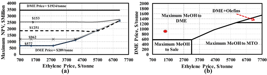
Figure 5. Effect of olefins and DME prices on (a) the maximum NPV of process, (b) optimal product portfolio (Fayetteville shale gas). The base case prices are marked with a red circle.

4. Conclusions

In this study, a techno-economic analysis of a novel polygeneration process for the co-production of DME, olefins, electricity, and methanol using different qualities of shale gas and also conventional natural gas was performed. The impact of power generation alternatives, gas composition and product portfolio on the thermal efficiency of the plant had been presented in part I of this work.

The economic optimization results, presented in this paper, showed that the CLC technology with nickel oxide was the most profitable choice compared to the other power generation options. The results of the sensitivity analysis showed that in most market conditions, it was usually optimal for only one of methanol, DME, or olefins to be co-generated along with electricity. However, the co-production of DME and olefins was optimal for some cases with very high product prices. At current (base case) market conditions, olefin production was not favored. However, using the polygeneration concept, it is possible to produce a mixture of olefins and electricity with 100% CO₂ capture in current market conditions at costs similar to naphtha or ethane cracking without any CO₂ capture. Thus, the proposed process may be a promising way of displacing traditional olefin production using abundant natural gas sources at similar costs but with significantly reduced environmental impact.

Despite promising results achieved by this proposed polygeneration model, the flexibility and dynamic behaviour of this tightly integrated system has not been investigated and is subject of further research. It has been shown previously that flexible polygeneration systems can have massive improvements in NPV compared to inflexible ones. For example, one study showed that up to 62% increases in net present value were possible if the amount of methanol, synthetic fuels, or electricity produced by that particular example process were allowed to change twice per day in response to changes in market prices with a 100% turndown ratio [30]. Other studies on polygeneration systems have shown that the optimal process design and corresponding product portfolio for inflexible polygeneration plants vary significantly with market prices [7]. These studies also showed that the historical variation in market prices experienced over a several year period is sufficiently large enough such that flexible polygeneration may make economic sense. However, all of these studies assumed that transitions between operating steady states were feasible, instantaneous, and free. It is a significant future challenge to construct dynamic models of all of the relevant process units in sufficient detail such that the complex interaction between tightly integrated process sections can be understood well enough such that information about the time required for transitions, feasible turndown ratios, off-spec products, and their associated costs can be known. Some progress has been made in constructing dynamic models of certain individual process units specifically for the purposes of flexible polygeneration applications, such as for gasification [31], steam reforming [32], water gas shift [33], CO₂ capture [34], and solid oxide fuel cells [35]. However, combining these models into one system requires considerable effort and has not yet been achieved.

References

- Xiang, D.; Yang, S.; Li, X.; Qian, Y. Life cycle assessment of energy consumption and GHG emissions of olefins production from alternative resources in China. Energy Convers. Manag. 2015, 90, 12–20. [Google Scholar] [CrossRef]
- Bok, J.-K.; Lee, H.; Park, S. Robust investment model for long-range capacity expansion of chemical processing networks under uncertain demand forecast scenarios. Comput. Chem. Eng. 1998, 22, 1037–1049. [Google Scholar] [CrossRef]
- Ren, T.; Patel, M.K.; Blok, K. Steam cracking and methane to olefins: Energy use, CO2 emissions and production costs. Energy 2008, 33, 817–833. [Google Scholar]
- Gao, L.; Li, H.; Chen, B.; Jin, H.; Lin, R.; Hong, H. Proposal of a natural gas-based polygeneration system for power and methanol production. Energy 2008, 33, 206–212. [Google Scholar] [CrossRef]
- Zhang, X.; Gundersen, T.; Roussanaly, S.; Brunsvold, A.L.; Zhang, S. Carbon chain analysis on a coal IGCC—CCS system with flexible multi-products. Fuel Process. Technol. 2012, 108, 146–153. [Google Scholar] [CrossRef]
- Floudas, C.A.; Elia, J.A.; Baliban, R.C. Hybrid and single feedstock energy processes for liquid transportation fuels: A critical review. Comput. Chem. Eng. 2012, 41, 24–51. [Google Scholar] [CrossRef]
- Adams, T.A., II; Barton, P.I. Combining coal gasification and natural gas reforming for efficient polygeneration. Fuel Process. Technol. 2011, 92, 639–655. [Google Scholar] [CrossRef]
- Adams, T.A., II; Barton, P.I. Combining coal gasification, natural gas reforming, and solid oxide fuel cells for efficient polygeneration with CO2 capture and sequestration. Fuel Process. Technol. 2011, 92, 2105–2115. [Google Scholar] [CrossRef]
- Cormos, C.-C. Assessment of flexible energy vectors poly-generation based on coal and biomass/solid wastes co-gasification with carbon capture. Int. J. Hydrogen Energy 2013, 38, 7855–7866. [Google Scholar] [CrossRef]
- Man, Y.; Yang, S.; Zhang, J.; Qian, Y. Conceptual design of coke-oven gas assisted coal to olefins process for high energy efficiency and low CO2 emission. Appl. Energ. 2014, 133, 197–205. [Google Scholar] [CrossRef]
- Haslbeck, J.L.; Kuehn, N.J.; Lewis, E.G.; Pinkerton, L.L.; Simpson, J.; Turner, M.J.; Varghese, E.; Woods, M.C. Cost and Performance Baseline for Fossil Energy Plants; Volume 1: Bituminous Coal and Natural Gas to Electricity; Department of Energy: Pittsburgh, PA, USA, 2010. [Google Scholar]
- Henry Hub Spot, Average Wholesale Price. Available online: http://www.eia.gov/electricity/wholesale/ (accessed on 1 August 2014).
- Nickel Monoxide, CAS No.: 1313–99–1. Available online: http://www.alibaba.com/product-gs/747545915/Factory_direct_sales_with_reasonable_price.html (accessed on 1 August 2014).
- Adanez, J.; Abad, A.; Garcia-Labiano, F.; Gayan, P.; de Diego, L.F. Progress in chemical-looping combustion and reforming technologies. Prog. Energy Combust. Sci. 2012, 38, 215–282. [Google Scholar] [CrossRef]
- Factory price of Iron Oxide (Fe2O3), CAS No.: 1309–37–1. Available online: http://www.alibaba.com/product-detail/factory-price-of-iron-oxide-fe2o3-_814503142.html?s=p (accessed on 1 August 2014).
- Fan, L.S. Chemical Looping Systems For Fossil Energy Conversions; John Wiley & Sons, Inc.: Hoboken, NJ, USA, 2010. [Google Scholar]
- Electricity Wholesale Price, Average 2014. Available online: http://www.eia.gov/electricity/wholesale/ (acessed on 10 November 2014).
- Methanol Price, North America. October 2014. Available online: https://www.methanex.com/our-business/pricing (accessed on 26 October 2014).
- DiMethyl Ether. Available online: http://www.alibaba.com/product-detail/DiMethyl-Ether_1659793013.html (accessed on 1 June 2014).
- Platts Global Propylene Price Index. August 2014. Available online: http://www.platts.com/news-feature/2014/petrochemicals/pgpi/propylene (accessed on 1 November 2014).
- Platts Global Ethylene Price Index. August 2014. Available online: http://www.platts.com/news-feature/2014/petrochemicals/pgpi/ethylene (accessed on 1 November 2014).
- Peters, M.S.; Timmerhaus, K.D. Plant Design and Economics for Chemical Engineers, 4th ed.; McGraw-Hill: New York, NY, USA, 1991. [Google Scholar]
- CEPCI. Chemical engineering plant cost index. Chem. Eng. 2014, 121, 80. [Google Scholar]
- Parsopoulos, K.E.; Vrahatis, M.N. Particle Swarm Optimization and Intelligence: Advances and Applications; IGI Global: Hershey, PA, USA, 2010. [Google Scholar]
- Gen, M.; Cheng, R. Genetic Algorithms and Engineering Optimization; John Wiley & Sons: New York, NY, USA, 2000. [Google Scholar]
- Goldberg, D.E. Genetic Algorithms in Search, Optimization, and Machine Learning; Addison-Wesley: Boston, MA, USA, 1989. [Google Scholar]
- Diwekar, U.M. Introduction to Applied Optimization; Springer: New York, NY, USA, 2008. [Google Scholar]
- Bertsimas, D.; Tsitsiklis, J. Simulated annealing. Stat. Sci. 1993, 8, 10–15. [Google Scholar] [CrossRef]
- Roberts, T. Ethylene–Good Today, Better Tomorrow–A Year Later. Available online: http://www.lyondellbasell.com/NR/rdonlyres/92CE3892-B543-46FB-9660-00E9AAE8889D/0/GoldmanSachsChemicalIntensity_March27.pdf (accessed on 1 November 2014).
- Chen, Y.; Adams, T.A., II; Barton, P.I. Optimal design and operation of flexible energy polygeneration systems. Ind. Eng. Chem. Res. 2011, 50, 4553–4566. [Google Scholar] [CrossRef]
- Kasule, J.S.; Turton, R.; Bhattacharyya, D.; Zitney, S.E. One-dimensional dynamic modeling of a single-stage downward-firing entrained-flow coal gasifier. Energy Fuels 2014, 28, 4949–4957. [Google Scholar] [CrossRef]
- Ghouse, J.H.; Adams, T.A., II. A multi-scale dynamic two-dimensional heterogeneous model for catalytic steam methane reforming reactors. Int. J. Hydrogen Energy 2013, 38, 9984–9999. [Google Scholar] [CrossRef]
- Adams, T.A., II; Barton, P.I. A dynamic two-dimensional heterogeneous model for water gas shift reactors. Int. J. Hydrogen Energy 2009, 34, 8877–8891. [Google Scholar] [CrossRef]
- Harun, N.; Nittaya, T.; Douglas, P.L.; Croiset, E.; Ricardez-Sandoval, L.A. Dynamic simulation of MEA absorption process for CO2 capture from power plants. Int. J. Greenh. Gas Control 2012, 10, 295–309. [Google Scholar] [CrossRef]
- Harun, N.F.; Tucker, D.; Adams, T.A., II. Fuel composition transients in fuel cell turbine hybrid for polygeneration applications. J. Fuel Cell Sci. Technol. 2014, 11. [Google Scholar] [CrossRef]
© 2015 by the authors; licensee MDPI, Basel, Switzerland. This article is an open access article distributed under the terms and conditions of the Creative Commons Attribution license (http://creativecommons.org/licenses/by/4.0/).